Scalable Bayesian Preference Learning for Crowds

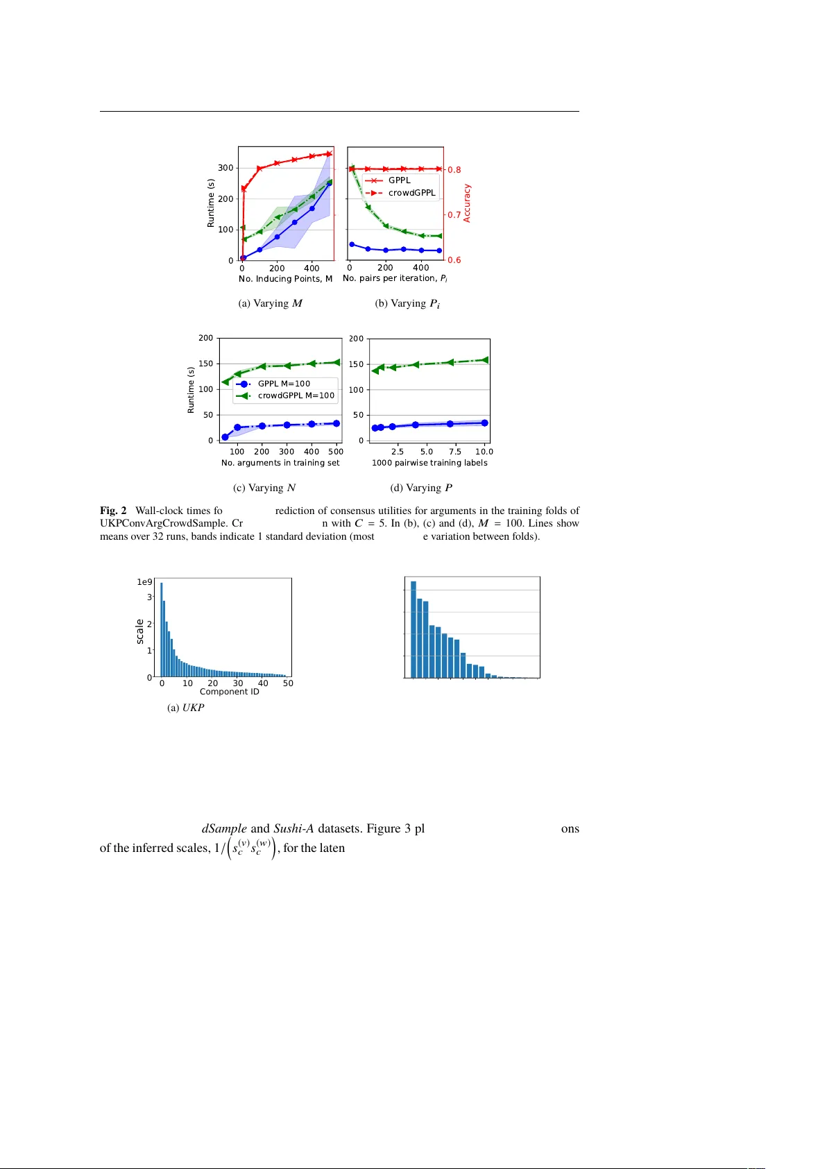
Scalable Ba y esian Pref erence Learning f or Cro wds Edwin Simpson · Iryna Gure vyc h Receiv ed: date Abstract W e propose a scalable Bay esian pref erence lear ning method for jointl y predicting the preferences of individuals as well as the consensus of a cro wd from pair wise labels. Peoples ’ opinions often diﬀer g reatly , making it diﬃcult to predict their pref erences from small amounts of personal data. Individual biases also make it harder to infer the consensus of a cro wd when there are f ew labels per item. W e address these challenges by combining matrix factorisation with Gaussian processes, using a Bay esian approach to account f or uncertainty arising from noisy and sparse data. Our method e xploits input features, such as te xt embeddings and user metadata, to predict pref erences for new items and users that are not in the training set. As previous solutions based on Gaussian processes do not scale to large numbers of users, items or pairwise labels, we propose a stochas tic v ar iational inf erence approach that limits computational and memor y costs. Our experiments on a recommendation task sho w that our method is competitive with pre vious approaches despite our scalable inference approximation. W e demonstrate the method’ s scalability on a natural language processing task with thousands of users and items, and show improv ements ov er the state of the ar t on this task. W e make our software publicly av ailable for future work 1 . 1 Introduction Pr ef erence lear ning in v ol v es compar ing a set of alter natives according to a par ticular qual- ity (Fürnkranz and Hüller meier 2010), which often leads to a div erg ence of opinion betw een people. For e xample, in argument mining, a sub-ﬁeld of natural language processing (NLP), one goal is to rank arguments b y their convincingness (Habernal and Gurevy ch 2016). Whether a par ticular argument is convincing or not depends on the reader’ s point of vie w and prior kno wledg e (Lukin et al. 2017). Similarl y , personal pref erences aﬀect recommender sys tems, which often per f orm better if the y tailor recommendations to a speciﬁc user (Resnic k and V arian 1997). Disagreements also occur when preference annotations are acquired from multiple annotators, f or ex ample, using cro wdsourcing, and are often mitigated b y redundant Edwin Simpson · Iryna Gurevy ch Ubiquitous Know ledge Processing Lab, Dept. of Computer Science, T echnisc he Univ ersität Dar mstadt. E-mail: {simpson,gurevy ch}@ukp.inf or matik.tu-darmstadt.de 1 https://github.com/UKPLab/tacl2018- preference- convincing/tree/crowdGPPL 2 Simpson, E and Gurevy ch, I labelling (Sno w et al. 2008; Banerji et al. 2010). Therefore, we require pref erence learning methods that can account f or diﬀerences of opinion to (1) predict personal pref erences for members of a crowd and (2) infer a consensus given obser vations from multiple users. For both tasks, our goal is to rank items or choose the preferred item from an y giv en pair . Recommender sy stems often predict a user’ s preferences via collaborativ e ﬁltering , which o v ercomes data sparsity by e xploiting similar ities betw een the preferences of diﬀerent users (Resnic k and V arian 1997; Koren et al. 2009). Man y recommender sys tems are based on matrix factorisation techniques that are trained using observations of numer ical ratings. Ho w ev er , diﬀerent annotators often disag ree o v er numer ical annotations and can label incon- sistentl y ov er time (Ovadia 2004; Y annakakis and Hallam 2011), as annotators ma y inter pret the values diﬀerently : a score of 4/5, say , from one annotator may be equivalent to 3/5 from another . The problem is av oided by pair wise labelling , in which the annotator selects their pref erred item from a pair, which can be quick er (Kendall 1948; Kingsley and Bro wn 2010; Y ang and Chen 2011), more accurate (Kiritchenk o and Mohammad 2017), and f acilitates the total sorting of items, as it av oids two items having the same value. Pairwise labels pro vided by a cro wd or extracted from user logs (Joachims 2002) are often noisy and sparse, i.e., many items or users hav e fe w or no labels. This motivates a Ba y esian treatment, which has been sho wn to beneﬁt matr ix factorisation (Salakhutdino v and Mnih 2008) and pref erence lear ning (Chen et al. 2013). Some previous Bay esian methods f or pref erence learning use Gaussian processes (GPs) to account f or input featur es of items or users (Chu and Ghahramani 2005; Houlsby et al. 2012; Khan et al. 2014). These are f eatures that can be e xtracted from content or metadata, such as embeddings (Mikolo v et al. 2013; Dev lin et al. 2019), which are commonly used by NLP methods to represent w ords or documents using a numerical v ector . Input features allo w the model to extrapolate to ne w items or users and mitigate labelling er rors (Felt et al. 2016). How ev er , previous Bay esian pref erence learning methods that account f or input features using GPs do not scale to larg e numbers of items, users, or pairwise labels, as their computational and memory requirements grow with the size of the dataset. In this paper , we propose a scalable Bay esian approach to pair wise preference lear ning with larg e numbers of users or annotators. Our method, crowdGPPL , jointly models personal pref erences and the consensus of a crowd through a combination of matr ix factorisation and Gaussian processes. W e propose a stoc hastic variational infer ence (SVI) scheme (Hoﬀman et al. 2013) that scales to e xtremely larg e datasets, as its memor y complexity and the time comple xity of each iteration are ﬁx ed independently of the size of the dataset. Our ne w approach opens the door to nov el applications inv olving very larg e numbers of users, items and pairwise labels, that would previousl y hav e e x ceeded computational or memory resources and were diﬃcult to parallelise. W e evaluate the method empir ically on tw o real- w orld datasets to demonstrate the scalability of our approach, and its ability to predict both personal pref erences and a consensus giv en pref erences from thousands of users. Our results impro v e per f ormance ov er the previous state-of-the-art (Simpson and Gure vy ch 2018) on a cro wdsourced argumentation dataset, and sho w that modelling personal preferences impro v es predictions of the consensus, and vice v ersa. 2 Related W ork T o obtain a ranking from pairwise labels, many pref erence learning methods model the user’ s choices as a random function of the latent utility of the items. Inf err ing the utilities of items allow s us to rank them, estimate numer ical ratings and predict pair wise labels. Many Scalable Bay esian Preference Learning 3 popular instances of this approach, kno wn as a random utility model (Thurstone 1927), are variants of the Bradley - T er r y (BT) model (Bradley and T er r y 1952; Plac kett 1975; Luce 1959), which assumes a logistic likelihood, or the Thurstone-Mosteller model (Thurstone 1927; Mosteller 1951), which assumes a probit likelihood. R ecent work on the BT model has dev eloped computationall y eﬃcient activ e lear ning, but does not consider input features (Li et al. 2018). Another commonly -used ranking method, SVM-rank (Joachims 2002), predicts pairwise labels from input features without a random utility model, so cannot predict utilities. Gaussian process pref erence learning (GPPL) provides a Bay esian treatment of the random utility model, using input features to predict the utilities of test items and share inf ormation betw een similar items (Chu and Ghahramani 2005). As GPPL can only predict the pref erences of a single user , we introduce a new , scalable approach to model individuals in a crowd. Previous w ork on preference lear ning from cro wdsourced data treats disag reements as annotation er rors and inf ers only the consensus, rather than modelling personal preferences. For instance, Chen et al. (2013) and W ang et al. (2016) tac kle annotator disagreement using Ba y esian approaches that lear n the labelling accuracy of each work er . Recentl y , Pan et al. (2018) and Han et al. (2018) introduced scalable methods that extend this idea from pairwise labels to noisy k -ar y preferences, i.e., totally -ordered subsets of k items. Fu et al. (2016) improv ed SVM-rank by identifying outliers in cro wdsourced data that cor respond to probable er rors, while Uchida et al. (2017) extend SVM-rank to account f or diﬀerent lev els of conﬁdence in each pair wise annotation e xpressed b y the annotators. How ev er , while these approaches diﬀerentiate the lev el of noise f or each annotator, they ignore labelling bias as the diﬀerences between users are not random but depend on personal pref erences tow ard particular items. With small numbers of labels per item, these biases ma y reduce the accuracy of the estimated consensus. Fur thermore, previous aggregation methods for crowdsourced pref erences do not consider item f eatures, so cannot predict the utility of test items (Chen et al. 2013; W ang et al. 2016; Han et al. 2018; Pan et al. 2018; Li et al. 2018). Our approach goes be y ond these methods by predicting personal preferences and incor porating input features. A number of methods use matrix fact orisation to predict personal pref erences from pairwise labels, including Yi et al. (2013), who focus on small numbers of pairs per user, and Salimans et al. (2012), who apply Bay esian matr ix factorisation to handle sparse data. Matrix factorisation represents observed ratings in a user -item matr ix, which it decomposes into two matr ices of low er rank than the user -item matr ix, one corresponding to users and one to items. Users with similar ratings hav e similar columns in the user matr ix, where each entry is a weight ov er a latent rating. By multiplying the low -dimensional representations, w e can predict ratings f or unseen user -item pairs. Kim et al. (2014) use a simpliﬁcation that assumes that each user’ s preferences depend on only one latent ranking. How ev er , previous w orks combining matrix factorisation with pairwise pref erence labels do not account f or input features. This contrasts with work on matrix factorisation with side information, where the ratings or pref erences as well as input features are directly observed, including recent neural netw ork approaches (V olk o vs et al. 2017), Ba y esian approaches that concatenate input f eature vectors with the low -dimensional factored representations (Porteous et al. 2010), and GP -based methods (Adams et al. 2010). Besides pro viding a Bay esian method for matr ix factorisation with both input features and pair wise labels, this paper introduces a much more scalable inf erence method f or a GP-based model. GPs were previousl y used for personal pref erence prediction b y Guo et al. (2010), who propose a GP ov er the joint f eature space of users and items. Since this scales cubically in the number of users, Abbasnejad et al. (2013) propose to cluster users into behavioural groups, but distinct clusters do not allo w for collaborativ e learning betw een users whose pref erences only partially o v erlap, e.g. when tw o users both lik e one genre of music, but 4 Simpson, E and Gurevy ch, I ha v e diﬀerent preferences ov er other genres. Khan et al. (2014) instead lear n a GP for each user , then add a matr ix factorisation ter m that per f or ms collaborative ﬁltering. How ev er, this approach does not model the relationship betw een input features and the lo w-rank matrices, unlike La wrence and U r tasun (2009) who place GP priors o v er latent ratings. Neither of these last tw o methods are full y Bay esian as the users’ weights are optimised rather than marginalised. An alter native is the collaborativ e GP (collabGP) (Houlsb y et al. 2012), which places GP pr iors o v er user weights and latent factors, thereby exploiting input features for both users and items. Ho we v er , unlike our approach, collabGP predicts only pair wise labels, not the utilities of items, which are useful f or rating and ranking, and can only be trained using pair wise labels, ev en if observations of the utilities are av ailable. Fur ther more, exis ting GP -based approaches suﬀer from scalability issues and none of the pre vious methods jointly model the consensus as w ell as personal pref erences in a fully -Bay esian manner . Established methods for GP inference with non-Gaussian likelihoods, such as the Laplace appro ximation and expectation propagation (Rasmussen and Williams 2006), hav e time com- ple xity O ( N 3 ) with N data points and memor y comple xity O ( N 2 ) . For collabGP , Houlsby et al. (2012) use a sparse g eneralized fully independent training conditional (GFITC) ap- pro ximation (Snelson and Ghahramani 2006) to reduce time complexity to O ( P M 2 + U M 2 ) and memor y comple xity to O ( P M + U M ) , where P is the number of pair wise labels, M  P is a ﬁxed number of inducing points, and U is the number of users. How ev er , this is not suﬃciently scalable for very large numbers of users or pairs, due to increasing memory con- sumption and optimisation steps that cannot be distributed. Recent w ork on distributing and parallelising Bay esian matr ix factorisation is not easily applicable to models that incor porate GPs (Ahn et al. 2015; Saha et al. 2015; V ander Aa et al. 2017; Chen et al. 2018). T o handle lar ge numbers of pairwise labels, Khan et al. (2014) subsample the data rather than lear ning from the complete training set. An alternative is stoc hastic variational inf er ence (SVI) (Hoﬀman et al. 2013), which optimises a posterior approximation using a diﬀerent subsample of training data at each iteration, meaning it learns from all training data ov er multiple iterations while limiting costs per iteration. SVI has been applied to GP regression (Hensman et al. 2013) and classiﬁcation (Hensman et al. 2015), fur ther improving scalability o ver earlier sparse approximations. Nguyen and Bonilla (2014) introduce SVI f or multi-output GPs, where each output is a w eighted combination of latent functions. The y apply their method to capture dependencies between regression tasks, treating the weights f or the latent functions as h yper parameters. In this paper , we introduce a Bay esian treatment of the weights and appl y SVI instead to pref erence learning. An SVI method f or GPPL was previously introduced b y Simpson and Gurevy ch (2018), which we detail in Section 4. How ev er, as GPPL does not consider the individual preferences of users in a crowd, we propose a new model, cro wdGPPL, which jointl y models personal preferences and the cro wd consensus using a combination of Gaussian processes and Ba y esian matrix factorisation. 3 Ba yesian Prefer ence Learning for Cro wds W e assume that a pair of items, a and b , ha v e utilities f ( x a ) and f ( x b ) , which represent their value to a user, and that f : R D 7→ R is a function of item features, where x a and x b are v ectors of length D containing the f eatures of items a and b , respectivel y . If f ( x a ) > f ( x b ) , then a is pref er red to b (wr itten a  b ). The outcome of a compar ison between a and b is a pairwise label, y ( a , b ) . Assuming that pairwise labels ne v er contain er rors, then y ( a , b ) = 1 if a  b and 0 other wise. Giv en kno wledg e of f , we can compute the utilities of items in a test set given their f eatures, and the outcomes of pairwise compar isons. Scalable Bay esian Preference Learning 5 Thurstone (1927) proposed the random utility model, which relaxes the assumption that pairwise labels, y ( a , b ) , are alwa ys consistent with the order ing of f ( x a ) and f ( x b ) . Under the random utility model, the likelihood p ( y ( a , b ) = 1 ) increases as f a − f b increases, i.e., as the utility of item a increases relative to the utility of item b . This reﬂects the greater consistency in a user’ s choices when their pref erences are strong er , while accommodating labelling er rors or variations in a user’ s choices o v er time. In the Thurstone-Mosteller model, noise in the observations is explained by a Gaussian-distributed noise ter m, δ ∼ N ( 0 , σ 2 ) : p ( y ( a , b ) | f ( x a ) + δ a , f ( x b ) + δ b ) =  1 if f ( x a ) + δ a ≥ f ( b ) + δ b 0 otherwise, (1) Integrating out the unknown values of δ a and δ b giv es: p ( y ( a , b ) | f ( x a ) , f ( x b )) (2) =  p ( y ( a , b ) | f ( x a ) + δ a , f ( x b ) + δ b )N  δ a ; 0 , σ 2  N  δ b ; 0 , σ 2  d δ a d δ b = Φ ( z ) , where z = f ( x a )− f ( x b ) √ 2 σ 2 , and Φ is the cumulative distribution function of the standard nor mal distribution, meaning that Φ ( z ) is a probit likelihood. 2 This likelihood is also used by Chu and Ghahramani (2005) f or Gaussian process preference lear ning (GPPL), but here we simplify the formulation b y assuming that σ 2 = 0 . 5 , which leads to z having a denominator of √ 2 × 0 . 5 = 1 , hence z = f ( x a ) − f ( x b ) . Instead, we model varying degrees of noise in the pairwise labels by scaling f itself, as we descr ibe in the ne xt section. In practice, f ( x a ) and f ( x b ) must be inf er red from pairwise training labels, y , to obtain a posterior distribution ov er their values. If this posterior is a multiv ariate Gaussian distribution, then the probit lik elihood allow s us to analyticall y marginalise f ( x a ) and f ( x b ) to obtain the probability of a pairwise label: p ( y ( a , b ) | y ) = Φ ( ˆ z ) , ˆ z = ˆ f a − ˆ f b  1 + C a , a + C b , b − 2 C a , b , (3) where ˆ f a and ˆ f b are the means and C is the posterior co variance matr ix of the multivariate Gaussian ov er f ( x a ) and f ( x b ) . Unlik e other choices f or the lik elihood, such as a sigmoid, the probit allo ws us to compute the posterior o v er a pair wise label without fur ther appro ximation, hence we assume this pairwise label likelihood f or our proposed preference learning model. 3.1 GPPL f or Single User Pref erence Learning W e can model the pref erences of a single user by assuming a Gaussian process pr ior o v er the user’ s utility function, f ∼ G P ( 0 , k θ / s ) , where k θ is a kernel function with hyperparameters θ and s is an in v erse scale parameter . The kernel function takes numerical item f eatures as inputs and deter mines the cov ar iance between values of f f or diﬀerent items. The choice of kernel function and its hyperparameters controls the shape and smoothness of the function across the feature space and is often treated as a model selection problem. Kernel functions suitable for a wide range of tasks include the squar ed exponential and the Matérn (Rasmussen and Williams 2006), which both make minimal assumptions but assign higher co variance to 2 Please note that a full list of symbols is pro vided for reference in Appendix E 6 Simpson, E and Gurevy ch, I items with similar f eature values. W e use k θ to compute a co variance matrix K θ , betw een a set of N observed items with features X = { x 1 , . . . , x N } . Here w e e xtend the or iginal deﬁnition of GPPL (Chu and Ghahramani 2005), by intro- ducing the inv erse scale, s , which is drawn from a gamma pr ior , s ∼ G ( α 0 , β 0 ) , with shape α 0 and scale β 0 . The value of 1 / s determines the variance of f , and therefore the magnitude of diﬀerences between f ( x a ) and f ( x b ) f or items a and b . This in tur n aﬀects the lev el of certainty in the pair wise label likelihood as per Equation 2. Giv en a set of P pair wise labels, y = { y 1 , . . . , y P } , where y p = y ( a p , b p ) is the preference label f or items a p and b p , w e can write the joint distr ibution o ver all variables as follo ws: p ( y , f , s | k θ , X , α 0 , β 0 ) = P  p = 1 p ( y p | f )N ( f ; 0 , K θ / s ) G ( s ; α 0 , β 0 ) (4) where f = { f ( x 1 ) , . . . , f ( x N )} is a v ector containing the utilities of the N items ref er red to b y y , and p ( y p | f ) = Φ  z p  is the pairwise likelihood (Equation 2). 3.2 Crowd Pref erence Learning T o predict the pref erences of individuals in a crowd, we could use an independent GPPL model f or each user . Ho we v er , b y modelling all users jointl y , we can e xploit correlations betw een their interests to impro v e predictions when preference data is sparse, and reduce the memor y cost of s toring separate models. Cor relations betw een users can ar ise from common interests o ver cer tain subsets of items, such as in one par ticular g enre in a book recommendation task. Identifying such cor relations helps to predict pref erences from fe wer observations and is the core idea of collaborative ﬁlter ing (R esnick and V ar ian 1997) and matrix factorisation (Koren et al. 2009). As well as individual preferences, we wish to predict the consensus by aggregating pref- erence labels from multiple users. Individual biases of diﬀerent users may aﬀect consensus predictions, particularly when data f or cer tain items comes from a small subset of users. The consensus could also help predict pref erences of users with little or no data by fa v our ing popular items and av oiding generall y poor items. W e therefore propose crowdGPPL , which jointly models the preferences of individual users as well as the underl ying consensus of the cro wd. Unlik e previous methods for inferr ing the consensus, such as Cro wdBT (Chen et al. 2013), we do not treat diﬀerences betw een users as simply the result of labelling er rors, but also account f or their subjective biases tow ards par ticular items. For crowdGPPL, we represent utilities in a matr ix, F ∈ R N × U , with U columns corre- sponding to users. Within F , each entr y F a , j = f ( x a , u j ) is the utility f or item a f or user j with user f eatures u j . W e assume that F = V T W + t 1 T is the product of two low -rank matrices plus a column vector of consensus utilities, t ∈ R N , where W ∈ R C × U is a latent representation of the users, V ∈ R C × N is a latent representation of the items, C is the number of latent components , i.e., the dimension of the latent representations, and 1 is a column v ector of ones of length U . The column v . , a of V , and the column w . , j of W , are latent v ector representations of item a and user j , respectivel y . Each ro w of V , v c = { v c ( x 1 ) , . . . , v c ( x N )} , contains ev aluations of a latent function, v c ∼ G P ( 0 , k θ / s ( v ) c ) , of item features, x a , where k is a kernel function, s ( v ) c is an inv erse function scale, and θ are kernel h yperparameters. The consensus utilities, t = { t ( x 1 ) , . . . , t ( x N )} , are values of a consensus utility function o v er item f eatures, t ∼ G P ( 0 , k θ / s ( t ) ) , which is shared across all users, with in verse scale s ( t ) . Similarl y , each ro w of W , w c = { w c ( u 1 ) , . . . , w c ( u U )} , contains evaluations of a latent Scalable Bay esian Preference Learning 7 function, w c ∼ G P ( 0 , k η / s ( w ) c ) , of user f eatures, u j , with inv erse scale s ( w ) c and kernel hy - perparameters η . Therefore, eac h utility in F can be wr itten as a weighted sum ov er the latent components: f ( x a , u j ) = C  c = 1 v c ( x a ) w c ( u j ) + t ( x a ) , (5) where u j are the features of user j and x a are the features of item a . Each latent component corresponds to a utility function f or certain items, which is shared by a subset of users to diﬀering deg rees. For ex ample, in the case of book recommendation, c could relate to science ﬁction no v els, v c to a ranking ov er them, and w c to the degree of agreement of users with that ranking. The individual preferences of each user j deviate from a consensus across users, t , according to  C c = 1 v c ( x a ) w c ( u j ) . This allow s us to subtract the eﬀect of individual biases when inferr ing the consensus utilities. The consensus can also help when inf err ing personal pref erences for new combinations of users and items that are very diﬀerent to those in the training data b y accounting f or any objective or widespread appeal that an item may hav e. Although the model assumes a ﬁx ed number of components, C , the GP priors o ver w c and v c act as shrink ag e or ARD priors that fa v our values close to zero (MacKa y 1995; Psorakis et al. 2011). Components that are not required to e xplain the data will hav e poster ior e xpectations and scales 1 / s ( v ) and 1 / s ( w ) approaching zero. Theref ore, it is not necessar y to optimise the value of C by hand, pro viding a suﬃciently larg e number is chosen. Equation 5 is similar to cross-task crowdsour cing (Mo et al. 2013), which uses matr ix factorisation to model annotator per f ormance in diﬀerent tasks, where t corresponds to the objectiv e diﬃculty of a task. Ho we ver , unlik e cro wdGPPL, the y do not use GPs to model the factors, nor appl y the approach to pref erence learning. For preference lear ning, collabGP (Houlsb y et al. 2012) is a related model that e xcludes the consensus and uses values in v c to represent pairs rather than individual items, so does not infer item ratings. It also omits scale parameters for the GPs that encourage shrinkage when C is larg er than required. W e combine the matrix factorisation method with the preference likelihood of Equation 2 to obtain the joint pref erence model f or multiple users, crowdGPPL : p  y , V , W , t , s ( v ) 1 , . . , s ( v ) C , s ( w ) 1 , . . , s ( w ) C , s ( t ) | k θ , X , k η , U , α ( t ) 0 , β ( t ) 0 , α ( v ) 0 , β ( v ) 0 , α ( w ) 0 , β ( w ) 0  = P  p = 1 Φ  z p  N  t ; 0 , K θ / s ( t )  G  s ( t ) ; α ( t ) 0 , β ( t ) 0  C  c = 1  N  v c ; 0 , K θ / s ( v ) c  N  w c ; 0 , L η / s ( w ) c  G  s ( v ) c ; α ( v ) 0 , β ( v ) 0  G  s ( w ) c ; α ( w ) 0 , β ( w ) 0   , (6) where z p = v T . , a p w . , u p + t a p − v T . , b p w . , u p − t b p , index p refers to a user and a pair of items, { u p , a p , b p } , U is the set of feature v ectors for all users, K θ is the prior cov ar iance for the items as in GPPL, and L η is the prior cov ar iance f or the users computed using k η . 4 Scalable Infer ence Giv en a set of pairwise training labels, y , w e aim to ﬁnd the poster ior ov er the matr ix F ∗ = V ∗ T W ∗ of utilities for test items and tes t users, and the pos terior o ver consensus utilities f or test items, t ∗ . The non-Gaussian likelihood (Equation 2) makes ex act inf erence 8 Simpson, E and Gurevy ch, I intractable, hence previous w ork uses the Laplace appro ximation f or GPPL (Chu and Ghahra- mani 2005) or combines expectation propagation (EP) with v ariational Bay es f or a multi-user model (Houlsby et al. 2012). The Laplace appro ximation is a maximum a-posterior i solution that takes the most probable v alues of parameters rather than integrating o ver their distri- butions, and has been sho wn to per f orm poorl y f or classiﬁcation compared to EP (Nickisch and Rasmussen 2008). How ev er, a drawbac k of EP is that con verg ence is not guaranteed (Minka 2001). More impor tantly , inference f or a GP using either method has computational comple xity O ( N 3 ) and memory complexity O ( N 2 ) , where N is the number of data points. The cost of inference can be reduced using a sparse approximation based on a set of inducing points , which act as substitutes f or the points in the training dataset. By choosing a ﬁx ed number of inducing points, M  N , the computational cost is cut to O ( N M 2 ) , and the memory comple xity to O ( N M ) . Inducing points must be selected using either heuristics or by optimising their positions to maximise an estimate of the marginal lik elihood. One such sparse appro ximation is the g eneralized fully independent training conditional (GFITC) (Naish- guzman and Holden 2008; Snelson and Ghahramani 2006), used b y Houlsb y et al. (2012) f or collabGP . How ev er , time and memor y costs that g ro w linearly with O ( N ) star t to become a problem with thousands of data points, as all data must be processed in ev er y iterative update, bef ore any other parameters such as s are updated, making GFITC unsuitable f or v ery large datasets (Hensman et al. 2015). W e derive a more scalable approach f or GPPL and cro wdGPPL using stochas tic varia- tional inference (SVI) (Hoﬀman et al. 2013). For GPPL, this reduces the time complexity of each iteration to O ( P i M 2 + P 2 i M + M 3 ) , and memor y comple xity to O ( P i M + M 2 + P 2 i ) , where P i is a mini-batch size that we choose in advance. Neither P i nor M are dependent on the size of the dataset, meaning that SVI can be run with arbitrar ily larg e datasets, and other model parameters such as s can be updated bef ore processing all data to encourage fas ter con v erg ence. First, we deﬁne a suitable likelihood appro ximation to enable the use of S VI. 4.1 Approximating the Pos ter ior with a Pairwise Likelihood The pref erence likelihood in Equation 2 is not conjugate with the Gaussian process, which means there is no analytic e xpression f or the e xact posterior . For single-user GPPL, w e theref ore approximate the preference likelihood with a Gaussian: p ( f | y , s ) ∝ P  p = 1 p  y p | z p  p ( f | K , s ) = P  p = 1 Φ  z p  N ( f ; 0 , K / s ) (7) ≈ P  p = 1 N  y p ; Φ ( z p ) , Q p , p  N ( f ; 0 , K / s ) = N ( y ; Φ ( z ) , Q ) N ( f ; 0 , K / s ) , where Q is a diagonal noise co variance matr ix and we omit the kernel hyperparameters, θ , to simplify notation. For cro wdGPPL, we use the same appro ximation to the likelihood, but replace f with F . W e estimate the diagonals of Q b y moment matching our approximate likelihood with Φ ( z p ) , which deﬁnes a Ber noulli distribution with variance Q p , p = Φ ( z p )( 1 − Φ ( z p )) . How ev er , this means that Q depends on z and theref ore on f , so the approximate posterior o v er f cannot be computed in closed form. T o resolv e this, we approximate Q p , p using an estimated poster ior o v er Φ ( z p ) computed independently for each pair wise label, p . W e obtain this estimate by updating the parameters of the conjugate pr ior for the Bernoulli likelihood, which is a beta distribution with parameters γ and λ . W e ﬁnd γ and λ by Scalable Bay esian Preference Learning 9 matching the moments of the beta prior to the pr ior mean and variance of Φ ( z p ) , estimated using numer ical integration. The pr ior ov er Φ ( z p ) is deﬁned b y a GP f or single-user GPPL, p ( Φ ( z p ) | K , α 0 , β 0 ) , and a non-standard distribution f or cro wdGPPL. Giv en the obser v ed label y p , w e estimate the diagonals in Q as the variance of the posterior beta-Ber noulli: Q p , p ≈ ( γ + y p )( λ + 1 − y p ) ( γ + λ + 1 ) 2 . (8) The cov ariance Q theref ore appro ximates the expected noise in the observations, hence captures variance due to σ in Equation 2. This approximation performs well empir ically f or Gaussian process classiﬁcation (Reece et al. 2011; Simpson et al. 2017) and classiﬁcation using e xtended Kalman ﬁlters (Lee and R ober ts 2010; Lowne et al. 2010). U nf or tunately , the nonlinear ter m Φ ( z ) means that the poster ior is still intractable, so we replace Φ ( z ) with a linear function of f by taking the ﬁrst-order T ay lor ser ies e xpansion of Φ ( z ) about the expectation E [ f ] = ˆ f : Φ ( z ) ≈ ˜ Φ ( z ) = G  f − ˆ f  + Φ ( ˆ z ) , (9) G p , i = ∂ Φ ( ˆ z p ) ∂ f i = Φ ( ˆ z p )  1 − Φ ( ˆ z p )   2 y p − 1   [ i = a p ] − [ i = b p ]  , (10) where ˆ z is the expectation of z computed using Equation 3, and [ i = a ] = 1 if i = a and is 0 other wise. There is a circular dependency between ˆ f , which is needed to compute ˆ z , and G . W e estimate these terms using a variational inference procedure that iterates betw een updating f and G (S teinberg and Bonilla 2014) as part of Algorithm 1. The complete appro ximate posterior f or GPPL is now as follo ws: p ( f | y , s ) ≈ N ( y ; G ( f − E [ f ]) + Φ ( ˆ z ) , Q ) N ( f ; 0 , K / s ) / Z = N  f ; ˆ f , C  , (11) where Z is a normalisation constant. Linear isation means that our approximate likelihood is conjugate to the pr ior, so the approximate posterior is also Gaussian. Gaussian approxi- mations to the poster ior hav e sho wn strong empir ical results f or classiﬁcation (Nickisch and Rasmussen 2008) and preference lear ning (Houlsby et al. 2012), and linear isation using a T ay lor expansion has been widely tested in the extended Kalman ﬁlter (Haykin 2001) as w ell as Gaussian processes (Steinber g and Bonilla 2014; Bonilla et al. 2016). 4.2 SVI f or Single User GPPL Using the linear approximation in the previous section, posterior inference requires inv er ting K with computational cost O ( N 3 ) and taking an expectation with respect to s , which remains intractable. W e address these problems using stoc hastic variational inf erence (S VI) with a sparse approximation to the GP that limits the size of the cov ar iance matrices w e need to in v er t. W e introduce M  N inducing items with inputs X m , utilities f m , and co variance K mm . The cov ar iance between the observ ed and inducing items is K nm . For clarity , we omit θ from this point on. W e assume a mean-ﬁeld appro ximation to the joint posterior o v er inducing and training items that factorises between diﬀerent sets of latent variables: p ( f , f m , s | y , X , X m , k θ , α 0 , β 0 ) ≈ q ( f , f m , s ) = q ( s ) q ( f ) q ( f m ) , (12) where q ( . ) are variational factor s deﬁned below . Each factor corresponds to a subset of latent variables, ζ i , and takes the form ln q ( ζ i ) = E j , i [ ln p ( ζ i , x , y )] . That is, the expectation with 10 Simpson, E and Gurevy ch, I respect to all other latent variables, ζ j , ∀ j , i , of the log joint distribution of the obser v ations and latent variables, ζ i . T o obtain the factor f or f m , we marginalise f and take e xpectations with respect to q ( s ) : ln q ( f m ) = ln N  y ; ˜ Φ ( z ) , Q  + ln N  f m ; 0 , K mm E [ s ]  + const = ln N  f m ; ˆ f m , S  , (13) where the variational parameters ˆ f m and S are computed using an iterative SVI procedure described belo w . W e choose an appro ximation of q ( f ) that depends only on the inducing point utilities, f m , and is independent of the observations: ln q ( f ) = ln N  f ; A ˆ f m , K + A ( S − K mm / E [ s ] ) A T  , (14) where A = K nm K − 1 mm . Theref ore, we no longer need to inv er t an N × N cov ar iance matr ix to compute q ( f ) . The factor q ( s ) also depends only the inducing points: ln q ( s ) = E q ( f m ) [ ln N ( f m | 0 , K mm / s )] + ln G ( s ; α 0 , β 0 ) + const = ln G ( s ; α , β ) , (15) where α = α 0 + M 2 and β = β 0 + 1 2 tr  K − 1 mm  S + ˆ f m ˆ f T m   . The e xpected v alue is E [ s ] = α β . W e appl y variational inf erence to iterativ ely reduce the KL -div erg ence between our appro ximate posterior and the tr ue posterior (Equation 12) by maximising a low er bound, L , on the log marginal likelihood (detailed equations in Appendix A), which is given by : ln p ( y | K , α 0 , β 0 ) = KL ( q ( f , f m , s ) | | p ( f , f m , s | y , K , α 0 , β 0 )) + L (16) L = E q ( f ) [ ln p ( y | f ) ] + E q ( f m , s ) [ ln p ( f m , s | K , α 0 , β 0 ) − ln q ( f m ) − ln q ( s ) ] . T o optimise L , we initialise the q factors randomly , then update each one in turn, taking e xpectations with respect to the other f actors. The only term in L that ref ers to the obser vations, y , is a sum of P ter ms, each of which ref ers to one obser vation only . This means that L can be maximised by considering a random subset of observations at each iteration (Hensman et al. 2013). For the i th update of q ( f m ) , w e randomly select P i observations y i = { y p ∀ p ∈ P i } , where P i is a random subset of inde x es of observations, and P i is a mini-batch size. The items ref er red to by the pairs in the subset are N i = { a p ∀ p ∈ P i } ∪ { b p ∀ p ∈ P i } . W e per form updates using Q i (ro w s and columns of Q f or pairs in P i ), K i m and A i (ro w s of K nm and A in N i ), G i (ro w s of G in P i and columns in N i ), and ˆ z i =  ˆ z p ∀ p ∈ P i  . The updates optimise the natural parameters of the Gaussian distribution by f ollowing the natural g radient (Hensman et al. 2015): S − 1 i = ( 1 − ρ i ) S − 1 i − 1 + ρ i  E [ s ] K − 1 mm + π i A T i G T i Q − 1 i G i A i  (17) ˆ f m , i = S i  ( 1 − ρ i ) S − 1 i − 1 ˆ f m , i − 1 + ρ i π i A T i G T i Q − 1 i  y i − Φ ( ˆ z i ) + G i A i ˆ f m , i − 1   (18) where ρ i = ( i +  ) − r is a mixing coeﬃcient that controls the update rate, π i = P P i w eights each update according to sample size,  is a dela y hyperparameter and r is a for getting rate (Hoﬀman et al. 2013). By performing updates in ter ms of mini-batches, the time comple xity of Equations 17 and 18 is O ( P i M 2 + P 2 i M + M 3 ) and memor y complexity is O ( M 2 + P 2 i + M P i ) . The only parameters that must be stored betw een iterations relate to the inducing points, hence the memory consumption does not g ro w with the dataset size as in the GFITC approximation used b y Houlsb y et al. (2012). A further adv antage of stoc hastic updating is that the s Scalable Bay esian Preference Learning 11 parameter (and an y other global parameters not immediately depending on the data) can be learned bef ore the entire dataset has been processed, which means that poor initial estimates of s are rapidly improv ed and the algor ithm can conv erg e faster . Input: P air wise labels, y , training item features, x , test item features x ∗ 1 Select inducing point locations x m m and compute kernel matrices K , K m m and K n m giv en x ; 2 Initialise E [ s ] and ˆ f m to pr ior means and S to prior cov ar iance K m m ; while L not conver g ed do 3 Select random sample, P i , of P obser vations; while G i not conver ged do 4 Compute E [ f i ] ; 5 Compute G i giv en E [ f i ] ; 6 Compute ˆ f m , i and S i ; end 7 Update q ( s ) and compute E [ s ] and E [ ln s ] ; end 8 Compute kernel matrices for test items, K ∗∗ and K ∗ m , given x ∗ ; 9 Use conv erged values of E [ f ] and ˆ f m to estimate poster ior ov er f ∗ at test points ; Output: P osterior mean of the test values, E [ f ∗ ] , and cov ar iance, C ∗ Algorithm 1: The SVI algorithm for GPPL: preference learning with a single user. The complete SVI algorithm is summar ised in Algorithm 1. It uses a nested loop to lear n G i , which a voids storing the complete matr ix, G . It is possible to distribute computation in lines 3-6 by selecting multiple random samples to process in parallel. A global estimate of ˆ f m and S is passed to each compute node, which runs the loop o ver lines 4 to 6. The resulting updated ˆ f m and S values are then passed back to a central node that combines them b y taking a mean w eighted by π i to account f or the size of each batch. Inducing point locations can be learned as par t of the v ariational inf erence procedure, which breaks conv erg ence guarantees, or by an expensiv e optimisation process (Hensman et al. 2015). W e obtain good per f ormance by choosing inducing points up-front using K - means++ (Ar thur and V assilvitskii 2007) with M clusters to cluster the f eature vectors, then taking the cluster centres as inducing points that represent the distribution of obser vations. The inf er red distribution ov er the inducing points can be used to estimate the posteriors of test items, f ( x ∗ ) , according to: f ∗ = K ∗ m K − 1 mm ˆ f m , C ∗ = K ∗∗ + K ∗ m K − 1 mm ( S − K mm / E [ s ]) K − 1 mm K T ∗ m , (19) where C ∗ is the posterior co variance of the test items, K ∗∗ is their prior cov ar iance, and K ∗ m is the co v ar iance between test and inducing items. 4.3 SVI f or Cro wdGPPL W e now provide the variational posterior f or the cro wdGPPL model deﬁned in Equation 6: p  V , V m , W , W m , t , t m , s ( v ) 1 , . . , s ( v ) C , s ( w ) 1 , . . , s ( w ) C , s ( t ) | y , X , X m , U , U m , k , α 0 , β 0  ≈ q ( t ) q ( t m ) q  s ( t )  C  c = 1 q ( v c ) q ( w c ) q ( v c , m ) q ( w c , m ) q  s ( v ) c  q  s ( w ) c  , (20) 12 Simpson, E and Gurevy ch, I where U m are the feature vectors of inducing users and the variational q factors are deﬁned belo w . W e use SVI to optimise the low er bound on the log marginal likelihood (detailed in Appendix B), which is given by : L cr = E q ( F ) [ ln p ( y | F )] + E q ( t m , s ( t ) )  ln p  t m , s ( t ) | K mm , α ( t ) 0 , β ( t ) 0  − ln q ( t m ) − ln q  s ( t )   + C  c = 1  E q  v m , c , s ( v ) c   ln p  v m , c , s ( v ) c | K mm , α ( v ) 0 , β ( v ) 0  − ln q ( v m , c ) − ln q  s ( v ) c   + E q  w m , c , s ( w ) c   ln p  w m , c , s ( w ) c | L mm , α ( w ) 0 , β ( w ) 0  − ln q ( w m , c ) − ln q  s ( w ) c    . (21) The S VI algorithm follo ws the same pattern as Algor ithm 1, updating each q factor in tur n b y computing means and cov ar iances f or V m , W m and t m instead of f m (see Algor ithm 2). The time and memor y comple xity of each update are O ( C M 3 items + C M 2 items P i + C M items P 2 i + C M 3 users + C M 2 users P i + C M users P 2 i ) and O ( C M 2 items + P 2 i + M items P i + C M 2 users + M users P i ) , respectiv el y . The variational factor for the c th inducing item component is: ln q ( v m , c ) = E q ( t , w m , c 0 ∀ c 0 , v m , c 0 ∀ c 0 \ c )  ln N  y ; ˜ Φ ( z ) , Q   + ln N     v m , c ; 0 , K mm E  s ( v ) c      + const = ln N  v m , c ; ˆ v m , c , S ( v ) c  , (22) where posterior mean ˆ v m , c and co variance S ( v ) c are computed using equations of the same f or m as Equations 17 and 18, ex cept Q − 1 is scaled by expectations o v er w m , c , and ˆ f m , i is replaced b y ˆ v m , c , i . The factor f or the inducing points of t f ollow s a similar patter n to v m , c : ln q ( t m ) = E q ( w m , c ∀ c , v m , c ∀ c )  ln N  y ; ˜ Φ ( z ) , Q   + ln N  t m ; 0 , K mm E [ s ( t ) ]  + const = ln N  t m ; ˆ t m , S ( t )  , (23) where the equations f or ˆ t and S ( t ) are the same as Equations 17 and 18, e xcept ˆ f m , i is replaced b y ˆ t m , i . Finall y , the variational distribution for each inducing user’ s component is: ln q ( w m , c ) = E q ( t , w m , c 0 ∀ c 0 \ c , v m , c 0 ∀ c 0 )  ln N  y ; ˜ Φ ( z ) , Q   + ln N  w m , c ; 0 , L mm E [ s ( w ) c ]  + const = ln N  w m , c ; ˆ w m , c , Σ c  , (24) where ˆ w c and Σ c also f ollow the pattern of Equations 17 and 18, with Q − 1 scaled b y e xpectations of w c , m , and ˆ f m , i replaced by ˆ w m , c , i . W e provide the complete equations f or the variational means and cov ar iances f or v m , c , t m and w m , c in Appendix C. The expectations f or inv erse scales, s ( v ) 1 , . . , s ( v ) c , s ( w ) 1 , . . , s ( w ) c and s ( t ) can be computed using Equation 15 by substituting the cor responding ter ms f or v c , w c or t instead of f . Predictions f or cro wdGPPL can be made by computing the posterior mean utilities, F ∗ , and the co v ar iance Λ ∗ u f or each user , u , in the test set: F ∗ = ˆ t ∗ + C  c = 1 ˆ v ∗ T c ˆ w ∗ c , Λ ∗ u = C ∗ t + C  c = 1 ω ∗ c , u C ∗ v , c + ˆ w 2 c , u C ∗ v , c + ω ∗ c , u ˆ v c ˆ v T c , (25) Scalable Bay esian Preference Learning 13 where ˆ t ∗ , ˆ v ∗ c and ˆ w ∗ c are posterior test means, C ∗ t and C ∗ v , c are posterior co variances of the test items, and ω ∗ c , u is the posterior variance of the user components f or u . (see Appendix D, Equations 39 to 41). The mean F ∗ and cov ar iances Λ ∗ u can be inser ted into Equation 2 to predict pair wise labels. In practice, the full cov ar iance ter ms are needed only for Equation 2, so need only be computed betw een items f or which we wish to predict pair wise labels. 5 Experiments Dataset #f olds/ #users total training set test set #f eatures samples #items #pairs #pairs #items items users Simulation a and b 25 25 100 900 0 100 2 2 Simulation c 25 25 100 36–2304 0 100 2 2 Sushi A-small 25 100 10 500 2500 10 18 123 Sushi A 25 100 10 2000 2500 10 18 123 Sushi B 25 5000 100 50000 5000 100 18 123 UKPConvAr gCrowdSample 32 1442 1052 16398 529 33 32310 0 T able 1 Summary of datasets showing av erage counts for the training and test sets used in each fold/subsample. The test sets all contain gold-standard rankings ov er items as well as pair wise labels, ex cept the simulations, which are not generated as we ev aluate using the rankings onl y . Numbers of features are given after categorical labels hav e been conv er ted to one-hot encoding, counting each categor y as a separate feature. Our e xperiments test ke y aspects of crowdGPPL: predicting consensus utilities and personal pref erences from pair wise labels and the scalability of our proposed SVI method. In Section 5.1, w e use simulated data to test the robustness of cro wdGPPL to noise and unkno wn numbers of latent components. Section 5.2 compares diﬀerent conﬁgurations of the model against alter nativ e methods using the Sushi datasets 3 (Kamishima 2003). Section 5.3 ev aluates prediction per f or mance and scalability of cro wdGPPL in a high-dimensional NLP task with sparse, noisy crowdsourced pref erences ( UKPConvArgCr owdSample 4 , Simpson and Gurevy ch (2018)). Finall y , Section 5.4 evaluates whether cro wdGPPL ignores redundant components. The datasets are summarised in T able 1. As baselines, w e compare cro wdGPPL agains t GPPL , which we train on all users’ pref erence labels to lear n a single utility function, and GPPL -per -user , in which a separate GPPL instance is learned f or each user with no collaborative learning. W e also compare agains t the GPVU model (Khan et al. 2014) and collabGP (Houlsb y et al. 2012). CollabGP contains parameters f or each pairwise label and each user , so has a larger memor y f ootprint than our SVI scheme, which stores only the moments at the inducing points. W e test cr owdBT (Chen et al. 2013) as par t of a method for predicting consensus utilities from crowdsourced pairwise preferences. Cro wdBT models each w orker ’s accuracy , assuming that the diﬀerences betw een w orkers ’ labels are due to random er rors rather than subjectiv e preferences. Since cro wdBT does not account for the item features, it cannot predict utilities for items that were not par t of the training set. W e therefore treat the posterior mean utilities produced by crowdBT as training labels f or Gaussian process reg ression using SVI. W e set the obser vation noise variance of the GP equal to the crowdBT posterior 3 http://www.kamishima.net/sushi/ 4 https://github.com/ukplab/tacl2018- preference- convincing 14 Simpson, E and Gurevy ch, I 0.10 0.15 0.20 0.25 noise rate in pairwise training labels 0.3 0.4 0.5 0.6 0.7 ( t e s t s e t ) GPPL-per-user GPPL crowdGPPL (a) Consensus 0.05 0.10 0.15 0.20 0.25 0.30 noise rate in pairwise training labels 0.1 0.2 0.3 0.4 ( t e s t s e t ) GPPL-per-user GPPL crowdGPPL (b) Personal preferences 500 1000 1500 2000 2500 number of pairwise training labels 0.1 0.2 0.3 0.4 0.5 0.6 0.7 Mean factor correlation (Pearson's r) C = 1 C = 3 C = 1 0 C = 2 0 (c) Latent factors Fig. 1 Simulations: rank cor relation between tr ue and inferred utilities. (a) & (b) vary the lev el of noise in pairwise training labels, (c) varies the number of pair wise training labels. variance of the utilities to propag ate uncer tainty from cro wdBT to the GP . This pipeline method, crowdBT –GP , tests whether it is suﬃcient to treat annotator diﬀerences as noise, in contrast to the crowdGPPL approach of modelling individual preferences. W e ev aluate the methods using the f ollo wing metr ics: accuracy (acc) , which is the frac- tion of correct pair wise labels; cross entr opy error (CEE) between the posterior probabilities o v er pairwise labels and the tr ue labels, which captures the quality of the pair wise posterior; and Kendall’ s τ , which ev aluates the ranking obtained b y sor ting items b y predicted utility . 5.1 Simulated Noisy Data Firs t, we ev aluate whether crowdGPPL is able to model individual pref erences with varying amounts of labelling noise. W e set the number of latent components to C = 20 and all Gamma hyperparameters for crowdGPPL, GPPL and GPPL -per -user to α 0 = 1 , β 0 = 100 . W e use Matér n 3/2 kernels with the length-scale for each dimension of the feature v ector , d , chosen by a median heur istic: l d , MH = median ({ | | x i , d − x j , d | | , ∀ i = 1 , . . , N , ∀ j = 1 , . . ., N } ) . (26) This is a computationally fr ugal wa y to choose the length-scales, that has been extensiv ely used in various kernel methods (e.g., Bors and Pitas (1996); Gretton et al. (2012)). The SVI h yper parameters were set to ρ = 0 . 9 , P i = 1000 and  = 1 . Hoﬀman et al. (2013) found that higher values of ρ ga v e better ﬁnal results but slightly slo wer conv ergence, recommending 0 . 9 as a good balance across sev eral datasets, and did not ﬁnd any eﬀect from changing  . W e follo w their recommendations and do not ﬁnd it necessary to per f orm fur ther tuning in our e xperiments. Both M and P i are constrained in practice by the computational resources a vailable – we inv estig ate these further in Section 5.3. In simulation (a), to test consensus prediction, we generate a 20 × 20 gr id of points and split them into 50% training and test sets. For each gr idpoint, w e generate pair wise labels by dra wing from the generativ e model of crowdGPPL with U = 20 users, C = 5 , each s ( v ) c set to random values between 0.1 and 10, and s ( w ) c = 1 , ∀ c . W e vary s ( t ) to control the noise in the consensus function. W e train and test cro wdGPPL with C = U and repeat the complete e xperiment 25 times, including generating new data. Figure 1a show s that cro wdGPPL better recov ers the consensus ranking than the base- lines, ev en as noise increases, as GPPL ’ s predictions are w orsened b y biased users who Scalable Bay esian Preference Learning 15 Sushi-A -small Sushi-A Sushi-B Method Acc CEE τ Acc CEE τ A cc CEE τ cro wdGPPL .71 .56 .48 .84 .33 .79 .76 .50 . 54 cro wdGPPL \ inducing .70 .60 .45 .84 .34 .78 - - - cro wdGPPL \ u .70 .58 .46 .85 .31 .80 .78 .50 .57 cro wdGPPL \ u \ x .71 .57 .49 .85 .33 .80 .77 .49 .56 cro wdGPPL \ u , \ t .68 .60 .43 .84 .33 .80 .76 .51 .58 GPPL .65 .62 .31 .65 .62 .31 .65 .62 .31 GPPL-per-user .67 .64 .42 .83 .40 .79 .75 .60 .60 collabGP .69 .58 n/a .83 .35 n/a .76 .49 n/a collabGP \ u .69 .59 n/a .84 .33 n/a .76 .50 n/a GPVU .70 .67 .43 .72 .67 .42 .73 .59 .52 T able 2 Predicting personal preferences on Sushi datasets, means o v er 25 repeats. The standard deviations are ≤ 0 . 02 f or all accuracies, ≤ 0 . 08 for all CEE, and ≤ 0 . 03 for all τ . For Sushi-B, cro wdGPPL, GPPL -per -user and collabGP had runtimes of 30 minutes on a 12 core, 2.6GHz CPU server; GPPL required only 1 minute. deviate consistentl y from the consensus. For GPPL -per -user, the consensus is simply the mean of all users’ predicted utilities, so does not beneﬁt from shar ing inf ormation between users when training. For simulation (b), we modify the previous setup by ﬁxing s ( t ) = 5 and varying s ( v ) c , ∀ c to ev aluate the methods ’ ability to reco v er the personal pref erences of simu- lated users. The results in Figure 1b show that crowdGPPL is able to make better predictions when noise is belo w 0 . 3 . W e hypothesise that crowdGPPL can recov er latent components giv en suﬃcient train- ing data. In simulation (c), we generate data using the same setup as bef ore, but ﬁx s ( t ) = s ( v ) c = s ( w ) = 1 , ∀ c and vary the number of pairwise training labels and the num- ber of tr ue components through C true ∈ { 1 , 3 , 10 , 20 } . W e match inf erred components to the true components as follo ws: compute Pearson cor relations betw een each unmatched true component and each unmatched inferred component; select the pair with the highest cor re- lation as a match; repeat until all tr ue components are matched. In Figure 1c w e plot the mean cor relation between matched pairs of components. For all values of C true , increasing the number of training labels bey ond 700 br ings little impro v ement. Perf or mance is highest when C true = 20 , possibly because the predictive model has C = 20 , so is a closer match to the generating model. Ho we v er , crowdGPPL is able to recov er latent components reasonably w ell f or all values of C true giv en > 500 labels, despite mismatches between C and C true . 5.2 Sushi Preferences The sushi datasets contain, f or each user , a gold standard pref erence ranking of 10 types of sushi, from which we generate gold-standard pair wise labels. T o test per formance with v ery f ew training pairs, w e obtain Sushi-A-small by selecting 100 users at random from the complete Sushi-A dataset, then selecting 5 pairs f or training and 25 for testing per user . For Sushi-A , we select 100 users at random from the complete dataset, then split the data into training and test sets by randomly selecting 20 training and 25 test pairs per user . For Sushi-B , w e use all 5000 w orkers, and subsample 10 training and 1 test pair per user . W e compare standard cro wdGPPL with f our other variants: – crowdGPPL \ inducing : does not use the sparse inducing point appro ximation and instead uses all the original points in the training set; 16 Simpson, E and Gurevy ch, I – crowdGPPL \ u : ignores the user features; – crowdGPPL \ u \ x : ignores both user and item f eatures; – crowdGPPL \ u \ t : e x cludes the consensus function t from the model as well as the user f eatures. For methods with \ u , the user cov ar iance matr ix, L , is replaced by the identity matrix, and f or crowdGPPL \ u \ x , K is also replaced b y the identity matr ix. As the user features do not contain detailed, personal inf ormation (only region, age group, g ender, etc.), they are not e xpected to be suﬃciently informativ e to predict personal pref erences on their own. Therefore, f or crowdGPPL and crowdGPPL \ inducing, we compute L f or 10 latent components using the Matérn 3/2 kernel function and use the identity matrix for the remaining 10. CollabGP is also tested with and without user features. W e set h yperparameters C = 20 ,  = 1 , ρ = 0 . 9 , P i = 200 for Sushi-A-small and Sushi-A , and P i = 2000 for Sushi-B , without optimisation. For the gamma h yper parameters, a gr id search o ver { 10 − 1 , . . . , 10 3 } on withheld user data from Sushi-A resulted in α 0 = 1 , β 0 = 100 for GPPL variants, and α ( t ) 0 = 1 , β ( t ) 0 = 100 , α ( v ) 0 = 1 , β ( v ) 0 = 10 and α ( w ) 0 = 1 , β ( w ) 0 = 10 f or crowdGPPL variants. The complete process of subsampling, training and testing, was repeated 25 times for each dataset. The results in T able 2 illustrate the beneﬁt of personalised models ov er single-user GPPL. The inducing point appro ximation does not appear to harm per formance of crowdGPPL, but including the user f eatures tends to decrease its performance compared to cro wdGPPL \ u and crowdGPPL \ u \ x , ex cept on Sushi-A -small, where the y may help with the small amount of training data. Comparing crowdGPPL \ u with crowdGPPL \ u \ t , including the consensus function impro v es per formance modestly . The strong per f ormance of GPPL -per -user suggests that ev en 10 pairs per person w ere enough to learn a reasonable model f or Sushi-B . As e xpected, the more memor y-intensiv e collabGP performs comparably well to crowdGPPL on accuracy and CEE but does not provide a ranking function f or computing Kendall’ s τ . GPVU does not per f or m as well as other personalised methods on Sushi-A and Sushi-B, potentially due to its maximum likelihood inf erence steps. The results sho w that crowdGPPL is competitive despite the approximate SVI method, so in the next experiment, we test the approach on a larg er cro wdsourced dataset where lo w memory consumption is required. 5.3 Argument Convincingness W e ev aluate consensus lear ning, personal preference lear ning and scalability on an NLP task, namely , ranking arguments b y convincingness . The task requires lear ning from crowd- sourced data, but is not simply an aggregation task as it requires lear ning a predictor for test documents that were not compared by the crowd. The dataset, UKPConvArgCr owdSample , was subsampled by Simpson and Gurevy ch (2018) from ra w data provided b y Haber nal and Gurevy ch (2016), and contains arguments wr itten b y users of online debating forums, with cro wdsourced judgements of pairs of arguments indicating the most convincing argument. The data is divided into 32 f olds ( 16 topics, each with 2 opposing stances). For each f old, we train on 31 f olds and test on the remaining f old. W e extend the task to predicting both the con- sensus and personal pref erences of individual crowd work ers. GPPL pre viously outper f ormed SVM and Bi-LSTM methods at consensus prediction f or UKPConvArgCr owdSample (Simp- son and Gurevy ch 2018). W e hypothesise that a w orker ’s view of convincingness depends on their personal view of the subject discussed, so crowdGPPL may outperform GPPL and cro wdBT -GP on both consensus and personal preference prediction. The dataset contains 32 , 310 linguistic and embedding features f or each document (w e use mean GloV e embeddings for the words in each document, see Simpson and Gurevy ch Scalable Bay esian Preference Learning 17 Consensus Personal: all work ers > 50 training pairs Method A cc CEE τ Acc CEE τ A cc CEE τ GPPL .77 .51 .50 .71 .56 .31 .72 .55 .25 cro wdGPPL .79 .52 .53 .72 .58 .33 .74 .55 .27 cro wdGPPL \ t - - - .68 .63 .23 .74 .57 .27 cro wdBT -GP .75 .53 .45 .69 .58 .30 .71 .56 .23 T able 3 UKPConvArgCro wdSample: predicting consensus, personal preferences f or all w orkers, and personal pref erences for work ers with > 50 pairs in the training set. (2018)). The high-dimensionality of the in put f eature v ectors requires us to modify the length-scale heuristic f or all GP methods, as the dis tance betw een items grow s with the number of dimensions, which causes the co variance to shrink to v er y small v alues. W e theref ore use l d , scaledMH = 20 √ D × l d , MH , where D is the dimension of the input feature v ectors, and the scale was chosen b y comparing the training set accuracy with scales in { √ D , 10 √ D , 20 √ D , 100 √ D } . The hyperparameters are the same as Section 5.1 e x cept GPPL uses α 0 = 2 , β 0 = 200 and cro wdGPPL uses α ( t ) 0 = α ( v ) 0 = 2 , β ( t ) 0 = β ( t ) 0 = 200 , α ( w ) 0 = 1 , β ( w ) 0 = 10 . W e do not optimise α 0 , but choose β 0 b y comparing training set accuracy f or GPPL with β 0 ∈ { 2 , 200 , 20000 } . The best value of β 0 is also used for β ( t ) 0 and β ( v ) 0 , then training set accuracy of crowdGPPL is used to select β ( w ) 0 ∈ { 1 , 10 , 100 } . W e set C = 50 , M = 500 , P i = 200 ,  = 10 , and ρ = 0 . 9 without optimisation. T able 3 sho ws that crowdGPPL outper f orms both GPPL and cro wdBT –GP at predicting both the consensus and personal preferences (signiﬁcant f or Kendall’ s τ with p < 0 . 05 , Wilco x on signed-rank test), suggesting that there is a beneﬁt to modelling individual work - ers in subjective, crowdsourced tasks. W e also compare ag ainst crowdGPPL without the consensus (cro wdGPPL \ t ) and ﬁnd that including t in the model improv es personalised predictions. This is likel y because many w orkers hav e fe w training pairs, so the consensus helps to identify ar guments that are commonl y considered very poor or v er y convincing. T able 3 also show s that f or work ers with more than 50 pairs in the training set, accuracy and CEE improv e f or all methods but τ decreases, sugg esting that some items may be rank ed further aw ay from their cor rect ranking f or these work ers. It is possible that work ers who w ere willing to complete more annotations (on av erage 31 per fold) de viate fur ther from the consensus, and cro wdGPPL does not fully capture their pref erences giv en the data av ailable. W e ex amine the scalability of our S VI method b y ev aluating GPPL and crowd-GPPL with diﬀerent numbers of inducing points, M , and diﬀerent mini-batch sizes, P i . Figure 2a sho ws the trade-oﬀ between runtime and training set accuracy as an eﬀect of choosing M . A ccuracy lev els oﬀ as M increases, while runtime continues to increase rapidl y in a pol ynomial f ashion. Using inducing points can theref ore give a large impro v ement in runtimes with a fairl y small performance hit. Figure 2b demonstrates that smaller batch sizes do not negativ ely aﬀect the accuracy , although they increase runtimes as more iterations are required f or conv ergence. The r untimes ﬂatten out as P i increases, so we recommend choosing P i ≥ 200 but small enough to complete an iteration rapidly with the computational resources av ailable. Figures 2c and 2d show runtimes as a function of the number of items in the training set, N , and the number of pair wise training labels, P , respectiv ely (all other settings remain as in Figure 2a). In both cases, the increases to runtime are small, despite the g ro wing dataset size. 18 Simpson, E and Gurevy ch, I 0 200 400 No. Inducing Points, M 0 100 200 300 Runtime (s) 0.6 0.7 0.8 Accuracy (a) V arying M 0 200 400 N o . p a i r s p e r i t e r a t i o n , P i 0 100 200 300 Runtime (s) 0.6 0.7 0.8 Accuracy GPPL crowdGPPL (b) V arying P i 100 200 300 400 500 No. arguments in training set 0 50 100 150 200 Runtime (s) GPPL M=100 crowdGPPL M=100 (c) V arying N 2.5 5.0 7.5 10.0 1000 pairwise training labels 0 50 100 150 200 Runtime (s) (d) V arying P Fig. 2 W all-clock times for training+prediction of consensus utilities for arguments in the training folds of UKPConvAr gCrowdSample. CrowdGPPL was r un with C = 5 . In (b), (c) and (d), M = 100 . Lines show means ov er 32 runs, bands indicate 1 standard deviation (mostly v er y little variation between f olds). 0 1 0 2 0 3 0 4 0 5 0 C om p o n e nt ID 0 1 2 3 s c a l e 1 e 9 (a) UKPConvArgCro wdSample 2 6 1 0 1 4 1 8 C om p o ne nt ID 0 .0 0 .2 0 .4 0 .6 0 .8 1 e 7 (b) Sushi-A Fig. 3 Latent component variances, 1 /  s ( v ) c s ( w ) c  in crowdGPPL, means o v er all r uns. 5.4 Pos terior V ariance of Item Components W e in ves tigate how man y latent components w ere activ ely used b y crowdGPPL on the UKPConvArgCr owdSample and Sushi-A datasets. Figure 3 plots the posterior expectations of the inf erred scales, 1 /  s ( v ) c s ( w ) c  , for the latent item components. The plots show that many factors hav e a relativel y small variance and therefore do not contribute to man y of the model’ s predictions. This indicates that our Bay esian approach will only make use of components that are supported by the data, ev en if C is larg er than required. Scalable Bay esian Preference Learning 19 6 Conclusions W e proposed a nov el Bay esian pref erence learning approach f or modelling both the pref- erences of individuals and the o v erall consensus of a cro wd. Our model learns the latent utilities of items from pair wise compar isons using a combination of Gaussian processes and Ba y esian matrix factorisation to capture diﬀerences in opinion. W e introduce a stoc hastic variational inf erence (S VI) method, that, unlike previous w ork, can scale to arbitrar ily larg e datasets, since its time and memory complexity do not grow with the dataset size. Our e xper- iments conﬁrm the method’ s scalability and show that jointly modelling the consensus and personal preferences can impro v e predictions of both. Our approach per f orms competitiv ely agains t less scalable alter nativ es and impro v es on the previous state of the ar t f or predicting argument convincingness from crowdsourced data (Simpson and Gurevy ch 2018). Future work will inv estig ate learning inducing point locations and optimising length-scale h yper parameters by maximising the variational low er bound, L , as part of the variational inf erence method. Another important direction will be to generalise the likelihood from pairwise compar isons to comparisons inv ol ving more than two items (Pan et al. 2018) or best–w orst scaling (Kiritchenk o and Mohammad 2017) to pro vide scalable Bay esian methods f or other forms of comparativ e pref erence data. A ckno wledg ements This work was suppor ted by the German Federal Ministry of Education and Researc h (BMBF) under promotional ref erences 01UG1416B (CEDIFOR), by the Ger man Researc h Foundation through the the Ger man-Israeli Project Cooperation (DIP , grant D A1600/1-1 and grant GU 798/17-1), and by the Ger man Research Foundation EVIDENCE project (grant GU 798/27- 1). W e would like to thank the jour nal editors and revie wers for their valuable feedbac k. Ref erences Abbasnejad E, Sanner S, Bonilla EV , Poupart P , et al. (2013) Lear ning community-based pref erences via dirichlet process mixtures of Gaussian processes. In: T w enty- Third Inter national Joint Conference on Artiﬁcial Intellig ence, pp 1213–1219, URL https://www.ijcai.org/Proceedings/13/Papers/ 183.pdf Adams RP , Dahl GE, Mur ray I (2010) Incor porating side information in probabilistic matr ix factorization with Gaussian processes. In: Proceedings of the T wenty -Sixth Conference on Uncertainty in Ar tiﬁcial Intelligence, A U AI Press, pp 1–9, URL Ahn S, K orattikara A, Liu N, Rajan S, W elling M (2015) Larg e-scale distributed Bay esian matr ix factorization using stochas tic gradient MCMC. In: Proceedings of the 21th A CM SIGKDD International Conf erence on Kno wledg e Discov er y and Data Mining, A CM, pp 9–18, URL https://dl.acm.org/citation. cfm?id=2783373 Arthur D, V assilvitskii S (2007) k -means++: the advantag es of careful seeding. In: Proceedings of the Eighteenth Annual A CM-SIAM Symposium on Discrete Algorithms, Society f or Industrial and Applied Mathematics, pp 1027–1035, URL http://ilpubs.stanford.edu:8090/778/1/2006- 13.pdf Banerji M, Lahav O, Lintott CJ, Abdalla FB, Schawinski K, Bamford SP , Andreescu D, Murray P , Raddick MJ, Slosar A, et al. (2010) Galaxy Zoo: reproducing g alaxy mor phologies via machine learning. Monthly Notices of the Ro yal Astronomical Society 406(1):342–353, URL 2033 Bonilla E, Steinberg D, Reid A (2016) Extended and unscented kitchen sinks. In: Balcan MF, W einberger KQ (eds) Proceedings of The 33rd International Conference on Machine Learning, PMLR, New Y ork, Ne w Y ork, USA, Proceedings of Machine Lear ning R esearch, vol 48, pp 1651–1659, URL http: //proceedings.mlr.press/v48/bonilla16.html 20 Simpson, E and Gurevy ch, I Bors AG, Pitas I (1996) Median radial basis function neural netw ork. IEEE transactions on Neural Netw orks 7(6):1351–1364, URL https://ieeexplore.ieee.org/document/548164 Bradley RA, T err y ME (1952) Rank analy sis of incomplete block designs: I. the method of paired compar isons. Biometrika 39(3/4):324–345 Chen G, Zhu F, Heng P A (2018) Large-scale Bay esian probabilistic matr ix factorization with memo-free distributed variational inference. A CM Transactions on Know ledge Disco very from Data 12(3):31:1– 31:24, URL https://dl.acm.org/citation.cfm?id=3161886 Chen X, Bennett PN, Collins- Thompson K, Horvitz E (2013) Pairwise ranking agg regation in a crowdsourced setting. In: Proceedings of the sixth ACM International Conference on W eb search and data mining, A CM, pp 193–202, URL https://dl.acm.org/citation.cfm?id=2433420 Chu W , Ghahramani Z (2005) Pref erence lear ning with Gaussian processes. In: Proceedings of the 22nd International Conference on Machine learning, ACM, pp 137–144, URL http://mlg.eng.cam.ac. uk/zoubin/papers/icml05chuwei- pl.pdf Dev lin J, Chang MW , Lee K, T outanov a K (2019) BERT: Pre-training of deep bidirectional transformers f or language understanding. In: Proceedings of the 2019 Conference of the North Amer ican Chapter of the Association f or Computational Linguistics: Human Language T echnologies, V olume 1 (Long and Short Papers), Association for Computational Linguistics, Minneapolis, Minnesota, pp 4171–4186, DOI 10.18653/ v1/N19- 1423, URL https://www.aclweb.org/anthology/N19- 1423 Felt P , Ringger E, Seppi K (2016) Semantic annotation agg regation with conditional crowdsourcing models and w ord embeddings. In: Proceedings of COLING 2016, the 26th International Conference on Computational Linguistics: T echnical Papers, The COLING 2016 Org anizing Committee, Osaka, Japan, pp 1787–1796, URL https://www.aclweb.org/anthology/C16- 1168 Fu Y , Hospedales TM, Xiang T , Xiong J, Gong S, W ang Y , Y ao Y (2016) Robust subjective visual prop- erty prediction from crowdsourced pairwise labels. IEEE transactions on patter n analy sis and machine intelligence 38(3):563–577, URL https://ieeexplore.ieee.org/abstract/document/7159107 Fürnkranz J, Hüllermeier E (2010) Pref erence learning and ranking b y pairwise comparison. In: Pref- erence learning, Spr inger , pp 65–82, URL https://link.springer.com/chapter/10.1007/ 978- 3- 642- 14125- 6_4 Gretton A, Sejdinovic D, Strathmann H, Balakr ishnan S, Pontil M, Fukumizu K, Sriper umbudur BK (2012) Optimal kernel choice f or large-scale tw o-sample tests. In: Adv ances in Neu- ral Inf or mation Processing Systems, pp 1205–1213, URL https://papers.nips.cc/paper/ 4727- optimal- kernel- choice- for- large- scale- two- sample- tests Guo S, Sanner S, Bonilla EV (2010) Gaussian process pref erence elicitation. In: A dvances in neural information processing sy stems, pp 262–270, URL https://papers.nips.cc/paper/ 4141- gaussian- process- preference- elicitation Habernal I, Gure vyc h I (2016) Which argument is more convincing? analyzing and predicting convinc- ingness of web arguments using bidirectional LSTM. In: Proceedings of the 54th Annual Meeting of the Association f or Computational Linguistics (V olume 1: Long Papers), Association f or Com- putational Linguistics, Berlin, Ger many , pp 1589–1599, DOI 10.18653/v1/P16- 1150, URL https: //www.aclweb.org/anthology/P16- 1150 Han B, Pan Y , T sang IW (2018) R obust Plack ett–Luce model f or k -ary crowdsourced pref er- ences. Machine Learning 107(4):675–702, URL https://link.springer.com/article/10.1007/ s10994- 017- 5674- 0 Haykin S (2001) Kalman ﬁlter ing and neural networks. Wile y Online Librar y , URL http://booksbw.com/ books/mathematical/hayking- s/2001/files/kalmanfilteringneuralnetworks2001.pdf Hensman J, Fusi N, Lawrence ND (2013) Gaussian processes f or big data. In: Proceedings of the T wenty - Ninth Conference on U ncer tainty in Artiﬁcial Intellig ence, A U AI Press, pp 282–290, URL http://www. auai.org/uai2013/prints/papers/244.pdf Hensman J, Matthews A GdG, Ghahramani Z (2015) Scalable variational Gaussian process classiﬁcation. In: Proceedings of the 18th Inter national Conference on Artiﬁcial Intelligence and Statistics, pp 351–360, URL http://proceedings.mlr.press/v38/hensman15 Hoﬀman MD, Blei DM, W ang C, P aisle y JW (2013) S tochastic v ar iational inf erence. Journal of Ma- chine Learning Researc h 14(1):1303–1347, URL www.jmlr.org/papers/volume14/hoffman13a/ hoffman13a Houlsby N, Huszar F , Ghahramani Z, Hernández-Lobato JM (2012) Collabora- tiv e Gaussian processes for pref erence lear ning. In: Adv ances in Neural Informa- tion Processing Systems, pp 2096–2104, URL http://papers.nips.cc/paper/ 4700- collaborative- gaussian- processes- for- preference- learning Joachims T (2002) Optimizing search engines using clickthrough data. In: Proceedings of the eighth A CM SIGKDD International Conference on Know ledge Disco v ery and Data Mining, A CM, pp 133–142, URL Scalable Bay esian Preference Learning 21 https://dl.acm.org/citation.cfm?id=775067 Kamishima T (2003) Nantonac collaborative ﬁlter ing: recommendation based on order responses. In: Proceed- ings of the ninth A CM SIGKDD International Conf erence on Know ledge Discov er y and Data Mining, A CM, pp 583–588, URL http://www.kamishima.net/archive/2003- p- kdd.pdf Kendall MG (1948) Rank correlation methods. Griﬃn Khan ME, K o Y J, Seeger M (2014) Scalable Collaborative Ba yesian Preference Learning. In: Kaski S, Corander J (eds) Proceedings of the Sev enteenth International Conference on Ar tiﬁcial Intelligence and Statis tics, PMLR, Reykja vik, Iceland, Proceedings of Machine Lear ning Research, vol 33, pp 475–483, URL http://proceedings.mlr.press/v33/khan14 Kim Y , Kim W , Shim K (2014) Latent ranking analysis using pairwise comparisons. In: Data Mining (ICDM), 2014 IEEE International Conf erence on, IEEE, pp 869–874, URL https://ieeexplore.ieee.org/ abstract/document/7023415 Kingsley DC, Brown TC (2010) Preference uncer tainty , pref erence reﬁnement and paired comparison experi- ments. Land Economics 86(3):530–544, URL http://le.uwpress.org/content/86/3/530.short Kiritchenko S, Mohammad S (2017) Best-w orst scaling more reliable than rating scales: A case study on sentiment intensity annotation. In: Proceedings of the 55th Annual Meeting of the Association for Com- putational Linguistics (V olume 2: Short Papers), Association for Computational Linguistics, V ancou- v er , Canada, pp 465–470, DOI 10.18653/v1/ P17- 2074, URL https://www.aclweb.org/anthology/ P17- 2074 Koren Y , Bell R, V olinsky C (2009) Matr ix factorization techniques for recommender sys tems. Computer 42(8):30–37, URL https://ieeexplore.ieee.org/document/5197422 Lawrence ND, Urtasun R (2009) Non-linear matr ix factorization with Gaussian processes. In: Proceedings of the 26th Inter national Conf erence on Machine Learning, A CM, pp 601–608, URL https://icml.cc/ Conferences/2009/papers/384.pdf Lee SM, Roberts SJ (2010) Sequential dynamic classiﬁcation using latent variable models. The Computer Journal 53(9):1415–1429, URL https://ieeexplore.ieee.org/document/8130388 Li J, Mantiuk R, W ang J, Ling S, Le Callet P (2018) Hybr id-MST: A h ybrid active sampling strategy f or pair wise pref erence agg regation. In: Adv ances in Neural Infor - mation Processing Sys tems, pp 3475–3485, URL https://papers.nips.cc/paper/ 7607- hybrid- mst- a- hybrid- active- sampling- strategy- for- pairwise- preference- aggregation Lo wne D, Roberts SJ, Garnett R (2010) Sequential non-stationary dynamic classiﬁcation with sparse feedback. Pattern Recognition 43(3):897–905 Luce RD (1959) On the possible psychoph ysical law s. Psychological revie w 66(2):81 Lukin S, Anand P , W alker M, Whittaker S (2017) Argument strength is in the ey e of the beholder: Audience eﬀects in persuasion. In: Proceedings of the 15th Conference of the European Chapter of the Association f or Computational Linguistics, pp 742–753 MacKay DJ (1995) Probable networks and plausible prediction - a review of practical Bay esian methods f or supervised neural networks. Netw ork: computation in neural systems 6(3):469–505, URL https: //www.tandfonline.com/doi/abs/10.1088/0954- 898X_6_3_011 Mikolo v T , Sutsk ev er I, Chen K, Cor rado GS, Dean J (2013) Distributed representa- tions of w ords and phrases and their compositionality . In: Adv ances in neural inf or - mation processing systems, pp 3111–3119, URL https://papers.nips.cc/paper/ 5021- distributed- representations- of- words- and- phrases- and- their- compositionality Minka TP (2001) Expectation propagation for approximate Bay esian inference. In: Proceedings of the Sev- enteenth conference on Uncertainty in Artiﬁcial Intelligence, pp 362–369, URL abs/1301.2294 Mo K, Zhong E, Y ang Q (2013) Cross-task crowdsourcing. In: Proceedings of the 19th A CM SIGKDD International Conf erence on Know ledge Discov er y and Data Mining, A CM, pp 677–685, URL https: //dl.acm.org/citation.cfm?id=2487593 Mosteller F (1951) Remarks on the method of paired compar isons: I. The least squares solution assuming equal standard deviations and equal cor relations. Psychometrika 16:3–9, URL https://link.springer. com/article/10.1007/BF02313422 Naish-guzman A, Holden S (2008) The generalized FITC approximation. In: Platt JC, Koller D, Singer Y , Ro weis ST (eds) Adv ances in Neural Inf ormation Processing Sys- tems 20, Cur ran Associates, Inc., pp 1057–1064, URL https://papers.nips.cc/paper/ 3351- the- generalized- fitc- approximation Nguy en TV , Bonilla EV (2014) Collaborative multi-output Gaussian processes. In: Proceedings of the Thir tieth Conf erence on Uncertainty in Ar tiﬁcial Intelligence, A U AI Press, pp 643–652, URL http://auai.org/ uai2014/proceedings/individuals/159.pdf 22 Simpson, E and Gurevy ch, I Nickisc h H, Rasmussen CE (2008) Appro ximations f or binary Gaussian process classiﬁcation. Journal of Machine Lear ning Researc h 9(Oct):2035–2078, URL http://www.jmlr.org/papers/volume9/ nickisch08a/nickisch08a.pdf Ovadia S (2004) Ratings and rankings: Reconsidering the structure of values and their measurement. Inter- national Journal of Social Research Methodology 7(5):403–414, URL https://www.tandfonline. com/doi/abs/10.1080/1364557032000081654 Pan Y , Han B, T sang IW (2018) Stage wise learning for noisy k -ary preferences. Machine Lear ning 107(8- 10):1333–1361, URL https://link.springer.com/article/10.1007/s10994- 018- 5716- 2 Plack ett RL (1975) The analysis of per mutations. Applied Statistics pp 193–202 Porteous I, Asuncion A, W elling M (2010) Bay esian matrix factorization with side inf ormation and Dir ichlet process mixtures. In: Proceedings of the T w enty-F ourth AAAI Conference on Ar tiﬁcial Intelligence, AAAI Press, pp 563–568, URL https://www.ics.uci.edu/~asuncion/pubs/AAAI_10.pdf Psorakis I, R ober ts S, Ebden M, Sheldon B (2011) Over lapping community detection using Bay esian non- negativ e matrix factorization. Phy sical Re view E 83(6):066114, URL https://www.ncbi.nlm.nih. gov/pubmed/21797448 Rasmussen CE, Williams CKI (2006) Gaussian processes f or machine learning. The MIT Press, Cambridge, MA, USA 38:715–719, URL http://www.gaussianprocess.org/gpml/chapters/ Reece S, Roberts S, Nicholson D, Llo yd C (2011) Determining intent using hard/soft data and Gaussian process classiﬁers. In: Proceedings of the 14th International Conf erence on Information Fusion, IEEE, pp 1–8, URL https://ieeexplore.ieee.org/document/5977713 Resnic k P , V arian HR (1997) R ecommender sy stems. Communications of the A CM 40(3):56–58, URL https://dl.acm.org/citation.cfm?id=245121 Saha A, Misra R, Ravindran B (2015) Scalable Bay esian matr ix factorization. In: Proceedings of the 6th International Conference on Mining Ubiquitous and Social Environments- V olume 1521, pp 43–54, URL http://ceur- ws.org/Vol- 1521/paper6.pdf Salakhutdino v R, Mnih A (2008) Bay esian probabilistic matrix factorization using Marko v chain Monte Carlo. In: Proceedings of the 25th Inter national Conf erence on Machine learning, ACM, pp 880–887, URL https://dl.acm.org/citation.cfm?id=1390267 Salimans T , Paquet U, Graepel T (2012) Collaborative lear ning of preference rankings. In: Proceedings of the sixth ACM conference on R ecommender sys tems, A CM, pp 261–264, URL https://dl.acm.org/ citation.cfm?id=2366009 Simpson E, Gurevy ch I (2018) Finding convincing arguments using scalable Bay esian preference learning. T ransactions of the Association for Computational Linguistics 6:357–371, DOI 10.1162/tacl_a_00026, URL https://www.aclweb.org/anthology/Q18- 1026 Simpson E, Reece S, Roberts SJ (2017) Bay esian heatmaps: probabilistic classiﬁcation with multiple unreli- able inf ormation sources. In: Joint European Conference on Machine Learning and Kno wledg e Discov - ery in Databases, Spr inger , pp 109–125, URL https://link.springer.com/chapter/10.1007/ 978- 3- 319- 71246- 8_7 Snelson E, Ghahramani Z (2006) Sparse Gaussian processes using pseudo-in puts. In: Adv ances in neural information processing systems, pp 1257–1264, URL https://papers.nips.cc/paper/ 2857- sparse- gaussian- processes- using- pseudo- inputs Sno w R, O’Connor B, Jurafsky D, Ng A (2008) Cheap and fas t – but is it good? evaluating non-e xpert annotations f or natural language tasks. In: Proceedings of the 2008 Conference on Empirical Methods in Natural Language Processing, Association for Computational Linguistics, Honolulu, Haw aii, pp 254–263, URL https://www.aclweb.org/anthology/D08- 1027 Steinber g DM, Bonilla EV (2014) Extended and unscented Gaussian processes. In: Adv ances in Neural Inf or mation Processing Sys tems, pp 1251–1259, URL https://papers.nips.cc/paper/ 5455- extended- and- unscented- gaussian- processes Thurstone LL (1927) A law of comparative judgment. Psychological revie w 34(4):273 Uchida S, Y amamoto T , Kato MP , Ohshima H, T anaka K (2017) Entity ranking by learning and inferring pairwise preferences from user revie ws. In: Asia Information Retriev al Symposium, Springer , pp 141– 153, URL https://link.springer.com/chapter/10.1007/978- 3- 319- 70145- 5_11 V ander Aa T , Chakroun I, Haber T (2017) Distributed Bay esian probabilistic matrix factorization. Procedia Computer Science 108:1030–1039, URL V olko vs M, Y u G, Poutanen T (2017) Dropoutnet: Addressing cold star t in recommender systems. In: Guyon I, Luxburg UV , Bengio S, W allach H, Fergus R, Vishw anathan S, Garnett R (eds) Adv ances in Neural Inf ormation Processing Systems 30, Cur ran Associates, Inc., pp 4957–4966, URL https://papers. nips.cc/paper/7081- dropoutnet- addressing- cold- start- in- recommender- systems W ang X, W ang J, Jie L, Zhai C, Chang Y (2016) Blind men and the elephant: Thurstonian pair wise preference f or ranking in cro wdsourcing. In: Data Mining (ICDM), 2016 IEEE 16th Inter national Conference on, Scalable Bay esian Preference Learning 23 IEEE, pp 509–518, URL https://ieeexplore.ieee.org/document/7837875 Y ang YH, Chen HH (2011) Ranking-based emotion recognition for music organization and retriev al. IEEE T ransactions on Audio, Speech, and Language Processing 19(4):762–774, URL https://ieeexplore. ieee.org/document/5545401 Y annakakis GN, Hallam J (2011) Ranking vs. preference: a comparative study of self-repor ting. In: Inter - national Conf erence on Aﬀective Computing and Intelligent Interaction, Springer , pp 437–446, URL https://link.springer.com/chapter/10.1007/978- 3- 642- 24600- 5_47 Yi J, Jin R, Jain S, Jain A (2013) Inferr ing users ’ preferences from crowdsourced pairwise compar isons: A matrix completion approach. In: First AAAI Conference on Human Computation and Crowdsourcing, URL https://www.aaai.org/ocs/index.php/HCOMP/HCOMP13/paper/view/7536 A V ariational Low er Bound for GPPL Due to the non-Gaussian likelihood, Equation 2, the posterior distribution ov er f contains intractable integrals: p ( f | y , k θ , α 0 , α 0 ) =   P p = 1 Φ ( z p ) N ( f ; 0 , K θ / s ) G ( s ; α 0 , β 0 ) d s    P p = 1 Φ ( z p ) N ( f 0 ; 0 , K θ / s ) G ( s ; α 0 , β 0 ) d s d f 0 . (27) W e can der ive a variational low er bound as follo ws, beginning with an appro ximation that does not use inducing points: L = P  p = 1 E q ( f )  ln p  y p | f ( x a p ) , f ( x b p )   + E q ( f ) , q ( s )        ln p  f | 0 , K s  q ( f )        + E q ( s )  ln p ( s | α 0 , β 0 ) q ( s )  (28) W r iting out the expectations in ter ms of the variational parameters, we get: L = E q ( f )  P  p = 1 y p ln Φ ( z p ) + ( 1 − y p )  1 − ln Φ ( z p )   + E q ( f )  ln N  ˆ f ; µ , K / E [ s ]   − E q ( f  ln N  f ; ˆ f , C   + E q ( s ) [ ln G ( s ; α 0 , β 0 ) − ln G ( s ; α , β )] = P  p = 1 y p E q ( f ) [ ln Φ ( z p )] + ( 1 − y p )  1 − E q ( f ) [ ln Φ ( z p )]   − 1 2  ln | K | − E [ ln s ] + tr   ˆ f T ˆ f + C  K − 1  − ln | C | − N  − Γ ( α 0 ) + α 0 ( ln β 0 ) + ( α 0 − α ) E [ ln s ] + Γ ( α ) + ( β − β 0 ) E [ s ] − α ln β . (29) The expectation ov er the likelihood can be computed using numer ical integ ration. Now w e can introduce the sparse approximation to obtain the bound in Equation 16: L ≈ E q ( f ) [ ln p ( y | f )] + E q ( f m ) , q ( s ) [ ln p ( f m , s | K , α 0 , β 0 )] − E q ( f m ) [ ln q ( f m )] − E q ( s ) [ ln q ( s )] = P  p = 1 E q ( f ) [ ln p ( y p | f ( x a p ) , f ( x b p ))] − 1 2  ln | K m m | − E [ ln s ] − ln | S | − M + ˆ f T m E [ s ] K − 1 m m ˆ f m + tr ( E [ s ] K − 1 m m S )  + ln Γ ( α ) − ln Γ ( α 0 ) + α 0 ( ln β 0 ) + ( α 0 − α ) E [ ln s ] + ( β − β 0 ) E [ s ] − α ln β, (30) where the terms relating to E  p ( f | f m ) − q ( f )  cancel. 24 Simpson, E and Gurevy ch, I B V ariational Low er Bound for cro wdGPPL For cro wdGPPL, our approximate variational low er bound is: L c r = P  p = 1 ln p ( y p | ˆ v T ., a p ˆ w ., j p + ˆ t a p , ˆ v T ., b p ˆ w ., j p + ˆ t b p ) − 1 2  C  c = 1  ln | K m m | − E  ln s ( v ) c  − ln | S ( v ) c | − M items + ˆ v T m , c E  s ( v ) c  K − 1 m m ˆ v m , c + tr  E  s ( v ) c  K − 1 m m S v , c  + ln | L m m | − E  ln s ( w ) c  − ln | Σ c | − M users + ˆ w T m , c E  s ( w ) c  L − 1 m m ˆ w m , c + tr  E  s ( w ) c  L − 1 m m Σ c  + ln | K m m |  − E  ln s ( t )  − ln | S ( t ) | − M items + ˆ t T E  s ( t )  K − 1 m m ˆ t + tr  E  s ( t )  K − 1 m m S ( t )   + C  c = 1  ln Γ  α ( v ) 0  + α ( v ) 0  ln β ( v ) 0  + ln Γ  α ( v ) c  +  α ( v ) 0 − α ( v ) c  E  ln s ( v ) c  +  β ( v ) c − β ( v ) 0  E [ s ( v ) c ] − α ( v ) c ln β ( v ) c + ln Γ  α ( w ) 0  + α ( w ) 0  ln β ( w ) 0  + ln Γ  α ( w ) c  +  α ( w ) 0 − α ( w ) c  E  ln s ( w ) c  +  β ( w ) c − β ( w ) 0  E [ s ( w ) c ] − α ( w ) c ln β ( w ) c  + ln Γ  α ( t ) 0  + α ( t ) 0  ln β ( t ) 0  + ln Γ  α ( t )  +  α ( t ) 0 − α ( t )  E  ln s ( t )  +  β ( t ) − β ( t ) 0  E  s ( t )  − α ( t ) ln β ( t ) . (31) C Posterior Parame ters for V ariational F actors in Cro wdGPPL For the latent item components, the posterior precision estimate f or S − 1 v , c at iteration i is given by :  S ( v ) c , i  − 1 = ( 1 − ρ i )  S ( v ) c , i − 1  − 1 + ρ i K − 1 m m E  s ( v ) c  + ρ i π i A T i G T i diag  ˆ w 2 c , u + Σ c , u , u  Q − 1 i G i A i , (32) where A i = K i m K − 1 m m , ˆ w c and Σ c are the variational mean and cov ar iance of the c th latent user component (deﬁned below in Equations 37 and 36), and u = { u p ∀ p ∈ P i } is the vector of user index es in the sample of observations. W e use S − 1 v , c to compute the means for each row of V m : ˆ v m , c , i = S ( v ) c , i  ( 1 − ρ i )  S ( v ) c , i − 1  − 1 ˆ v m , c , i − 1 (33) + ρ i π i S ( v ) c , i A T i G T i diag ( ˆ w c , u ) Q − 1 i  y i − Φ ( ˆ z i ) + diag ( ˆ w c , u ) G i A i ˆ v T c , m , i − 1   . For the consensus, the precision and mean are updated according to the f ollo wing:  S ( t ) i  − 1 = ( 1 − ρ i )  S ( t ) i − 1  + ρ i K − 1 m m E  s ( t )  + ρ i π i A T i G T i Q − 1 i G i A i (34) ˆ t m , i = S ( t ) i  ( 1 − ρ i )  S ( t ) i − 1  − 1 ˆ t m , i − 1 + ρ i π i A T i G T i Q − 1 i  y i − Φ ( ˆ z i ) + G i A i ˆ t i   . (35) For the latent user components, the SVI updates for the parameters are: Σ − 1 c , i = ( 1 − ρ i ) Σ − 1 c , i − 1 + ρ i L − 1 m m E  s ( w ) c  + ρ i π i A T w , i (36)  H T i diag  ˆ v 2 c , a + S ( v ) c , a , a + ˆ v 2 c , b + S ( v ) c , b , b − 2 ˆ v c , a ˆ v c , b − 2 S ( v ) c , a , b  Q − 1 i H i  A w , i ˆ w m , c , i = Σ c , i  ( 1 − ρ i ) Σ c , i − 1 ˆ w m , c , i − 1 + ρ i π i A T w , i H T i diag ( ˆ v c , a − ˆ v c , b ) Q − 1 i (37)  y i − Φ ( ˆ z i ) + diag ( ˆ v c , a − ˆ v c , b ) H ( i ) u ˆ w T c , m , i − 1   , Scalable Bay esian Preference Learning 25 where the subscr ipts a = { a p ∀ p ∈ P i } and b = { b p ∀ p ∈ P i } are lists of indices to the ﬁrst and second items in the pairs, respectivel y , A w , i = L i m L − 1 m m , and H i ∈ U i × P i contains par tial derivativ es of the likelihood cor responding to each user ( U i is the number of users referred to by pairs in P i ), with elements giv en by: H p , j = Φ ( E [ z p ])( 1 − Φ ( E [ z p ]))( 2 y p − 1 )[ j = u p ] . (38) Input: Pairwise labels, y , training item features, x , training user f eatures u , test item features x ∗ , test user features u ∗ 1 Compute kernel matrices K , K m m and K n m giv en x ; 2 Compute kernel matrices L , L m m and L n m giv en u ; 3 Initialise E  s ( t )  , E  s ( v ) c  ∀ c , E  s ( w ) c  ∀ c , E [ V ] , ˆ V m , E [ W ] , ˆ W m , E [ t ] , ˆ t m to pr ior means; 4 Initialise S v , c ∀ c and S t to pr ior covariance K m m ; 5 Initialise S w , c ∀ c to prior cov ar iance L m m ; while L not conver g ed do 6 Select random sample, P i , of P obser vations; while G i not conver ged do 7 Compute G i giv en E [ F i ] ; 8 Compute ˆ t m , i and S ( t ) i ; for c in 1,...,C do 9 U pdate E [ F i ] ; 10 Compute ˆ v m , c , i and S ( v ) i , c ; 11 U pdate q  s ( v ) c  , compute E  s ( v ) c  and E  ln s ( v ) c  ; 12 U pdate E [ F i ] ; 13 Compute ˆ W m , c , i and Σ i , c ; 14 U pdate q  s ( w ) c  , compute E  s ( w ) c  and E  ln s ( w ) c  ; end 15 Update E [ F i ] ; end 16 Update q  s ( t )  , compute E  s ( t )  and E  ln s ( t )  ; end 17 Compute kernel matrices for test items, K ∗∗ and K ∗ m , given x ∗ ; 18 Compute kernel matrices for test users, L ∗∗ and L ∗ m , given u ∗ ; 19 Use conv erged values of E [ F ] and ˆ F m to estimate poster ior ov er F ∗ at test points ; Output: P osterior mean of the test values, E [ F ∗ ] and cov ar iance, C ∗ Algorithm 2: The SVI algorithm for crowdGPPL. D Predictions with Cro wdGPPL The means, item co variances and user variance required for predictions with crowdGPPL (Equation 25) are deﬁned as follo ws: ˆ t ∗ = K ∗ m K − 1 m m ˆ t m , C ( t )∗ = K ∗∗ E  s ( t )  + A ∗ m  S ( t ) − K m m  A T ∗ m , (39) ˆ v ∗ c = K ∗ m K − 1 m m ˆ v m , c , C ( v )∗ c = K ∗∗ E  s ( v ) c  + A ∗ m  S ( v ) c − K m m  A T ∗ m (40) ˆ w ∗ c = L ∗ m L − 1 m m ˆ w m , c , ω ∗ c , u = 1 / E  s ( w ) c  + A ( w ) u m ( Σ w , c − L m m ) A ( w ) T u m (41) 26 Simpson, E and Gurevy ch, I where A ∗ m = K ∗ m K − 1 m m , A ( w ) u m = L u m L − 1 m m and L u m is the cov ariance between user u and the inducing users. E Mathematical Notation A list of symbols is provided in T ables 4 and 5. Symbol Meaning General symbols used with multiple variables ˆ an expectation o v er a variable ˜ an approximation to the variable upper case, bold letter a matr ix lo wer case, bold letter a vector lo wer case, normal letter a function or scalar * indicates that the variable refers to the test set, rather than the training set Pairwise pref erence labels y ( a , b ) a binar y label indicating whether item a is preferred to item b y p the p th pair wise label in a set of observations y the set of observed values of pair wise labels Φ cumulativ e density function of the standard Gaussian (normal) distribution x a the features of item a (a numer ical v ector) X the features of all items in the training set D the size of the feature vector N number of items in the training set P number of pairwise labels in the training set x ∗ the features of all items in the test set δ a observation noise in the utility of item a σ 2 variance of the obser vation noise in the utilities z p the diﬀerence in utilities of items in pair p , normalised by its total variance z set of z p values f or training pairs T able 4 T able of symbols used to represent variables in this paper (continued on next page in T able 5). Scalable Bay esian Preference Learning 27 Symbol Meaning GPPL (some terms also appear in crowdGPPL) f latent utility function ov er items in single-user GPPL f utilities, i.e., values of the latent utility function f or a given set of items C posterior co variance in f ; in cro wdGPPL, superscripts indicate whether this is the co variance of consensus values or latent item components s an inv erse function scale; in crowdGPPL, superscripts indicate which function this variable scales k kernel function θ kernel hyperparameters for the items K prior co variance matr ix o v er items α 0 shape hyperparameter of the inv erse function scale pr ior β 0 scale hyperparameters of the inv erse function scale pr ior Cro wdGPPL F matrix of utilities, where rows correspond to items and columns to users t consensus utilities C number of latent components c index of a component V matr ix of latent item components, where rows correspond to components v c a row of V for the c th component W matrix of latent user components, where row s cor respond to components w c a row of W for the c th component ω c posterior variance for the c th user component η kernel hyperparameters f or the users L prior cov ar iance matr ix o ver users u j user features for user j U number of users in the training set U matr ix of features f or all users in the training set Probability distributions N (multiv ar iate) Gaussian or normal distribution G Gamma distribution Stochastic V ariational Inference (SVI) M number of inducing items Q estimated observation noise variance for the approximate posterior γ , λ estimated hyperparameters of a Beta pr ior distr ibution ov er Φ ( z p ) i iteration counter f or stochastic variational inference f m utilities of inducing items K m m prior cov ar iance of the inducing items K n m prior cov ar iance between training and inducing items S posterior cov ar iance of the inducing items; in crowdGPPL, a superscript and subscript indicate which variable this is the posterior co variance for Σ poster ior cov ariance ov er the latent user components A K n m K − 1 m m G linearisation term used to approximate the likelihood a poster ior shape parameter for the Gamma distribution ov er s b posterior scale parameter f or the Gamma distribution ov er s ρ i a mixing coeﬃcient, i.e., a weight given to the i th update when combining with current values of variational parameters  delay r f org etting rate π i weight giv en to the update at the i th iteration P i subset of pairwise labels used in the i th iteration P i number of pairwise labels in the i th iteration subsample U i number of users ref erred to in the i th subsample u users in the i th subsample a inde xes of ﬁrst items in the pairs in the i th subsample b inde xes of ﬁrst items in the pairs in the i th subsample T able 5 T able of symbols used to represent variables in this paper (continued from T able 4 on previous page).

Scalable Bayesian Preference Learning for Crowds

Original Paper

Comments & Academic Discussion

Leave a Comment

Original Paper

Related Papers

Comments & Academic Discussion

Leave a Comment