Deep Learning-Based Automatic Downbeat Tracking: A Brief Review

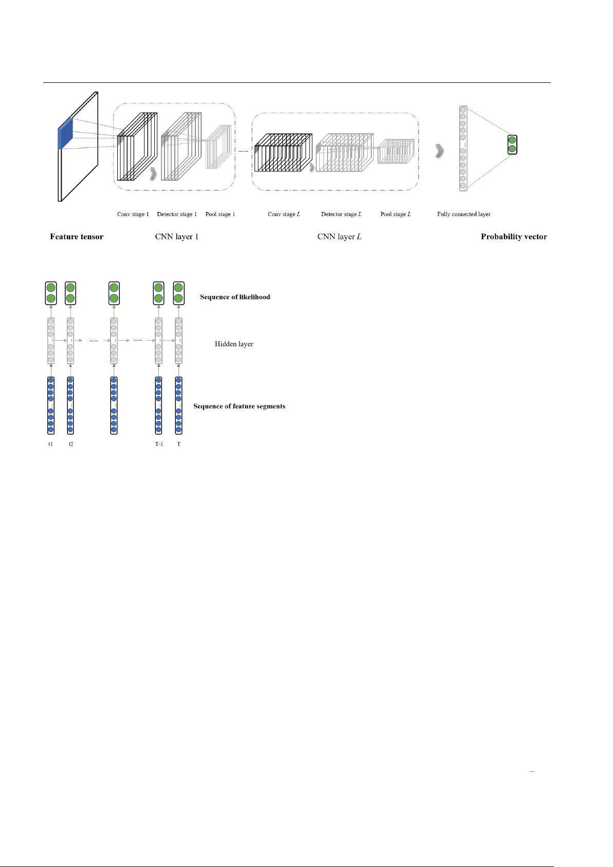
Multimedia Systems man uscript No. (will b e inserted b y the editor) Deep learning-based automatic do wn b eat trac king: a brief review Bijue Jia* · Jianc heng Lv* · Da yiheng Liu* Received: date / Accepted: date Abstract As an important format of multimedia, mu- sic has ﬁlled almost every one’s life. Automatic analyz- ing music is a signiﬁcant step to satisfy p eople’s need for m usic retriev al and m usic recommendation in an eﬀortless wa y . Thereinto, do wn b eat trac king has b een a fundamental and contin uous problem in Music In- formation Retriev al (MIR) area. Despite signiﬁcant re- searc h eﬀorts, down b eat tracking still remains a chal- lenge. Previous researches either fo cus on feature engi- neering (extracting certain features by signal pro cess- ing, which are semi-automatic solutions); or ha ve some limitations: they can only mo del m usic audio record- ings within limited time signatures and temp o ranges. Recen tly , deep learning has surpassed traditional ma- c hine learning metho ds and has become the primary algorithm in feature learning; the com bination of tradi- tional and deep learning metho ds also has made b etter p erformance. In this pap er, w e b egin with a bac kground in tro duction of down beat tracking problem. Then, we giv e detailed discussions of the following topics: sys- tem architecture, feature extraction, deep neural net- w ork algorithms, datasets, and ev aluation strategy . In addition, we take a lo ok at the results from the annual b enc hmark ev aluation–Music Information Retriev al Ev al- uation eXchange (MIREX), as w ell as the developmen ts in softw are implementations. Although muc h has b een ac hieved in the area of automatic down beat trac king, Jiancheng Lv E-mail: lvjiancheng@scu.edu.cn Bijue Jia E-mail: jiabijue@outlo ok.com Da yiheng Liu E-mail: losinuris@gmail.com * College of Computer Science, Sic h uan Univ ersity , Chengdu, P eople’s Republic of China some problems still remain. W e p oint out these prob- lems and conclude with possible directions and c hal- lenges for future researc h. Keyw ords Music down beat tracking · Music In- formation Retriev al · Deep learning · Multimedia · Review 1 In tro duction Music is explicitly structured in a temp oral manner. The time structure of a m usic piece is often conceiv ed as a superp osition of m ultiple hierarc hical lev els or time- scales [65]. People can synchronize with these temp oral scales while playing instrumen ts or dancing. The men- sural level of these temp oral structures (which people tap their feet to) contains the approximately equally spaced b e at , which is the basic unit of time and pulse (regularly rep eating even t) in music theory . Another highly-related term is tatum , whic h is the low est regu- lar pulse train that a listener intuitiv ely infers from the timing of p erceived musical even ts (i.e. a time quan- tum). According to music’s metrical structure, the same amoun t of beats are segmen ted sequen tially into groups called b ars or me asur es . The ﬁrst beat of eac h bar pla ys a role of accentuation, and it is deﬁned as a downb e at . Do wnbeats are often used b y comp osers and conductors to help musicians read and na vigate in a musical piece and by music fans and amateurs to b etter learn music. Automatically analyzing and estimating down beat is of signiﬁcan t importance when w e are trying to analyze and follo w a music piece. The research area that inv estigates computation mo d- els for trac king do wnbeats is known as A utomatic down- b e at tr acking (also called down beat detection or down- b eat estimation). The goal of down beat trackin g is to 2 Bijue Jia* et al. automatically annotate the time points of all the down- b eats in a piece of music audio. An e xample of a song’s annotation ﬁle is shown in Fig. 1. It is useful for v ar- ious tasks such as music audio transcription [11, 90, 91, 98], chord recognition [16, 78], structure segmenta- tion [68, 75, 79, 82, 89] and musicology analysis. Auto- matic do wn b eat tracking can also b e used in music information retriev al [19, 21] and music recommenda- tion [8, 81, 103]. This problem has long b een paid at- ten tion to in the comm unit y of Music Information R e- trieval (MIR, which is an interdisciplinary researc h ﬁeld fo cusing on searching and obtaining information from m usic. Related bac kground knowledge include, but not limited to, musicology , psychology , signal pro cessing, informatics, statistical learning and mac hine learning 1 .) Automatic do wn b eat trac king has also attracted world- wide scholars to exert their eﬀorts to and has b een one of the c hallenging tasks of Music Information Re- triev al Ev aluation eXchange (MIREX) [21] in recen t y ears. The level of current interest b y its recen t inclu- sion in automatic down b eat tracking problem amongst the communit y is illustrated and compared in the MIREX ev aluation initiative. The most similar task related to do wnbeat trac king is b eat trac king [13, 34, 38, 41, 42, 88], whic h has b een studied muc h longer than down b eat trac king. A few researchers are also studying these t w o tasks together [5, 60, 60, 62, 83]. T racking b eats is diﬃ- cult, ho wev er tracking down beats is comparably hard. Do wnbeat trac king problem has been studied from v ery earlier. The premier one prop osed by [43] mo d- els three metrical levels and is reported to successfully trac k do wnbeats in 4/4 m usic with drums, ho wev er, it is built up on hand-designed features and patterns. Un- fortunately , annotating down beat p ositions man ually is a time-consuming and exp ensive pro cess and heav- ily dep ends on the intuition of the developer. Hand- crafted features and rules are also not readily av ailable for most music recordings [14, 25]. A general trend is to divert the atten tion to automatical metho ds. Later systems start to go from hand-crafted features to auto- matically learned ones. One line uses probabilistic state- space models, where rhythmic patterns are learned from data and used as an observ ation mo del [58, 60, 83]. An- other line uses Support V ector Machines (SVMs) to trac k do wnbeat in a semi-automatic setting [55], and later transforms into a fully automatic system with a few b eat-synchronous hand-annotated features. The system of [14] tracks b eats ﬁrst and then calculates the Kullback-Leibler div ergence b et w een tw o consecu- tiv e band-limited beat synchronous spectral diﬀerence 1 F or a more comprehensive survey of MIR, containing bac kground, history , fundamentals, tasks and applications, w e refer readers to the ov erview by [7, 19, 20, 99]. frames to track do wnbeats. P apadop oulos and P eeters [80] join tly trac ks c hords and do wn b eats b y decoding a se- quence of b eat-synchronous chroma vectors using Hid- den Mark o v Mo del (HMM). There are some problems exist in these systems as well: they are applicable to only sev eral simple metrical structures [32, 58], or lim- ited m usical styles [53, 60, 96], or restrictiv e prior kno wl- edge [2, 14, 80]. Systems that forecast some necessary in- formation b eforehand are naturally prone to error prop- agation. Recen t studies resort to deep learning to try to solv e the ab ov e problems. As the amount and v ariousness of data increases, designing features and rules manu- ally is infeasible. Deep learning can obtain higher-level and abstract musical represen tations that fully charac- terize the complexity of the problem that is hard to design by hand. Many of these factors of v ariation can b e iden tiﬁed only through sophisticated, nearly h uman- lev el understanding of m usic. Deep learning solv es this problem by introducing representations that are ex- pressed in terms of other, simpler representations [36]. The adven t of deep learning has had a signiﬁcan t im- pact on many areas in mac hine learning and informa- tion retriev al, dramatically improving the state-of-the- art in tasks such as ob ject detection, image classiﬁca- tion, sp eech recognition, and language translation. Re- cen t years hav e also witnessed a deluge of researches in m ultimedia processing by using deep learning, suc h as music recommendation, multimedia lab eling and re- triev al [77, 101, 102, 107]. As an imp ortant and v aluable t yp e of mu ltimedia, music can also b e well analyzed by deep learning. The quintessen tial mo dels of deep learn- ing are m ultifarious deep neural net works (DNNs). This surv ey fo cuses on DNN-based music do wn b eat track- ing, which has ac hieved in triguing and eﬀective results [5, 22 – 24, 59]. Do wnbeat trac king problem is a bit similar to classi- ﬁcation or sequence lab eling problem [46], whose aim is to annotate a tag to each segment of the original audio sequence. F rom an ov erall persp ective, a typical DNN- based automatic down beat trac king system comprises three ma jor phrases: data prepro cessing, feature learn- ing and temp oral deco ding. An ensemble paradigm of the down b eat trac king system is shown in Fig. 2. More particularly , data prepro cessing can b e separated into t wo procedures called segmentation and feature extrac- tion, and after feature learning, there is a small pro ce- dure called feature com bination. Step b y step, all of the pro cedures are: Segmen tation : In all do wnbeat tracking systems, segmen tation w ould b e the ﬁrst step. By doing so mak es it muc h easier for subsequent stages to detect down- b eats b ecause it does not ha ve to deal with tempo Deep learning-based automatic down beat tracking... 3 Fig. 1 Example of a typical down beat annotation ( Albums-A naBelen V eneo-01.b e at from Bal lr o om dataset), showing down- b eat time (in red dashed line). or expressive timing on one hand and it greatly re- duces the computational complexit y b y both reducing the sequence length of an excerpt and the searc h space. Do wnbeat trac king is then reduced to a classiﬁcation or sequence labeling problem where each segmen t is de- cided as a do wnbeat or not. F eature Extraction : After segmenting, every piece of the fragmen t is a p ossible candidate of a down beat. The ﬁrst thing to do, is amplifying and extracting some signal features so that the latter learning algorithm could capture the c haracteristic easily . In western mu- sic, the down beats usually coincide with chord changes or harmonic cues, whereas in non-western music the start of a measure is often deﬁned b y the b oundaries of rh ythmic patterns. Therefore, many algorithms exploit one or more of these features to trac k the down b eats [5]. The most likely attributes–which are decided manu- ally using domain-sp eciﬁc knowledge of m usic–that con- tribute to the p erception of down b eats are harmony , tim bre, bass conten t, rh ythmic pattern, the lo cal sim- ilarit y in timbre and harmony and p ercussion. Among them, six attributes (harmon y , timbre, bass conten t, rh ythmic pattern, the lo cal similarit y in tim bre and harmon y) con tribute to the grouping of b eats into a bar; tw o attributes (harmon y and p ercussion) are b eat- sync hronous features. F eature Learning : The extracted features are then running through the DNN. If features are more than one kind, each of them is sent to indep endent neural net- w orks as input, and these netw orks are called feature adapted neural net w orks. This is a conv enient approach to work with features of diﬀeren t dimension and assess the eﬀect of each of them. More detailed illustration ab out DNN-based feature learning metho ds will b e dis- cussed in Section 3. F eature Com bination : As it is imp ortant for the follo wing deco ding pro cess to reduce estimation errors, leading to a tradeoﬀ among the outputs from diﬀerent feature adapted neural netw orks. Durand et al. [22] use an av erage of the observ ation probabilities obtained by those indep endent netw orks. The av erage or sum rule is in general quite resilien t to estimation errors [57]. T emp oral Deco ding : T emp oral deco ding stage is the last step of a down b eat tracking system; it an- alyzes a do wn b eat likelihoo d sequence which is out- put by DNNs and maps the sequence in to a discrete sequence of down beats. Commonly-used metho ds are Hidden Mark ov Mo del (HMM) and Dynamic Bay esian Net work (DBN). Krebs et al. [59] hav e exp erimented and prov ed that an added DBN stage is p erforming b etter than a simple DNN output (i.e. simply rep orts do wnbeats if the output likelihoo d of DNN activ ations exceeds a threshold). In Section 4 w e will give a detailed description of eac h algorithm. Consequen tly , to give researchers a clear understand- ing of DNN-based automatic down beat tracking sys- tem, this review expatiates eac h step of the system as comprehensiv e as p ossible. More imp ortantly , this pa- p er fo cuses on three diﬀerent general DNN architec- tures during the feature learning step and makes a brief comparison among them. Additionally , we further go through some work and information that are inv olved in do wnbeat tracking researches. The remainder of this pap er is organized as follo ws. Section 2 gives an o v erview of the segmen ts and segmen- tation metho ds for prepro cessing. In Section 3, we will summarize all the features that correlate to down b eats and their extraction metho ds. Common and general DNN mo dels are depicted in Section 4. In the follow- ing Section 5, sev eral frequently used temp oral decod- ing and machine learning algorithms will b e summed- up. Section 6 gives a complete list of datasets used for do wnbeat trac king problem. Some commonly-used ev al- uation methods are discussed in Section 7. Then in Sec- tion 8 describ es an incomplete list of the most relev ant soft ware pack ages or libraries to down beat tracking. Fi- nally , Section 9 discusses the prev alen t metho ds and what the probable future directions are and what the most c hallenging issues could be. This surv ey is struc- tured logically rather than c hronologically . 4 Bijue Jia* et al. Fig. 2 General architecture for down b eat trac king systems. 2 Segmen ts and Segmen tation Metho ds The goal of m usic audio segmen tation is to switc h down- b eat annotation problem to sequence lab eling problem. Finding the exact timestamp of a down beat is imp os- sible because time is con tin uous. Instead, w e can split m usic audio into a sequence of s mall segments and de- cide eac h segmen t is a do wn b eat or not. If a segmen t is a do wnbeat, then use the o ccurrence time of this segment as the annotation of this down beat. Doing segmentation is desirable b ecause temp o-inv arian t features decrease the capacity and simplify the feature learning pro cess while making it less prone to o v er-ﬁtting [22]. There are three kinds of segments that are commonly used in do wnbeat tracking: b eat segmen t, tatum segment, and frame segmen t. Beat Segmentation : Durand et al. [22] and Krebs et al. [59] temp orally segment the signal into subdivi- sions of the rhythmic beat. They seek the segmentation that maximizes do wnbeat recall rate while emphasiz- ing consistency in inter-segmen t durations. T o ac hiev e these goals they extend the lo c al pulse information ex- tr actor presented in [47] and process the following op- erations: a) First, they use this to olb ox to obtain a temp ogram of the musical audio. b) Then they use dy- namic programming with strong contin uit y constraints and emphasis to w ards high tempi. c) Finally they use the deco ded path to recov er instantaneous phase and amplitude v alues, construct the predominant lo cal pulse (PLP) function as in [47], and detect pulses using peak- pic king [18]. Using this pro cedure, the recall rate for do wnbeat pulses is ab ov e 95% for each dataset, using a 100 ms tolerance windo w. T atum Segmentation : Durand et al. [23,24] adopt the lo c al pulse information extr actor prop osed to ac hiev e a useful tatum segmen tation. The Processing procedure is: a) C omputing the temp ogram of the m usical audio through a Short-T erm F ourier T ransform (STFT) and only keep the tempo ab o ve 60 rep etitions p er minute to a v oid slo w metrical lev els. b) T rac king the best pe- rio dicit y path by dynamic programming with the same kind of lo cal constraints. The following system can ﬁnd a fast sub division of the down b eats at a rate that is lo cally regular. c) Finally using the deco ded path to re- co ver instan taneous phase and amplitude v alues, con- struct the PLP function, and detect tatums using p eak- pic king on the PLP . The resulting segmentation p erio d is typically twice as fast as the b eats p erio d, while it can b e up to four times faster. F rame Segmentation : B¨ oc k et al. [5] use a v ery simple wa y to do segmentation. They split audio into o verlapping frames, with 100 frames p er second (100 fps), implying that tw o neigh b oring frames are lo cated 10ms apart. This is also the initial pro cessing stage of STFT. Unlike beat and tatum, a frame is not as a lo w-level music c haracteristic but as a raw audio piece. Using frame segmen tation av oids hand-crafted features suc h as harmonic change detection [22, 23, 25, 56, 80], or rhythmic patterns [53, 54, 60]. The relev an t features can b e learned directly from the sp ectrogram, therefore frame segmentation shows up in pair with auto-learned features, and should co-op erate with DNN-based fea- ture learning algorithms (will b e discussed in section 3.9 and section 4). Deep learning-based automatic down beat tracking... 5 3 F eatures and F eature Extraction Algorithms Finding musical features that correlate to do wn beat is v ery helpful since these attributes mak e learning al- gorithms or classiﬁers to app erceive down b eats more easily . It is worth mentioning that in most cases hand- crafted feature w orks well when the dataset is not large, homogenous, high-qualiﬁed or identically-distributed. By doing features extraction, the dimension of data is reduced, so that learning algorithms could b e less com- plicated and run faster. In this section, w e summarize the most relev ant features to down b eats and their cor- resp onding extraction metho ds. 3.1 Harmon y In m usic, harmony considers the pro cess b y whic h the comp osition of individual sounds, or sup erp ositions of sounds, is analyzed b y hearing. Usually , this means si- m ultaneously occurring frequencies, pitches (tones, notes), or chords [69]. Change in harmony or timbre con tent (will b e describ ed in section 3.3), for example, c hord c hanges, section changes or the entrance of a new in- strumen t is often related to a down b eat p osition [22]. The feature of harmon y is represented by chroma [3]. There are tw o main w ays of extracting harmony . One wa y is used by Durand et al. [22, 24] and they extracts the harmonic feature as the following steps: 1)First, they down-sample the audio signal at 5512.5 Hz. 2)They then compute the STFT using a Hann win- do w of size 4096 and a hop size of 512. 3)They ap- ply a constan t-Q ﬁlter-bank with 108 bins (36 bins p er o cta ve). 4)The y conv ert constant-Q sp ectrum to har- monic pitch class proﬁles 5)Afterward, they remov e o c- ta ve information by accum ulating the energy of equal pitc h classes. 6)They tune the chromagram b y ﬁnding bias on peak lo cations; smooth it b y a median ﬁlter of length 8. 7)In the end, they map it to a 12 bins rep- resen tation by av eraging. The other wa y is conducted b y Krebs et al. [59] and they use the CLP c hroma fea- ture [76] with a frame rate of 100 frames p er second. Then they sync hronize the features to the b eat by com- puting the mean v alue ov er a windo w of length 4 b/n h ( 4 b is the b eat p erio d), yielding n h = 2 feature v alues p er b eat in terv al. 3.2 Harmon y Similarity By lo oking at harmony similarit y or timbre similarit y (detailed description is in section 3.4), we can observe longer-term patterns of change and no v elty that are in- v ariant to the sp eciﬁc set of pitch v alues or sp ectral shap e. The similarity in harmony , for example, has the in teresting prop erty of b eing key inv ariant and there- fore can mo del cadences and other harmonic patterns related to down b eat p ositions [22]. The feature of har- mon y similarit y is represen ted by c hroma similarit y (CS). The chromas are computed the same as in section 3.1, but they are then av eraged to obtain segment syn- c hronous c hroma. F or eac h segmen t, compute the cosine similarit y of one segment synchronous chr oma with the 24 segment synchronous chroma around it. The dimen- sion of CS is 24. 3.3 Tim bre In music, timbre is the p erceived sound quality of a m usical note, sound or tone. Timbre distinguishes dif- feren t types of sound pro duction, such as choir v oices and musical instruments. Alternations of the timbre- inspired conten t o ccur more likely at the start of a new section and near a do wnbeat position [24]. the feature of tim bre is represen ted b y Mel-frequency cepstral co- eﬃcien ts (MFCC). Tim bre extraction can also b e done in conjunction with an onset [55], tatum or b eat seg- men tation [24]. Durand et al. [22] compute the ﬁrst 12 Mel-frequency cepstral co eﬃcien ts using [1], with a Hamming window of size 2048, a hop size of 1024 and 32 Mel ﬁlters on a signal sampled at 44100 Hz. 3.4 Tim bre Similarity The feature of tim bre similarity is represen ted b y MF CC similarit y (MS). The MF CC sp ectrograms are computed the same as in section 3.3, but they are then av eraged to obtain segment synchronous MFCC sp ectrogram. F or each segment, computing the cosine similarity of one segment-sync hronous MFCC sp ectrogram with the 24 segmen t-sync hronous MF CC sp ectrogram around it. The dimension of MS is 24. 3.5 Bass Con tent The bass conten t is low-frequency , containing mostly bass instrument or kic k drum, b oth of which tend to be used to emphasize the down b eat [22]. The feature of lo w-frequency conten t is represented b y low-frequency sp ectrogram (LFS). Durand et al. [22,24] compute LFS as follows: 1)First they downsample audio signal at 500 Hz. 2)Then they compute STFT by a Hann window of size 32 and a hop size of 4 to get the sp ectrogram. 3)They keep the 6 Bijue Jia* et al. sp ectral comp onents below 150 Hz (the ﬁrst 10 bins). 4)Finally , they clip the signal so that all v alues on the 9th decile are equal. 3.6 Rh ythmic Pattern Rh ythm is the timing of musical sounds and silences that o ccur ov er time. Rhythmic patterns are frequently rep eated eac h bar and are therefore useful to obtain the bar b oundaries. The feature of the rhythmic pattern is represen ted by onset detection function (ODF). Durand et al. in their early work [22] use 4 band- wise ODF as computed b y [58]. First, they compute the STFT using a Hann window of size 1024 and a hop size of 256 for a signal sampled at 44100 Hz. Second, they compute the sp ectrogram and apply a 36-bands Bark ﬁlter. Third, they use µ -law compression with µ = 100 and downsample the signal by a factor of t wo. F ourth, they do env elope detection using an order 6 Butter- w orth ﬁlter with a 10 Hz cutoﬀ. Fifth, a w eigh ted sum of 20% of the env elop e and 80% of its diﬀerence is done to compute the ODF. Finally , they map ODF to 4 equally distributed bands. Durand et al. in their later work [23, 24] compute a 3-band sp ectral ﬂux ODF: 1)They perform STFT to get the spectrogram. 2)They apply µ -law compression with µ = 10 6 to the STFT co eﬃcients. 3)They sum the discrete temp oral diﬀerence of the compressed signal on 3 bands for each temporal interv al, and subtract the lo cal mean and half wa ve. The frequency interv als of the low, medium and high-frequency bands are [0 150], [150 500] and [500 11025] Hz resp ectiv ely . 3.7 Melo dy A melody is a linear succession of m usical tones that the listener p erceives as a single en tit y; it is a combination of pitch and rhythm. F or melo dy , some notes tend to b e more accented than others and b oth pitch con tour and note duration pla y imp ortan t roles in our in ter- pretation of meter [26, 50, 84]. The feature of melo dy is represen ted by melodic constan t-Q transform (MCQT). Durand et al. [23, 24] get melo dy features as follo ws: 1)They do wnsample audio at 11025 Hz. 2)They conduct STFT with Hann window of size 185.8 ms and hop size 11.6 ms. 3)They apply a constant-Q transform (CQT) with 96 bins per o ctav e, starting from 196 Hz to the Nyquist frequency to the STFT, and a verage the energy of eac h CQT bin q[k] with the following o ctav es: s [ k ] = P J k j =0 q [ k + 96 j ] J k + 1 (1) with J k suc h that q [ k + 96 J k ] is b elow the Nyquist fre- quency . 4)Then they only keep 304 bins from 392 Hz to 3520 Hz that corresp ond to 3 o ctav es and 2 semi- tones. 5)They use a logarithmic represen tation of s to represen t the v ariation of the energy more clearly: r = log ( | ˆ s | + 1) (2) where ˆ s is the restriction of s b etw een 392 Hz and 3520 Hz. 6)They set ev ery v alue whic h is under the 3rd quar- tile Q 3 of a giv en temporal frame to zero to get the ﬁnal melo dic CQT: m C QT = max ( r − Q 3 ( r ) , 0) (3) 3.8 P ercussion P ercussion is commonly referred to as ”the bac kbone” or ”the heartbeat” of a m usical ensem ble, often w ork- ing in close collab oration with bass instruments, when presen t. Krebs et al. [59] compute a m ulti-band sp ectral ﬂux: 1)First, they compute the magnitude sp ectrogram b y applying the STFT with a Hann window, hop size of 10ms, and a frame length of 2048 samples. 2)Second, they apply a logarithmic ﬁlter bank with 6 bands p er o cta ve, cov ering the frequency range from 30 to 17 000 Hz, resulting in 45 bins in total. 3)Third, they com- press the magnitude b y applying the logarithm. 4)F or ev ery frame, they compute the diﬀerence b etw een the curren t and the previous frame. 5)Finally , they b eat- sync hronize the feature sequence by only keeping the mean v alue p er frequency bin in a windo w of length 4 b/n p , where 4 b is the b eat p erio d and n p = 4 is the n umber of b eat sub divisions, centered around the b e- ginning of a b eat sub division. 3.9 Auto-learned F eatures The selection of appropriate features is a diﬃcult task. Researc hers are frequently unsure about which features are useful, and it is diﬃcult to extract the p erfect fea- tures. Although researchers generally just formulate a limited hypothesis ab out which type of features may b e suitable according to their exp erience and domain kno wledge, this may lead to p o or p erformance b ecause of the limitation of their hypothesis. Sp on taneously , we ma y w ant machine itself to automatically ﬁnd out which features are related to do wnbeat. A study of automatic extracting features has con- ducted by [5], who av oids hand-crafted features but prefer the algorithm to learn some relev ant features di- rectly from sp ectrograms. These spectrograms are ob- tained as follo ws: 1)Splitting audio signal ov erlapping Deep learning-based automatic down beat tracking... 7 frames and weigh ted with a Hann window of the same length before being transferred to a time-frequency rep- resen tation with STFT. Tw o adjacen t frames are lo- cated 10 ms apart, which corresp onds to a rate of 100 fps (frames per second). 2)Omitting the phase p ortion of the complex spectrogram and use only the mag- nitudes for further pro cessing. 3)Using three diﬀeren t magnitude sp ectrograms with STFT lengths of 1024, 2048, and 4096 samples (at a signal sample rate of 44.1 kHz). 4)Limiting the frequencies range to [30, 17000] Hz to reduce the dimensionalit y of the features. 5)Pro- cessing the spectrograms with logarithmically spaced ﬁlters. A ﬁlter with 12 bands p er octav e corresponds to semitone resolution, which is desirable if the har- monic con tent of the sp ectrogram should b e captured. 6)Using ﬁlters with 3, 6, and 12 bands p er o ctav e for the three spectrograms obtained with 1024, 2028, and 4096 samples, respectively , accoun ting for a total of 157 bands. 7)Scaling the resulting frequency bands logarith- mically to b etter match human p erception of loudness. 8)Adding the ﬁrst order diﬀerences of the sp ectrograms to the features. The ﬁnal dimension of the features 314. 4 DNN-Based F eature Learning Algorithms So far, we ha v e introduced down beat-related music fea- tures. The aforementioned features can directly ﬂow in to the temp oral deco ding pro cedure to get the ﬁnal results, as some systems do [10, 27 – 30, 71]. This w orks w ell when data is little, but as the num b er of data in- creases, the diversit y and complexity of data also grow and some weak p oin ts may app ear. Under this circum- stance, the DNN-based feature learning algorithms are inserted in b etw een the feature extraction and temporal deco ding pro cedures to further extract and learn fea- tures. The diﬀerences b et ween systems with and with- out DNN pro cess exist in sev eral asp ects: – The fundamental feature extraction algorithms learn more low-lev el features, while DNN-based feature learning algorithms disco ver more high-lev el and ab- stract features. – The aforementioned features are hand-crafted and empirically-based which heavily resort to prior kno wl- edge of exp erts and need a very long p erio d to ver- ify eﬀectiv eness, while features learned b y DNNs are automatically-extracted which rely on the strength of big data and can b e v eriﬁed quickly . – More human prejudices exist in features designed b y exp erts but less in those extracted by learning algorithms. Note that features disco vered by learn- ing algorithms may not in sync with our common Fig. 3 Sketc h diagram of a deep feed forw ard net work. sense, how ever they pla y a vital role in impro ving mo del p erformance. – Using DNN enlarges the num b er of parameters so that the represen tation is more p ow erful. In the following, w e will describ e and compare three diﬀeren t DNN algorithms. These are the three main mo dels used in feature learning part: Multi-La y er Per- ceptron (MLP), Con volutional Neural Netw ork (CNN) and Recurren t Neural Netw ork (RNN). 4.1 Multi-La yer Perceptron Multi-La yer P erceptron, or deep feedforward net work, is the quin tessen tial deep learning mo del. In some pa- p ers, it is also called the general DNN [22]. In order not to cause ambiguit y , we refer to MLP instead of DNN when w e talk about this algorithm. While playing the role of feature learner in down b eat tracking problems, MLP is a series of functions to estimate the probabil- it y of a feature being a down b eat. A sketc h diagram of MLP is shown in Fig. 3. An MLP is a cascade of L la yer functions of performing linear and non-linear transfor- mations successiv ely . The l -th lay er functions are: z l = x l − 1 W l − 1 + b l − 1 , (4) f l ( x l ; θ l ) = ϕ ( z l ) , θ = [ W l ; b l ] (5) where x l ∈ R d with dimension d is the input down b eat feature v ector when l = 1, and the output v alue of la yer l − 1 when l > 1. ϕ is the non-linear transformation function (e.g. sigmoid, ReLU [35], maxout [37], etc.). θ l represen ts the l -th la yer parameters; W l ∈ R d × d l is a matrix of weigh ts; b l ∈ R d l is a vector of biases; d l is the dimension of lay er l . At L -th lay er (the output la yer), ϕ is normally the sigmoid function: sig moid ( z L ) = 1 1 + e − z L , (6) 8 Bijue Jia* et al. or the softmax function: sof tmax ( z L ) i = exp ( z L ) i P K k =1 exp ( z L ) k . (7) where K is the dimensionalit y of the output la yer and also is the n um ber of classes we w ant to detect. Sigmoid can only b e used for binary classiﬁcation issue, while softmax can deal with more than t wo classes. Both of them output conditional probabilities P( x 1 | Θ ). As for do wnbeat trac king problem, sigmoid function just giv es the probability of one feature x 1 b eing a down b eat (i.e. do wnbeat lik eliho o d), while softmax giv es ev ery proba- bilit y of one feature b elonging to each class. 4.2 Con volutional Neural Netw orks Con volutional Neural Net w orks are simply neural net- w orks that use conv olution in place of general matrix m ultiplication in at least one la y er [36]. A typical CNN la yer consists of three stages sequentially: conv olution stage, detector stage, and p o oling stage [36]. The com- plete CNN includes stack ed conv olutional and po oling la yers, at the top of which are multiple fully-connected la yers. A sketc h diagram of CNN is shown in Fig. 4. 4.2.1 Convolution Stage Giv en input do wn b eat features X ∈ R c × w × h with c han- nel n umber c , feature width w (could b e time length), and feature height h (could be frequency bandwidth), the con v olutional la y er con v olv es X with K ﬁlters (or called kernels ) where each ﬁlter W k ∈ R c × m × n is a 3- dimensional tensor with width m and height n . W e will obtain K feature maps, which constitute a 3-dimensional tensor Z ∈ R K × w Z × h Z . The k -th feature map Z k is computed as follo ws: Z k = X ∗ W k + b k , k = 1 , · · · , K . (8) where ∗ denotes the con volution operation and b k is a bias parameter. The conv olution on X is operated not only along the feature height (frequency) axis but also along the feature width (time) axis, which results in a simple 2-dimensional conv olution commonly used in computer vision. 4.2.2 Dete ctor Stage Before doing the p o oling part, we often operate an elemen t-wise non-linear function on the feature maps w e obtain after con volution. Here we also denote ϕ as the non-linear function, and transform feature maps Z to A : A = ϕ ( Z ) (9) 4.2.3 Po oling After the element-wise non-linearities, feature maps are passed through a p o oling lay er. A p o oling function re- places the neuron v alues of the feature map at a certain lo cation with a summary statistic of the nearby neuron v alues. The most frequen tly-used p o oling function is max p o oling. The max p o oling [106] op eration reports the maxim um output within a rectangular neighborho o d. With regard to the k -th activ ated feature map A k , the v alue at p osition ( t, r ) of the after-p o oling feature map S k is computed b y: [ S k ] t,r = max p i =1 { [ A k ] t × s + i,r × s + i } (10) where s is the step size and p is the p o oling size. Other p opular p o oling functions include the a verage of a rect- angular neigh b orho o d, the L2 norm of a rectangular neigh b orho o d, or a w eighted a verage based on the dis- tance from the central pixel. W e do p o oling only along the frequency axis since it helps to reduce spectral v ari- ations while p o oling in time has b een shown to b e less helpful [86]. On the top of the complete CNN, fully-connected la yers are applied. Their structures are simply the same as the aforementioned MLP . The input to this fully- connected la y er is a concatenation of all ﬂattened fea- ture maps S k . The output is the do wnbeat likelihoo d. 4.3 Recurren t Neural Netw orks Recurren t neural netw orks or RNNs [85] are a family of neural net w orks for pro cessing sequential data. Muc h as a CNN is a neural netw ork that is spec ialized for pro cessing a grid of v alues X such as an image, an RNN is a neural netw ork that is sp ecialized for pro cessing a sequence of v alues x 1 , · · · , x T . Considering the down b eat feature as a s equence X = [ x 1 , · · · , x T ] > , in this w a y , down beat tracking can b e seen as a sequence lab eling problem. V ector x t is in- dexed with time step t , ranging from 1 to T . A one- hidden-la yer v anilla RNN is comp osed of three la yers: an input lay er, a hidden lay er, and an output lay er. Computation runs along b oth lay er axis and time axis. A one-hidden-la y er v anilla RNN is sho wn in Fig. 5. The hidden la yer at time t is computed as: h t = f h ( x t W ih + h t − 1 W hh + b h ) (11) where f h is the hidden lay er activ ation function, W ih is the w eigh t matrix connecting input la yer and hid- den lay er, W hh is the w eight matrix betw een adjacen t time-step hidden lay ers (i.e. this weigh t matrix is shared Deep learning-based automatic down beat tracking... 9 Fig. 4 Sketc h diagram of a deep conv olutional neural netw ork. Fig. 5 Sketc h diagram of a one-hidden-lay er recurren t neural netw ork. along the time axis) and b h is the bias v ector of the hid- den units. F ormula 11 is also called the basic RNN unit. Output la yer at time t is computed as: y 0 t = f o ( h t W ho + b o ) (12) where f o is the output la y er activ ation function, W ho is the w eight matrix b etw een hidden lay er and output la yer and b o is the bias v ector of the output units. Practically , v anilla RNN is not p erforming w ell cause its gradien t v anishing and explo ding issue. More so- phisticated and p ow erful RNN units include Long-Short T erm Memory (LSTM) [52], Gated Recurren t Unit (GRU) [9] etc. If f o is sigmoid function, at time t output y t is a scalar; the whole output sequence y 0 = [ y 0 1 , y 0 2 , · · · , y 0 T ] represen t the do wn b eat lik eliho o d. If f o is softmax func- tion and tw o classes (do wn beat and non-do wnbeat) to b e classiﬁed, output y 0 t ∈ R 2 at time t is a vector, con- sisting of the down beat lik eliho o d and non-do wn b eat lik eliho o d v alue. W e take out only the down b eat like- liho o d v alues as the ﬁnal probabilit y sequence y 0 = [ y 0 1 , y 0 2 , · · · , y 0 T ]. Each elemen t of this sequence is the parallel-corresp onding prediction to the input segment sequence. 4.4 Comparison of DNNs on Do wnbeat T racking The preceding text has expatiated three kinds of DNN mo dels and describ ed eac h model independently , ho w- ev er, there are some notable diﬀerences among them when solving down b eat trac king problem. The diﬀer- ences are discussed from sev eral p ersp ectives: – F rom the innate and intrinsic diﬀerence point of view, MLP is more computationally expensive due to its fully-connected architecture. Comparing to MLP , the n um ber of parameters of CNN and RNN is muc h smaller. When the dimension of the down- b eat feature is small, these three mo dels all work w ell. MLP alwa ys is the ﬁrst thought [22] b ecause it’s v ery ﬂexible and the results can b e used as a baseline p oin t of comparison. – Cho osing which mo del to use also dep ends on what basic problem the authors see do wn b eat tracking as. Some researchers view do wn b eat tracking as a se- quence mo deling problem. F eature v alues that fall in to one time unit (beat, tatum or frame) are con- densed into one v ector and all v ectors of one au- dio signal are organized in sequence according to their occurrence time. In this case, RNN is the most suitable model since it is the natural c hoice for se- quence modeling tasks [5, 59]. CNN can also be used to mo del sequence and giv e the probability of eac h comp onen t of a sequence being a down b eat or not, just like the rh ythmic neural netw ork designed by [23]. Some other researchers treat do wn beat track- ing as a binary classiﬁcation problem ﬁrst–let the mo del learn to distinguish which input feature is a down b eat feature and which is not. In this case, MLP and CNN are more suitable mo dels [22 – 24]. 10 Bijue Jia* et al. When seeing it as binary classiﬁcation problem, some of the features at non-down b eat p osition need to b e randomly remov ed in order to obtain an equal amoun t of features computed at down b eat and non- do wnbeat positions [22]. Eac h do wnbeat-correlated m usical feature is considered indep endently and one net work is trained p er feature. Output probabilities obtained b y these indep enden t netw orks are av er- aged or summed in the end and then are organized in a probability sequence. Note that when training these classiﬁers, the temp oral correlation betw een adjacen t features is ignored. Generally sp eaking, when the down beat problem size is small and w e w ant to quickly get a rough result, MLP w ould b e the ﬁrst to try; when we wan t to fo cus on the spatial relationship within features (such as harmony and melo dy features), CNN w ould b e b etter; when w e w ant to model temp oral characteristics while learning features, RNN is the b etter candidate mo del. 5 T emp oral Deco ding Algorithms T emp oral decoding maps the output lik elihoo d sequence of DNN into the discrete sequence of down b eats, incor- p orating m usical prior kno wledge into the pro cess. Two frequen tly-used algorithms are HMM and DBN (in fact, HMM is a simple and sp ecial case of DBN). In this sec- tion, we will describe in detail the tw o algorithms and ho w they solve the last problem. 5.1 Hidden Mark ov Mo del Hidden Marko v Mo del (HMM) is a probability model with resp ect to time series. It describ es a process, where a hidden Mark o v chain randomly generates an invisi- bly random state sequence, and then eac h state gener- ates each observ ation. Supp ose S = { s 1 , s 2 , · · · , s N } is the set of all p ossible states, namely the state space; V = { v 1 , v 2 , · · · , v M } is the set of all p ossible observ a- tions. HMM mo del is comp osed of three comp onents: initial state probability v ector π ∈ R T , state transfor- mation probability matrix A ∈ R N × N and observ ation probabilit y matrix B ∈ R N × M , where T is the time length. So a HMM mo del λ can b e sym b olized as: λ = ( A , B , π ) (13) There are three fundamental problems with regard to HMM: a) probability computation, b) learning prob- lem, and c) deco ding problem. Among them, the decod- ing problem is what w e try to solve at the last step of a do wnbeat tracking system. Decoding problem is deﬁned as this: given mo del λ = ( A , B , π ) and observ ation sequence o = [ o 1 , o 2 , · · · , o T ], ﬁnd the state sequence y = [ y 1 , y 2 , · · · , y T ] so that the conditional probability P ( y | o ) achiev es maximum (i.e. ﬁnd the most p ossibly corresp onding state sequence). 5.1.1 Viterbi Algorithm Viterbi Algorithm is prop osed to solve the deco ding problem of HMM b y us ing dynamic programming. It is using dynamic programming to ﬁnd a path that achiev es maxim um or b est probability; here a path corresp onds to a state sequence. Viterbi algorithm is used to deco de down b eat likeli- ho o d to the most lik ely down b eat state sequence [22– 24]. They mo del the problem as follo ws: 1) State space S = { s 1 , s 2 , · · · , s N } , where N is the n umber of possible states. On the whole, states are par- titioned into tw o distinct states: down beat and non- do wnbeat. It is w orth noting that the do wnbeat lik eli- ho o d dep ends on the bar length and the p osition inside a bar, therefore a state is deﬁned for eac h p ossible seg- men t (b eat or tatum) in a given bar. F or those [22] who segment audio signal in to b eat segments, states corresp ond to do wnbeats and non-down beats in a sp e- ciﬁc metrical p osition. F or example, the do wn b eat in 4/4 and in 5/4 time signatures correspond to diﬀerent states. Likewise, the ﬁrst non-down b eat in 3/4 is diﬀer- en t from its second non-down beat and diﬀerent to any other non-do wnbeat in a diﬀerent meter. F or those [24] who segment audio into tatum segmen ts, time signa- tures of 3,4,5,6,7,8,9,10,12,16 tatums p er bar are al- lo wed. F or example, considering tw o possible bars of t wo and three tatums, there would b e ﬁve diﬀerent states in the mo del. One state represents the ﬁrst tatum of the tw o-tatum bar, and one state represents the sec- ond tatum of the t wo-tatum bar and so forth. 2) State transition probabilit y matrix A = [ a ij ] N × N , where a ij = P ( y t +1 = s j | y t = s i ) , i = 1 , ..., N ; j = 1 , · · · , N is the probability of state s i at time t trans- ferring to state s j at time t + 1. V alues of A needs to b e trained to get (e.g. if a transition from i to j o ccurs q times out of a total Q transitions from i to any state, then a ij = max( q Q , 0 . 02)). 3) Observ ation probabilit y matrix B = [ b j ( k )] N × M , where b j ( k ) = P ( o t = v k | y t = s j ) , k = 1 , · · · , M ; j = 1 , · · · , N is the probability of state s j at time t gen- erates observ ation v k . V alues of b j are distinguished in to tw o cases: a) the state s j corresp onds to a segment (tatum or b eat) at the b eginning of a bar: s j ∈ S 1 ⊂ S , then it is equal to the do wnbeat likelihoo d y 0 ; or b) the state s j corresp onds to another p osition inside a bar: s j ∈ S 1 ⊂ S , then it is equal to the complemen tary Deep learning-based automatic down beat tracking... 11 probabilit y 1 − y 0 : b j = ( y 0 , if s j ∈ S 1 1 − y 0 , if s j ∈ S 1 (14) 4) Initial state probabilit y vector π = [ π i ] 1 × N , where π i = P ( y 1 = s i ) is the probabilit y of y 1 b eing in state s i initially . F or down b eat trac king problem, eac h v alue π i is equally distributed: π i = 1 N , ∀ s i ∈ S . Then we can obtain the ﬁnal down b eat segmen t se- quence follo wing Algorithm. 1 b elow. Algorithm 1 Viterbi Algorithm Input: Mo del λ = ( A , B , π ); observ ation sequence o = [ o 1 , o 2 , · · · , o T ]. Output: Optimal state sequence y = [ y 1 , y 2 , · · · , y T ]. 1: Initialize δ 1 ( i ) = π i b i ( o 1 ) , i = 1 , 2 , · · · , N 2: ψ 1 ( i ) = 0 , i = 1 , 2 , · · · , N 3: for t = 2 , 3 , · · · , T do 4: δ t ( i ) = max 1 ≤ j ≤ N [ δ t − 1 ( j ) a j i ] b i ( o t ) , i = 1 , 2 , · · · , N 5: ψ t ( i ) = argmax 1 ≤ j ≤ N [ δ t − 1 ( j ) a j i ] , i = 1 , 2 , · · · , N 6: end for 7: P ∗ = max 1 ≤ i ≤ N δ T ( i ) 8: y T = argmax 1 ≤ i ≤ N [ δ T ( i )] 9: for t = T − 1 , T − 2 , · · · , 1 do 10: y t = ψ t +1 ( y t +1 ) 11: end for 12: return optimal sequence y = [ y 1 , y 2 , · · · , y T ]; 5.2 Dynamic Ba yesian Netw ork Dynamic Ba yesian Netw ork (DBN) is the generalization of HMM. It is adept at dealing with ambiguous RNN observ ations and ﬁnds the global b est state sequence giv en these observ ations. DBN can use the Most Prob- able Explanation (MPE) feature to ﬁnd the most prob- able state sequence. The pro cess is analogous to the Viterbi algorithm with HMM, ho wev er, is more gen- eral. [5, 59] use DBN as the temp oral decoding algo- rithm and they mo del the problem as follo ws: 1) State space S = { s 1 , s 2 , · · · , s N } . A state s ( b, r ) is the DBN state space is determined by t w o hidden state v ariables: the b eat coun ter b and the time signature r The b eat counter counts the b eats within a bar b ∈ { 1 , · · · , N r } where N r is the num b er of b eats in time signature r (e.g. r ∈ { 2 / 4 , 3 / 4 , 4 / 4 } for the case where a 3/4 and a 4/4 time signature are mo delled). 2) State transition probabilit y matrix A = [ a ij ] N × N . Elemen t a ij = P ( s k | s k − 1 ) is decomp osed via: P ( s k | s k − 1 ) = P ( b k | b k − 1 , r k − 1 ) . . . P ( r k | r k − 1 , b k , b k − 1 ) (15) where P ( b k | b k − 1 , r k − 1 ) = ( 1 , if b k = ( b k − 1 mod r k − 1 ) + 1 0 , otherwise (16) This forces that b eat counter only mov es steadily from left to right in a bar. Time signature c hanges are only allo wed to happen at the be ginning of a bar (i.e. b k < b k − 1 ), so the probabilit y is deﬁned as: if b k < b k − 1 P ( r k | r k − 1 , b k , b k − 1 ) =    1 − p r , if r k = r k − 1 p r R , if r k 6 = r k − 1 else P ( r k | r k − 1 , b k , b k − 1 ) = 0 (17) where p r is the probability of a time signature change; it is learned on the developmen t set and [59] ﬁnds out that p r = 10 − 7 is an ov erall go o d v alue, which mak es time signature c hanges improbable but p ossible. 3) Observ ation probabilit y matrix B = [ b j ( k )] N × M , where b j ( k ) = P (features k | s j ) is the probabilit y of state s j at time t generates observ ation v k . It can be obtained b y rescale the do wn b eat lik eliho o d y 0 = P ( s j | features k ) through: P (features k | s j ) ∝ P ( s j | features k ) P ( s j ) (18) 4) Initial state probability vector π is a uniform distribution o ver the states. 6 Datasets In this section, we review the data av ailable to down- b eat tracking researches and discuss t wo tec hniques to divide datasets for training. 6.1 Av ailable Datasets Datasets 2 used for training and ev aluation are listed in T able 1. They are: 2 A more complete list of datasets for MIR research is at: http:// www.audio conten tanalysis.org/data-sets/ 12 Bijue Jia* et al. T able 1 Overview of the av ailable datasets for Down beat T racking research Dataset Reference # excerpts T otal length Source Ballroom [45, 60] 685 5h 57m http://m tg.upf.edu/ismir2004/contest/tempoContest/node5.html https://gith ub.com/CPJKU/Ballro omAnnotations Beatles [12, 51] 180 8h 09m http://www.isophonics.net/con tent/reference-annotations- beatles Carnatic [95, 97] 176 16h 38m http://compm usic.upf.edu/carnatic-rhythm-dataset Cretan [54] 42 2h 20m Not publicly av ailable GTZAN [70, 100] 1000 8h 20m http://anasyn th.ircam.fr/home/media/GTZAN-rhythm/ http://www.marsy as.info/temp o/ Hainsworth [48, 49] 222 3h 20m http://www.marsy as.info/temp o/ HJDB [53] 236 3h 19m h ttp://ddmal.music.mcgill.ca/breakscience/dbeat Klapuri [58] 320 4h 54m http://www.cs.tut.ﬁ/ ˜ klap/iiro/meter Robbie Williams [16, 33] 65 4h 31m h ttp://ispg.deib.polimi .it/mir-soft ware.h tml Rock [15] 200 12h 53m http://rock corpus.midside.com/ R WC Popular [39, 40, 44] 100 6h 47m https://staﬀ.aist.go.jp/m.goto/R W C-MDB/ T urkish [96] 82 1h 33m h ttp://compmusic.upf.edu/corpora Ballro om : This dataset is (as its name implies) ballro om dancing m usic. It consists of 685 (after remo v- ing duplications 3 ) 30-second-length excerpts of Ball- ro om dance music. The total length is 5h 57m. Genres that it co v ers are Cha Cha, Jive, Quickstep, Rum ba, Sam ba, T ango, Viennese W altz, and Slow W altz. Beatles : The full name of Beatles dataset is Iso- phonics (Beatles only) Dataset. Songs of this dataset come from 12 studio albums of The Beatles Band. It consists of 180 excepts of the Beatles band. The total length is 8h 09m. Carnatic : Carnatic dataset is short for Carnatic Music Rh ythm Dataset. It is a set of art music tra- dition from South India. It consists of 176 songs. The total length is 16h 38m. The dataset is represen tative of the presen t da y p erformance practice in Carnatic music and spans a wide v ariet y of artists, forms and instru- men ts. All lab els are manually annotated. It is worth men tioning that the cultural deﬁnition of the rhythms of Carnatic m usic contains irregular b eats. Cretan : Cretan dataset is a collection of Greek m usic. The corpus consists of 42 full-length pieces of Cretan leaping dances. While there are sev eral dances that diﬀer in terms of their steps, the diﬀerences in the sound are most noticeable in the melo dic conten t, and all pieces are considered b elonging to one rhyth- mic style. All these dances are usually notated using a 2/4 time signature and the accompanying rh ythmical patterns are usually play ed on a Cretan lute. While a v ariety of rh ythmic patterns exist, they do not relate to 3 There are 13 duplicates which are p oin ted out by Bob Sturm: http://media.aau.dk/null_space_pursuits/ 2014/01/ballroom- dataset.html a speciﬁc dance and can be assumed to occur in all of the 42 songs in this corpus. GTZAN : GTZAN dataset w as ﬁrst prop osed for m usic genre classiﬁcation problem [100]. This dataset consists of 1000 unique 30-second-length excerpts of ev enly 10 genres. The total length is 8h 20m. T he au- dio conten t of GTZAN dataset is representativ e of the real commercial m usic of v arious m usic genre. Also, this dataset has a go o d balancing betw een trac ks with swing (blues and jazz m usic) and without swing. Hainsw orth : This dataset takes directly from CD recordings of western music. It consists of 222 excepts, and the total length is 3h 20m. Hainsworth includes six genres and styles, including choral, ro ck/pop, dance, classical, folk and jazz. HJDB : HJDB dataset contains four genres: hard- core, jungle, and drum and bass. These are fast-paced electronic dance music genres that often employ rese- quenced breakb eats or drum samples from jazz and funk p ercussionist solos. This dataset is comprised of 236 excerpts of b etw een 30 seconds and 2 min utes in duration. The total length is 3h 19m. Do wnbeat an- notations were made b y a professional drum and bass m usician using Sonic Visualiser 4 . Klapuri : Musical pieces of Klapuri Dataset w ere collected from CD recordings. Klapuri dataset consists of 320 excerpts, the total length is 4h 54m. Genres in- clude classical, electronic/dance, hip hop/rap, jazz/blues, ro c k/p op, soul/R&B/funk and unclassiﬁed. This dataset w as created for the purp ose of m usical signal classiﬁca- tion in general and the balance betw een genres is ac- 4 http ://www.sonicvisualiser.org/ Deep learning-based automatic down beat tracking... 13 cording to an informal estimate of what p eople listen to. Robbie Williams : This dataset is comp osed of ﬁve albums of Robbie Williams and manual annotations. It consists of 65 songs and its total length is 4h 31m. Ro c k : Ro ck dataset is based on Rolling Stone mag- azine’s list of the ”500 Greatest Songs of All Time.” This dataset is still expanding with an increasing num- b er of annotations. The newest version right no w (V er- sion 2.1) is a subset of the complete list con taining 200 songs and the total length is 12h 53m. R W C Popular : R WC Popular dataset with AIST Annotation is distributed as 80 Japanese p opular songs with Japanese lyrics and 20 w estern popular songs with English lyrics. In all, this dataset consists of 100 ex- cerpts. The total length is 6h 47m. T urkish : The T urkish corpus collects Mak am mu- sic from T urkey , and is an extended v ersion of the an- notated data used in [96]. It includes 82 excerpts of one-min ute length eac h, and eac h piece belongs to one of three rhythm classes that are referred to as usul in T urkish Art m usic. 32 pieces are in the 9/8-usul Aksak , 20 pieces in the 10/8-usul Cur cuna and 30 samples in the 8/8-usul D¨ uyek . This dataset is composed of 230 ex- cerpts. T urkish dataset is manually annotated. What’s also worth mentioning that, the cultural deﬁnition of the rh ythms contain irregular b eats. 6.2 Datasets Division Strategies Dataset and training technique b oth play a crucial role in DNN. T o spy on DNN training pro cedure and pre- v ent DNN from ov erﬁtting, w e need to divide datasets in to a training set and a developmen t set; to chec k the generalization abilit y of DNN, we also need to di- vide out a test set. There are tw o mainstream divi- sion mo des used in down beat tracking problems: k -fold cross-v alidation and leav e-one-dataset-out. K -fold cross-v alidation ﬁrst divides the dataset in to k m utually-exclusiv e but identically-distributed sub- sets of similar size. During one training pro cedure, k − 1 subsets are combined as training set and the remaining one as test set; then w e could obtain k groups of train- ing/test sets. After k rounds of training, the mean v alue of k results is adopted as the ﬁnal result. The common k v alue is 8. Lea v e-one-dataset-out is recommended in [66], whereb y in each iteration all datasets but one for train- ing and dev elopmen t, and the holdout dataset for test- ing. After remo ving the test dataset, we can split 75% for training and 25% for dev elopment as in [59]. Fig. 6 An example of tolerance window (best viewed in color—- red dot is in b etw een g t ’s tolerance window while green dot is not). 7 Ev aluation In this section, w e ﬁrst describe ho w to ev aluate whether a single segment is lab eled correctly; then extend the ev aluation to a whole song; ﬁnally , we tak e an o verview of Music Information Retriev al Ev aluation eXchange (MIREX) on Automatic Do wn b eat Estimation task and summarize the p erformances. Giv en a predicted annotation and a known and trusted ground truth, metho ds of p erformance ev aluation are required to assess algorithms and deﬁne the state of the art. The common metric is F-measure (which is also used as the ev aluation metho d b y MIREX Auto- matic Do wn b eat Estimation task), and the higher F- measure, the b etter mo del. W e assume that for a spe- ciﬁc song there exists a predicted annotation sequence y = { y 1 , · · · , y s , · · · , y S } and a ground truth annota- tion sequence g = { g 1 , · · · , g t , · · · , g T } where S is the length of predicted sequence and T is the length of the ground truth sequence; S and T may not equals. Each elemen t v alue of the tw o sequences is time p oin t (in seconds). 7.1 Ev aluating a Single Down beat Lab el A candidate annotation y s is considered correctly trac ked when it is within s ome ﬁxed error window of an an- notated ground truth down b eat g t , where s is p ossi- bly not equal to t , how ev er, is the neigh b or of t . This windo w is called the toler anc e window , and the com- mon size is ± 70 ms. F or instance, in Fig. 6, if a pre- dicted down b eat y s meets certain g t ’s tolerance win- do w: ( g t − 70 ms ) ≤ y s ≤ ( g t + 70 ms ) (lo cated b etw een t wo vertical red lines) , it is a true p ositive (just lik e the red dot). 7.2 Ev aluating on a Song A predicted annotation is p erfectly correct if it is a true p ositive. If a predicted annotation is not in the tolerance window of any ground truth annotation, it is a false p ositive (just lik e the green dot in Fig. 6). The 14 Bijue Jia* et al. n umber of false negativ es is coun ted in a tricky w a y: if a ground truth annotation has no predicted annotations meeting its tolerance window (just like g t − 1 and g t +1 in Fig. 6), the amount of false negatives increases by one. Ob viously , there is a v acant predicted annotation in its tolerance window, which is supp osed to b e a false negativ e. Add up all statistics of a sp eciﬁc song by comparing y and g . The num b er of true p ositives tp , false positives f p and false negatives f n are combined to calculate pr e cision and r e c al l : pr ecision = tp tp + f p (19) r ecall = tp tp + f n (20) Then the F-measure on a song is computed as: F measur e = 2 × pr ecision × r ecal l pr ecision + r ecall (21) Some researc hes [24] don’t take into account the ﬁ rst 5 seconds and the last 3 seconds of audio when ev aluat- ing a song. Because annotations are sometimes missing or not alw ays reliable. 7.3 Music Information Retriev al Ev aluation eXchange Since 2014, down b eat estimation systems hav e b een compared in an ann ual ev aluation held in conjunction with the International So ciety for Music Information R etrieval 5 . Authors submit algorithms whic h are tested on several datasets of audio and ground truth. F or do wn- b eat estimation systems that require training, the dataset is split in to a training set for training and a test set for ev aluating the p erformance. W e presen t a summary of the algorithms submitted in T able 2. Due to the high div ersity of musical styles among these datasets, p er- formances of all algorithms are rep orted p er each indi- vidual dataset. Note that results of the year 2017 and 2018 ha ven’t come out. 7.3.1 MIREX 2014 In Audio Down b eat Estimation task of MIREX 2014, six datasets w ere used to train and test the submit- ted algorithms. Audio in these datasets is monophonic sound ﬁles of CD-quality (PCM, 16 bit, 44100 Hz) ex- cept Ballroom (originally low er quality , but resampled to 44100 Hz). 5 http://www.music- ir.org/mirex/wiki/MIREX_HOME Krebs’s submission FK3 achiev ed an F-measure of 0.792 on Ballro om dataset b y using Dynamic Bay esian Net work. Durand et al.’s submission DBDR2 ac hiev ed 0.831 on Beatles dataset, using Deep Belief Netw ork and Viterbi Algorithm. Submission KSH1 of Krebs, Holzapfel and Sriniv asamurth y obtained the highest p er- formance on four datasets: Carnatic, T urkish, Cretan and HJDB, with F-measure of 0.4, 0.775, 0.854 and 0.854 respectively . Algorithms used in KSH1 are bar p oin ter mo del [54] and HMM. 7.3.2 MIREX 2015 Datasets used in 2015 was as same as last y ear. Du- rand et al.’s submission DBDR3 reached 0.802 on Ball- ro om dataset and submission DBDR2 0.855 on Beat- les dataset using DNNs and Viterbi algorithm. Krebs and B¨ ock’s submission FK3 obtained an F-measure of 0.824 on HJDB dataset by using HMM. F rom an ov er- all persp ective, most submissions performed b etter on Ballro om, Beatles and HJDB datasets. Audio in these datasets basically is w estern m usic; while those in the other three datasets are non-western m usic–whose time signature and temp o range are not quite regular. 7.3.3 MIREX 2016 In 2016, the num ber of datasets is increased to eight, and the new datasets are R WC classical and GTZAN. By no w, performance had steadily risen from early w ork in 2014. The ﬁrst thing to notice from T able 2 is that p erformances on t w o datasets had reached ab ov e 0.9: submission BK4 of B¨ ock and Krebs obtained 0.908 on Ballro om and 0.97 on HJDB by using RNN and Dy- namic Ba yesian Netw ork. Durand et al.’s submission DBDR2 ac hieved 0.872 on Beatles dataset using DNN and Viterbi algorithm. Performances on the tw o new datasets are not perfectly well, with F-measure of 0.599 (submission BK4) on R WC classical and 0.647 (submis- sion KB2) on GTZAN. 7.4 Summary and Ev olution of MIREX Performance W e show the annual evolution of the b est p erformance on eac h dataset of the MIREX Automatic Down b eat Estimation task as a line chart display ed in Fig. 7. W e can see from this ﬁgure that the p erformances on three w estern music datasets (Ballro om, Beatles and HJDB) ha ve slightly increased from the year 2014 to 2016; while the F-measures on non-western music datasets (Car- Deep learning-based automatic down beat tracking... 15 T able 2 MIREX Systems from 2014-2017, sorted in each y ear by F-measure ev aluation. The b est system in each dataset in that year are underlined. The b est result in eac h dataset ov er the y ears are sho wn in bold fon t . Systems where no data is a v ailable are shown by a dash (-). Results marked by an asterisk should b e taken with care as in those cases o verlapping test and training sets were used. Y ear Submission Code Abstract Approac h(es) a Performance (F-measure) Ballroom Beatles Carnatic T urkish Cretan HJDB R WC classical GTZAN 2014 DBDR2 [92] deep b elief netw ork; Viterbi algorithm 0.705 0.831* 0.184 0.448 0.435 0.435 - - DBDR3 [92] deep b elief netw ork; Viterbi algorithm 0.752* 0.816 0.2 0.448 0.415 0.415 - - FK3 [28] dynamic Bayesian network 0.792* 0.588 0.169 0.197 0.535 0.535 - - FK4 [29] dynamic Bayesian network 0.708* 0.63 0.194 0.24 0.512 0.512 - - KSH1 [27] hidden Markov mo del 0.194 0.194 0.4 0.775 * 0.854 * 0.854 - - 2015 DBDR2 [93] CNN; Viterbi algorithm 0.763 0.855* 0.221 0.472 0.415 0.691 - - DBDR3 [93] CNN; Viterbi algorithm 0.802* 0.847 0.216 0.446 0.449 0.682 - - FK2 [30] hidden Markov mo del 0.503 0.713* 0.154 0.289 0.151 0.794 - - FK3 [30] hidden Markov mo del 0.595* 0.709 0.166 0.298 0.167 0.824 - - FK4 [30] hidden Markov mo del 0.179 0.178 0.474 0.142 0.233 0.12 - - FK6 [30] hidden Markov mo del 0.756* 0.642 0.197 0.284 0.529 0.626 - - 2016 DBDR1 [94] CNN; Viterbi algorithm 0.838* 0.849 0.201 0.306 0.426 0.578 0.527* 0.615 DBDR2 [94] CNN; Viterbi algorithm 0.783 0.872 * 0.231 0.415 0.418 0.629 0.532* 0.619 KB1 [31] RNN; hidden Markov mo del 0.898* 0.803 0.269 0.352 0.433 0.69 0.436 0.63 KB2 [31] RNN; hidden Markov mo del 0.86* 0.818* 0.33* 0.336* 0.443* 0.851* 0.428* 0.647 BK4 [87] RNN; dynamic Bayesian network 0.908 * 0.865* 0.369* 0.537* 0.635* 0.97 * 0.599 * 0.638 DSR1 [71] Viterbi algorithm 0.463 0.665 0.184 0.317 0.265 0.208 0.251 0.397 CD4 [10] Viterbi algorithm 0.412 0.604 0.186 0.218 0.25 0.334 0.174 0.46 a If tw o approac hes are listed, the ﬁrst one represents DNN-based feature learning algorithm and the second one refers to the temp oral deco ding metho d. Note that not all of the MIREX systems are deep learning-based, we still list here. And if just one approach is listed, it denotes the temp oral dec oding metho d. natic, Cretan, T urkish) hav e declined as a whole 6 . It seems that algorithms usually fail on non-western mu- sic, and the reason could b e tw o-fold: a) Comparing to the n um b er of w estern excerpts (1101 tracks), the num- b er of non-w estern excerpts (300 trac ks) is few, whic h leads to an imbalanced training set. b) Time signatures of most tracks in three western m usic are commonly used (2/4, 3/4 and 4/4), whereas the time signatures in the other t wo non-western m usic are v arious and rare (Carnatic art m usic contains 5/4 and 7/4 meters; T urk- ish contains 8/8, 9/8 and 10/8 usul). What’s w orth men tioning that m usic in Cretan dataset truly is 2/4 time signature but the v olume of this dataset is to o small (40 tracks), therefore learning algorithms could hardly learn features. 8 Soft w are P ac k ages A few softw are pack ages or to olb oxes are released o ver the years to solv e do wn beat trac king problems. In this section, we summarize an incomplete list of the most relev ant pack ages. Madmom 7 , ﬁrst released in 2016, is an op en-source audio signal processing library written in Python with a strong fo cus on MIR tasks [4]. Apart from fo cusing 6 Here we only talk ab out the six datasets used since 2014 b ecause there are no comparisons for R WC classical and GTZAN 7 https://github.com/CPJKU/madmom Fig. 7 The ev olution of the b est performance (F-measure) p er dataset per year on Automatic Down b eat Estimation task of MIREX (b est viewed in color). on lo w-level m usic features, madmom puts emphasis on m usically meaningful high-level features by implemen t- ing some signal pro cessing metho ds. Also, madmom pro vides a mo dule that implements some in MIR com- monly used machine learning metho ds such as HMM and DNN; and it comes with several state-of-the-art MIR algorithms for onset detection, b eat, down b eat and meter tracking, temp o estimation, and piano tran- scription. There are other toolb oxes or pack ages that are quite relev ant to do wn beat tracking. MIR to olb ox 8 is a free (to 8 https://www.jyu.fi/hytk/fi/laitokset/mutku/en/ research/materials/mirtoolbox 16 Bijue Jia* et al. the researc h comm unit y) Matlab to olb ox dedicated to the extraction of musically-related features from audio recordings such as tonalit y , rhythm, structures, etc. Ad- ditionally to some basic computational approac hes for lo w- and mid-level features, the to olb ox also includes higher-lev el m usical feature extraction tools [63, 64]. Es- sen tia 9 is an op en-source C++ library (also wrapp ed in Python) for audio analysis and audio-based m usic information retriev al [6]. It con tains an extensiv e col- lection of reusable algorithms which implement audio input/output functionality , standard digital signal pro- cessing blo cks, statistical c haracterization of data, and a large set of sp ectral, temp oral, tonal and high-level m usic descriptors. LibR OSA 10 is a p ython pack age for audio and m usic signal processing; it pro vides the build- ing blo cks necessary to create music information re- triev al systems [72]. It cov ers core input/output audio pro cessing and digital signal pro cessing functions, visu- alization, structural segmentation, feature extraction, and manipulation etc. 9 Discussion As a contin uous researc h area, automatic do wnbeat track- ing has received quite an amount of attention in aca- demic researc hes and for industrial applications. It is aimed to annotate all down beat time p oints in the mu- sic, so that users can precisely follo w the gro o ve while listening to it or can easily divide a m usic piece into bars etc. A concise chronological review of the asso ciated literature in DNN-based do wn b eat tracking, together with the main contributions of each work, according to the timeline, is sho wn in T able 3. 9.1 Detailed Analysis An analysis of each key step of a prev alent system is stated b elo w. 9.1.1 Se gmentation Beat segmen tation is the alw a ys ﬁrst though t because normally the ﬁrst beat of a bar is down beat. One can easily think of the wa y to ﬁnd down beat by deciding a b eat is a do wn b eat or not. Ho wev er, automatic beat trac king is still not p erfect, ev en though [22] tries to ease this problem by w a y of seeking the segmentation that maximizes do wn b eat recall while emphasizing con- sistency in in ter-segmentation durations. 9 http://essentia.upf.edu/documentation/ 10 https://github.com/librosa/librosa T atum is a more ﬁne-grained temporal unit. There are three reasons using tatums: a) tatum enco des a m usically meaningful dimension reduction according to temp o in v ariance, b) tatum reduce the cost of design- ing, training and testing DNN and temp oral deco d- ing algorithms, and c) comparing to b eat segmenta- tion, tatum segmentation achiev es higher recall rate, enabling almost all p ossible down b eats under detec- tion. How ever, Durand et al. also p oint out in [24] that tatum segmen tation has a down b eat recall rate of 92.9% considering a ± 70 ms tolerance window and therefore o ccasionally misses an annotated down beat. Another problem in tatum segmentation p ointed by [24] is that t wo consecutiv e bars may con tain a diﬀerent n um b er of estimated tatums. A frame is just a raw segment of the original au- dio. It is not a temp oral unit in the metrical level of m usic. Nev ertheless, comparing to tatums, segmenting audio into frames takes ev ery piece of music as a down- b eat candidate and indeed won’t miss a down beat. But it ob viously increase the num b er of samples. So frame segmen tation needs to co op erating with automatic fea- ture extraction metho d and b etter w orks with DNN. 9.1.2 F e atur es Sele ction The eﬀectiv eness of the feature extraction part dep ends on the selection of features. Which feature is actually con tributing is not v ery clear. F eatures mentioned in section 3 are mostly hand-crafted and are considered to be related to down b eats in experts’ view. W e don’t analysis the feature extraction metho ds here since they are common metho ds in audio signal pro cessing for mu- sic applications. W e will discuss the eﬀect of feature design at the general lev el. Durand et al. [22] hav e done a series of ablation studies to testify the imp ortance of features. In their exp erimen ts, they ran a simpliﬁed version of the sys- tem without temporal deco ding step. They added one feature at a time while conducting each exp eriment (the order of features added is not imp ortant). The F-measure result increases as they add features and adding all features increases 18 F-measure scores com- paring to av erage. The result of this study adheres to our intuition since each p ossibly down b eat-related fea- ture contributes a little to the ﬁnal p erformance. Nonethe- less, ev ery automatic do wn b eat trac king system c ho oses diﬀeren t features to use, basically according to the re- searc hers’ intuition. Automatic learned feature exceeds hand-crafted fea- ture because it do esn’t rely on human intuitions and do esn’t exist human prejudice. Relev an t features are directly learned from the raw audio signal by using a Deep learning-based automatic down beat tracking... 17 T able 3 Chronological Summary of Adv ances in DNN-Based Down b eat T racking, Y ears 2015-2017, Showing Y ear of Publi- cation, Reference Number, Authors, Title and (step-by-step) Metho ds to the Field. Y ear Reference Num b er Authors Title Metho ds 2015 [22] S. Durand, et al. Do wn b eat T racking With multiple F ea- tures and Deep Neural Netw orks beat segmentation; multiple features ex- traction; DNNs; Viterbi Algorithm 2016 [5] S. B¨ ock, et al. Join t Beat and Downbeat T racking with Recurrent Neural Netw orks frame segmentation; auto-learned features; RNN; DBN [59] F. Krebs, et al. Do wn beat T racking Using Beat- Synchronous F eatures and Recurrent Neural Netw orks beat segmentation; percussive and har- monic features; RNNs; DBN [23] S. Durand, et al. F eature Adapted Conv olutional Neural Netw orks for Down beat T racking tatum segmentation; rhythm, melo dic and harmony feature extraction; CNNs; HMM 2017 [24] S.Durand, et al. Robust Down b eat T racking Using an En- semble of Conv olutional Netw orks tatum segmentation; multiple features ex- traction; CNNs; Viterbi Algorithm feature learning algorithm. In this setting, a go o d fea- ture learning algorithm is particularly important. The qualit y of the mo del directly inﬂuences the selection of features and further impacts on the ﬁnal p erformance. 9.1.3 DNN-b ase d F e atur e L e arning T o testify whether DNN-based feature learning method is necessary , some researchers hav e also conducted sev- eral ablation exp erimen ts [22, 24]. In [24], researchers compare the deep learning method with a shallo w learn- ing method SVM and results sho w an impro vemen t of around 10 p oints of F-measure. In [22], researchers ﬁx all the features and the temp oral deco ding step, com- paring the feature learning metho d b etw een the DNN and a linear regression metho d. Their results show that there is a 12-point increase in the F-measure score when using DNN, which is statistically signiﬁcant. The sys- tem in [22] is compared to three non-DNN down beat trac king systems [14, 80, 83]. Their system ac hieves a mean F-measure of 67.5 points compared to other three non-DNN systems (48.7 points in [83], 51.7 p oints in [14], 52.2 p oints in [80]). T ak en dataset individually , DNN-based sys tem do esn’t improv e muc h (ab out 10 p oin ts) when the dataset is relatively small since in this case, a simple learning algorithm can already giv e go o d results. Ho wev er when the dataset is more com- plex (fewer clues, more changes in time signature, soft onsets or where there is not alwa ys p ercussion), the DNN-based system impro v es a lot (ab out 19 p oints). Note that these systems all fail in certain datasets where there are expressiv e timings b ecause bar b oundaries are not clear and distinguishable. Results sho wn in T able 2 give a clear c omparison be- t ween several prev alen t systems 11 . W e can see a trend of using DNN-based feature learning algorithm through y ears and also see F-measure scores increase on the whole through years. T o mak e an unambiguous anal- ysis, the comparison is made among systems fo cusing on diﬀeren t datasets. F or Ballroom, Beatles, HJDB and GTZAN datasets, results ac hiev es a relativ ely high F- measure score when using DNN-based learning meth- o ds comparing to shallo w metho ds, all surpassing 0.6 p oin ts and some even reaching abov e 0.9 p oints. This is b ecause these datasets are of large data size, small v ariance, common time signatures, hard onsets, and dis- tinct p ercussions. F or other datasets which do not p os- sess the abov e attributes, like Carnatic (containing ir- regular b eats), T urkish (unusual time signatures), Cre- tan (small data size) and R WC classical (soft onsets and blurry p ercussions) datasets, DNN-based systems p erformance a little w orse than shallo w ones, how ever generally all these systems performance not v ery w ell. In summary , DNN exceeds other learning algorithms in the aspect of learning high-level feature representa- tions in a data-driv en circumstance. Comparing to deep mo dels, shallow ones are less able to classify segment with the p erceptively correct results moving tow ards out-of-phase or inconsisten t segments. 9.1.4 T emp or al De c o ding The temp oral mo del plays an imp ortan t role of further b o osting the p erformance of DNN. T o testify this, Du- 11 Note that almost all researchers of automatic down b eat trac king ha ve participated in MIREX Automatic Do wn beat Estimation task and systems they proposed in their pap ers are similar to ones in MIREX. So results in T able 2 are quite representa tive and suﬃcient enough to analysis 18 Bijue Jia* et al. rand et al. [24] conduct a comparison study where they remo ve the temp oral deco ding step with a hard thresh- old. In the conﬁguration without temp oral deco ding, a p osition is a down beat if its lik elihoo d exceeds a ﬁxed oracle threshold. The threshold t = 0 . 88 is manually set to achiev e the b est F-measure and it corresp onds roughly to the ratio of down b eats and non-down b eats in the dataset. Results show the system with temp oral deco ding surpasses ov er 10 p oints than that with the threshold. This can b e interpreted as the ra w output of DNN is a noisy do wnbeat likelihoo d sequence. 9.2 F uture W ork Despite the success of DNN-based Do wn beat T rac king Systems and considerable eﬀort that man y researchers ha ve made, many problems still need to b e addressed in automatic down b eat trac king before these tec hniques can b e applied to a wide range of complex real-world problems. Problems that need to b e solved are: the rel- ativ ely low er results for classical music dataset and for songs where there are expressive timings (time signa- ture c hanges within a musical piece) [5, 22], the lac k of the div ersit y of time signatures in the used datasets [24] (some even need to know the time signature in ad- v ance [59]), the uncertaint y of eﬀectiveness of man ually selected features. This section summarizes these issues and accordingly discusses future researc h direction. 9.2.1 Impr oving datset quality DNN-based models are v ery limited to the in tegrity , v a- riet y , ric hness, exhaustiv eness, and balance of training datasets. They will p erform b etter for the sake of b etter datasets. Therefore, the qualit y of datasets is extremely imp ortan t, esp ecially the size, div ersit y , and balancing of datasets matter the most. Ho w ever, none of the ex- isting datasets has satisﬁed this requiremen t. First of all, the magnitude and size of existing datasets is so small (for example Cretan and Robbie Williams dataset only consists of 42 and 65 songs resp ectively) that the information provided for deep learning metho d is not enough. Second and third, the lack of div er- sit y (esp ecially of time signatures) and balancing is also a severe issue. Among the av ailable datasets, west- ern music is in the ma jorit y , and under most circum- stances, the time signatures used in w estern music are 3/4 and 4/4. Even though there are Indian (Carnatic dataset), Greek (Cretan dataset) and T urkish (T urkish dataset) music, the time signatures are pretty rare or little (Carnatic: 5/4 and 7/4 meters; Greek: 2/4 time signature; T urkish: 8/8, 9/8 and 10/8 usul). These is- sues are quite obviously revealed in Fig. 7 since we can see that the p erformances on w estern music dataset are b etter than non-w estern music datasets as a whole. Since the down b eat p osition is highly relev ant to time signature, datasets with un balanced time signatures will signiﬁcan tly hinder deep learning metho ds performance. Last but not least, the v ariet y and richness of the a v ail- able datasets are not wide enough. F or songs of diﬀeren t genres and v arious forms of expression, their do wn b eat traits are also very diﬀeren t. When facing more complex datasets, where there are fewer clues, more changes in time signature, soft onsets or where there is not alwa ys p ercussion, suc h as Classical, Jazz or Klapuri subset datasets, the results are relatively lo w er [22]. In regard to the limitation of the system of not b eing able to p erform time signature changes within a musical piece, particle ﬁlters as used in [61] should be able to solve this problem [5]. There is another issue that needs pointing out. As men tioned in Section 6.2 b efore, dataset division strat- egy is crucial to training pro cedure of DNN, and re- searc hes in automatic down beat tracking ha ven’t used the same division strategy , which will mak e the p erfor- mance comparison less convincing. Therefore, deﬁning standardized dataset train/test split is also an urgent task. F uture work should reﬁne and organize more and b etter datasets, in terms of the size, div ersit y , balanc- ing and standardized split of datasets. Albeit, dataset lab eling, and organization is b oth lab or-consuming and time-consuming, more and more contributions are still needed. 9.2.2 Data augmentation Another wa y to solv e dataset problem is to do data augmen tation. This could b e faster than the solution of improving dataset quality . Data augmentation has b een widely used in deep learning tasks b ecause one of the essential requiremen ts of deep learning is a huge amoun t of data. When the dataset is inadequate and un balanced, data augmen tation can be a go o d approac h to increase the size of data. Data augmentation can also increase the diversit y of dataset to preven t the mo del from ov erﬁtting (simply memorizing m usic se- quence [74]). F or m usic audio, possible data augment strategies could b e pitc h shifting [74], time-scale mo di- ﬁcation. As long as the innate do wn b eat characteristics sta y unc hanging, w e can do an y augmen tation to widen dataset scale. 9.2.3 A utomatic fe atur e disc overy Hand-crafted features are extracted according to h u- man’s domain knowledge. How ever, these features ha v e Deep learning-based automatic down beat tracking... 19 not prov en to b e highly correlated to down beat and their eﬀectiv eness and v alidit y are not very clear. In terms of the deﬁnition of do wnbeat, which is the ﬁrst b eat of each bar, we speculate that do wnbeat is in high correlation with time. More sp eciﬁcally , attributes re- lated to the bar are p ossibly related to down b eat as w ell, such as temp o and time signatur e . If we know the m usic audio duration (time length), temp o, time sig- nature and time stamp of the ﬁrst do wnbeat, w e could rec kon all down b eat p ositions in this audio (assume that there are no rhythm ﬂexibilit y b ecause it will cause in- equalit y of eac h bar). Nev ertheless, these attributes are also unknown in adv ance, let alone there could exist rh ythm ﬂexibility . Straigh tforwardly , we can calculate temp o and time signature ﬁrst, then use them to calculate the down- b eat p osition or guide learning algorithms as condi- tions. How ev er, this approach relies on the precision and accuracy of the estimated temp o and time signa- ture, otherwise, errors will be introduced. Another ap- proac h is automatically learning features, whic h [5] has already tried to use. But [5] still applies s ome human’s prior kno wledge as they prepro cess audio with sp eci- ﬁed hand-made digital signal pro cessing pro cedure. T o ac hieve complete automatic feature discov ery and ex- tract attributes from scratch without any h uman guid- ance, w e can use a nov el deep learning architecture to learn attributes all by itself [105], to mine useful higher- lev el representations and use them as inputs to feed learning mo del. 9.2.4 Impr oving de ep le arning ar chite ctur e F rom another p ersp ective, we can see that mo dels used in down beat trac king system are not pow erful enough. Since the researches of deep learning hav e explo ded, more adv anced mo dels appear. On one hand, w e can fo cus on replacing the basic DNN mo dels in the sys- tem of more adv anced DNN mo dels. P ossible eﬀectiv e mo dels include dilated CNN (which excels at extract- ing features in a wider-range), dilated RNN (which is go o d at modeling both short-term and long-term time series) and highw ay net w orks etc. In time, we also hop e that our theoretical understanding of the prop erties of neural netw orks will impro ve, as it curren tly lags far be- hind the practice. On the other hand, a net w ork combi- nation pro cedure adapted to the temp oral mo del seems promising to impro v e p erformance [23, 24]. Moreov er, do wnbeats of some songs are not quite related to the aforemen tioned hand-crafted features, then maybe we could combine feature extraction and feature learning parts and let deep learning algorithms pro cess together. And this leads to a more adven turous wa y–using end- to-end neural netw ork to merge all stages together and pro cess the whole system b y only designing a p o wer- ful neural netw ork architecture. End-to-end deep ar- c hitectures [17, 67, 73, 104] are feasible and alternative approac hes to com bine these tw o stages (feature extrac- tion and feature learning). As a general rule, features are extracted from m usic audio signals and are then used as input to a learner, such as deep neural net- w orks. The features are designed to uncov er informa- tion in the input that is salien t for the task at hand. This requires considerable exp ertise ab out the problem and constitutes a signiﬁcan t engineering eﬀort. In this case, end-to-end mo dels require no feature engineering or complex data preprocessing, thus making it appli- cable to automatic down beat tracking problem. Using end-to-end arc hitecture co v ers the solution to the prob- lem describ ed in section 9.2.3 as it ob viously com bines that part of the arc hitecture. 10 Conclusion Automatic down beat tracking is to ﬁnd out the tem- p oral locations of all do wnbeats in music audio. It is a promising task for the sake of the music industry , m usicians and music lov ers, and for them to b etter un- derstand, process and learn music. Enabling machines to possess the capabilit y of p erceiving music is a diﬃ- cult task. Hence, researchers are attempting to establish an automatic down beat tracking system using v arious metho ds. T o conclude, it is worth revisiting the ov erar- c hing goal of all of this research: reviewing the current automatic down beat tracking systems based on several kinds of deep neural net works, mostly DNN, CNN, and RNN. W e detail ev ery procedure of down beat trac king system step by step in this work. T o start, we describ e the prepro cessing phrases, including all the segmenta- tion metho ds and all the features extracted from music data. Next, w e depict ev ery deep neural netw ork used in the feature learning part, b oth visually and theoret- ically . Subsequently , temp oral deco ding metho ds used at the end of the system are summarized. In addition, to pro vide researchers with an easy w ay to use the pub- lic down beat dataset, we collect and organize all the information of the a v ailable datasets in this task. F ur- thermore, standardized and ackno wledged ev aluation metrics used in automatic down beat tracking are de- scrib ed. W e also discussed some av ailable softw are and APIs. Finally , we summarize and p oint out some e x- isting problems in current researc hes, and put forward some suggestions and possible solutions for future re- searc h directions. 20 Bijue Jia* et al. Ac kno wledgements This w ork is supported by National Natural Science F und for Distinguished Y oung Scholar (Grant No. 61625204) and partially supported by the State Key Pro- gram of National Science F oundation of China (Grant Nos. 61836006 and 61432014). References 1. http://www.ee.ic.ac.uk/hp/staﬀ/dm b/voicebox/v oiceb ox.h tml 2. Allan, H.: Bar lines and b eyond-meter tracking in digital audio. M´ emoire de DEA School Inf. Univ. Edinb 27 , 28 (2004) 3. Bello, J.P ., Pick ens, J.: A robust mid-lev el representa- tion for harmonic conten t in music signals. In: ISMIR, v ol. 5, pp. 304–311 (2005) 4. B¨ ock, S., Korzenio wski, F., Schl¨ uter, J., Krebs, F., Wid- mer, G.: Madmom: A new python audio and music sig- nal processing library . In: Pro ceedings of the 2016 A CM on Multimedia Conference, pp. 1174–1178. A CM (2016) 5. B¨ ock, S., Krebs, F., Widmer, G.: Joint b eat and down- b eat tracking with recurrent neural netw orks. In: IS- MIR, pp. 255–261 (2016) 6. Bogdanov, D., W ack, N., G´ omez, E., Gulati, S., Herrera, P ., May or, O., Roma, G., Salamon, J., Zapata, J., Serra, X.: Essentia: an open-source library for sound and m usic analysis. In: Pro ceedings of the 21st ACM in ternational conference on Multimedia, pp. 855–858. ACM (2013) 7. Casey , M.A., V eltk amp, R., Goto, M., Leman, M., Rhode s, C., Slaney , M.: Conten t-based music informa- tion retriev al: Current directions and future challenges. Proce edings of the IEEE 96 (4), 668–696 (2008) 8. Celma, O.: Music recommendation. In: Music recom- mendation and discov ery , pp. 43–85. Springer (2010) 9. Cho, K., V an Merri¨ enbo er, B., Gulcehre, C., Bahdanau, D., Bougares, F., Sch wenk, H., Bengio, Y.: Learn- ing phrase representations using rnn enco der-decoder for statistical machine translation. arXiv preprint arXiv:1406.1078 (2014) 10. Chris, C., Emmanouil, B., Matthias, M., Matthew E. P ., D., Simon, D., Christian, L., Katy , N., Dan, S.: Mirex 2016: V amp plugins from the centre for digital music. http://www.music- ir.org/mirex/abstracts/ 2016/CD4.pdf 11. Cogliati, A., Duan, Z., W ohlb erg, B.: Context- dep enden t piano music transcription with con volutional sparse coding. IEEE/ACM T ransactions on Audio, Sp eec h, and Language Pro cessing 24 (12), 2218–2230 (2016) 12. Davies, M.E., Degara, N., Plumbley , M.D.: Ev aluation metho ds for musical audio b eat tracking algorithms. Queen Mary Univ ersity of London, Centre for Digital Music, T ech. Rep. C4DM-TR-09-06 (2009) 13. Davies, M.E., Plum bley , M.D.: Beat trac king with a tw o state mo del [music applications]. In: Acoustics, Sp eech, and Signal Pro cessing, 2005. Proceedings.(ICASSP ´ 05). IEEE International Conference on, vol. 3, pp. iii–241. IEEE (2005) 14. Davies, M.E., Plumbley , M.D.: A sp ectral diﬀerence ap- proac h to down b eat extraction in musical audio. In: 2006 14th Europ ean Signal Pro cessing Conference, pp. 1–4. IEEE (2006) 15. De Clercq, T., T emp erley , D.: A corpus analysis of rock harmon y . Popular Music 30 (1), 47–70 (2011) 16. Di Giorgi, B., Zanoni, M., Sarti, A., T ubaro, S.: Auto- matic c hord recognition based on the probabilistic mo d- eling of diatonic mo dal harmony . In: Multidimensional Systems (nDS), 2013. Pro ceedings of the 8th Interna- tional W orkshop on, pp. 1–6. VDE (2013) 17. Dieleman, S., Schrau wen, B.: End-to-end learning for music audio. In: Acoustics, Sp eec h and Signal Pro cess- ing (ICASSP), 2014 IEEE International Conference on, pp. 6964–6968. IEEE (2014) 18. Dixon, S.: Ev aluation of the audio b eat tracking system b eatroot. Journal of New Music Research 36 (1), 39–50 (2007) 19. Downie, J.S.: Music information retriev al. Annual re- view of information science and technology 37 (1), 295– 340 (2003) 20. Downie, J.S.: The music information retriev al ev alua- tion exchange (2005–2007): A window into music infor- mation retriev al research. Acoustical Science and T ec h- nology 29 (4), 247–255 (2008) 21. Downie, J.S.: Music information retriev al ev aluation exchange. h ttp://www.music- ir.org/mirex/wiki/MIREX HOME (2018) 22. Durand, S., Bello, J.P ., Da vid, B., Richard, G.: Down- b eat tracking with multiple features and deep neural netw orks. In: Acoustics, Speech and Signal Pro cessing (ICASSP), 2015 IEEE International Conference on, pp. 409–413. IEEE (2015) 23. Durand, S., Bello, J.P ., David, B., Richard, G.: F ea- ture adapted conv olutional neural netw orks for down- b eat tracking. In: Acoustics, Sp eech and Signal Pro- cessing (ICASSP), 2016 IEEE In ternational Conference on, pp. 296–300. IEEE (2016) 24. Durand, S., Bello, J.P ., David, B., Richard, G.: Robust do wnbeat trac king using an ensem ble of con volutional netw orks. IEEE/ACM T ransactions on Audio, Speech and Language Pro cessing (T ASLP) 25 (1), 76–89 (2017) 25. Durand, S., Da vid, B., Richard, G.: Enhancing do wn- b eat detection when facing diﬀerent music styles. In: 2014 IEEE International Conference on Acoustics, Sp eec h and Signal Pro cessing (ICASSP), pp. 3132–3136. IEEE (2014) 26. Ellis, R.J., Jones, M.R.: The role of accent salience and join t accen t structure in meter perception. Journal of Exp erimen tal Psyc hology: Human Perception and Per- formance 35 (1), 264 (2009) 27. Florian, K., Andre, H., Aja y , S.: Mirex 2014 audio down- b eat tracking ev aluation: Khs1. http://www.music- ir. org/mirex/abstracts/2014/KSH1.pdf 28. Florian, K., Gerhard, W.: Mirex 2014 audio down b eat trac king ev aluation: Fk1. http://www.music- ir.org/ mirex/abstracts/2014/FK3.pdf 29. Florian, K., Gerhard, W.: Mirex 2014 audio down b eat trac king ev aluation: Fk2. http://www.music- ir.org/ mirex/abstracts/2014/FK4.pdf 30. Florian, K., Sebastian, B.: Mirex 2015 audio b eat and do wnbeat tracking submissions: Fk1, fk2, fk3, fk4, fk5, fk6. http://www.music- ir.org/mirex/abstracts/ 2015/FK2.pdf 31. Florian, K., Sebastian, B.: Mirex 2016 audio down beat trac king submissions: Kb1, kb2. http://www.music- ir. org/mirex/abstracts/2016/KBDW1.pdf 32. G¨ artner, D.: Unsup ervised learning of the down b eat in drum patterns. In: Audio Engineering Society Confer- ence: 53rd International Conference: Semantic Audio. Audio Engineering So ciety (2014) 33. Giorgi, B.D., Zanoni, M., B¨ ock, S., Sarti, A.: Multipath b eat trac king. Journal of the Audio Engineering So ciety 64 (7/8), 493–502 (2016) Deep learning-based automatic down beat tracking... 21 34. Gkiok as, A., Katsouros, V., Caray annis, G., Sta jylakis, T.: Music temp o estimation and b eat trac king b y apply- ing source separation and metrical relations. In: Acous- tics, Speech and Signal Pro cessing (ICASSP), 2012 IEEE International Conference on, pp. 421–424. IEEE (2012) 35. Glorot, X., Bordes, A., Bengio, Y.: Deep sparse recti- ﬁer neural netw orks. In: Proceedings of the F ourteenth Interna tional Conference on Artiﬁcial In telligence and Statistics, pp. 315–323 (2011) 36. Go o dfellow, I., Bengio, Y., Courville, A., Bengio, Y.: Deep learning, vol. 1. MIT press Cambridge (2016) 37. Go o dfellow, I.J., W arde-F arley , D., Mirza, M., Courville, A., Bengio, Y.: Maxout net works. arXiv preprin t arXiv:1302.4389 (2013) 38. Goto, M.: An audio-based real-time beat trac king sys- tem for music with or without drum-sounds. Journal of New Music Research 30 (2), 159–171 (2001) 39. Goto, M.: Aist annotation for the rwc music database. In: ISMIR, pp. 359–360 (2006) 40. Goto, M., Hashiguc hi, H., Nishimura, T., Ok a, R.: Rw c music database: Popular, classical and jazz m usic databases. In: ISMIR, vol. 2, pp. 287–288 (2002) 41. Goto, M., Muraok a, Y.: A b eat tracking system for acoustic signals of music. In: Pro ceedings of the sec- ond ACM in ternational conference on Multimedia, pp. 365–372. ACM (1994) 42. Goto, M., Muraok a, Y.: A real-time b eat tracking sys- tem for audio signals. In: ICMC (1995) 43. Goto, M., Muraok a, Y.: Real-time b eat tracking for drumless audio signals: Chord change detection for mu- sical decisions. Speech Communication 27 (3-4), 311–335 (1999) 44. Goto, M., et al.: Developmen t of the rwc music database. In: Proceedings of the 18th International Congress on Acoustics (ICA 2004), vol. 1, pp. 553–556 (2004) 45. Gouyon, F., Klapuri, A., Dixon, S., Alonso, M., Tzane- takis, G., Uhle, C., Cano, P .: An exp erimental com- parison of audio temp o induction algorithms. IEEE T ransactions on Audio, Sp eech, and Language Process- ing 14 (5), 1832–1844 (2006) 46. Grav es, A.: Sup ervised sequence lab elling. In: Sup er- vised sequence labelling with recurrent neural netw orks, pp. 5–13. Springer (2012) 47. Grosche, P ., M ¨ uller, M.: T emp ogram to olb ox: Matlab implementations for temp o and pulse analysis of music recordings. In: Proceedings of the 12th International Conference on Music Information Retriev al (ISMIR), Miami, FL, USA (2011) 48. Hainsworth, S.W.: T echniques for the automated anal- ysis of musical audio (2003) 49. Hainsworth, S.W., Macleo d, M.D.: Particle ﬁltering ap- plied to musical temp o tracking. EURASIP Journal on Adv ances in Signal Pro cessing 2004 (15), 927847 (2004) 50. Hannon, E.E., Snyder, J.S., Eerola, T., Krumhansl, C.L.: The role of melo dic and temporal cues in p erceiv- ing m usical meter. Journal of Experimental Psyc hology: Human Perception and Performance 30 (5), 956 (2004) 51. Harte, C.: T ow ards automatic extraction of harmony in- formation from music signals. Ph.D. thesis (2010) 52. Ho chreiter, S., Schmidh uber, J.: Long short-term mem- ory . Neural computation 9 (8), 1735–1780 (1997) 53. Ho ckman, J., Da vies, M.E., F ujinaga, I.: One in the jun- gle: Down beat detection in hardcore, jungle, and drum and bass. In: ISMIR, pp. 169–174 (2012) 54. Holzapfel, A., Krebs, F., Sriniv asamurth y , A.: T racking the ”o dd”: Meter inference in a culturally diverse m usic corpus. In: ISMIR-International Conference on Music Information Retriev al, pp. 425–430. ISMIR (2014) 55. Jehan, T.: Do wnbeat prediction by listening and learn- ing. In: Applications of Signal Processing to Audio and Acoustics, 2005. IEEE W orkshop on, pp. 267–270. IEEE (2005) 56. Khadkevic h, M., Fillon, T., Richard, G., Omologo, M.: A probabilistic approach to simultaneous extraction of beats and down beats. In: 2012 IEEE International Conference on Acoustics, Sp eech and Signal Pro cessing (ICASSP), pp. 445–448. IEEE (2012) 57. Kittler, J., Hatef, M., Duin, R.P ., Matas, J.: On com- bining classiﬁers. IEEE transactions on pattern analysis and machine intelligence 20 (3), 226–239 (1998) 58. Klapuri, A.P ., Eronen, A.J., Astola, J.T.: Analysis of the meter of acoustic musical signals. IEEE T ransactions on Audio, Sp eech, and Language Processing 14 (1), 342– 355 (2006) 59. Krebs, F., B¨ ock, S., Dorfer, M., Widmer, G.: Down beat trac king using b eat synchronous features with recurren t neural netw orks. In: ISMIR, pp. 129–135 (2016) 60. Krebs, F., B¨ ock, S., Widmer, G.: Rhythmic pattern model ing for beat and down beat tracking in m usical au- dio. In: ISMIR, pp. 227–232 (2013) 61. Krebs, F., Holzapfel, A., Cemgil, A.T., Widmer, G.: In- ferring metrical structure in music using particle ﬁlters. IEEE/A CM T ransactions on Audio, Sp eech and Lan- guage Pro cessing (T ASLP) 23 (5), 817–827 (2015) 62. Krebs, F., Korzeniowski, F., Grac h ten, M., Widmer, G.: Unsupe rvised learning and reﬁnemen t of rhythmic pat- terns for b eat and down beat trac king. In: Signal Pro- cessing Conference (EUSIPCO), 2014 Pro ceedings of the 22nd Europ ean, pp. 611–615. IEEE (2014) 63. Lartillot, O., T oiviainen, P .: A matlab to olb ox for m usi- cal feature extraction from audio. In: International con- ference on digital audio eﬀects, pp. 237–244. Bordeaux, FR (2007) 64. Latrillot, O., T oiviainen, P .: Mir in matlab: A to olbox for m usical feature extraction. In: Proceedings of the In- ternational Conference on Music Information Retriev al (2007) 65. Lerdahl, F., Jack endoﬀ, R.S.: A generativ e theory of tonal music. MIT press (1985) 66. Livshin, A., Ro dex, X.: The imp ortance of cross database ev aluation in sound classiﬁcation. In: ISMIR 2003, pp. 1–1 (2003) 67. Ma, X., Hovy , E.: End-to-end sequence lab eling via bi-directional lstm-cnns-crf. arXiv preprint arXiv:1603.01354 (2016) 68. Maddage, N.C.: Automatic structure detection for p op- ular music. IEEE Multimedia 13 (1), 65–77 (2006) 69. Malm, W.P .: Music cultures of the Paciﬁc, the Near East, and Asia. Pearson College Division (1996) 70. Marchand, U., Peeters, G.: Swing ratio estimation. In: Digital Audio Eﬀects 2015 (Dafx15) (2015) 71. Matthew, D., Adam, S., Andrew, R.: Down beater: Au- dio do wn beat estimation task. http://www.music- ir. org/mirex/abstracts/2016/DSR1.pdf 72. McF ee, B., Raﬀel, C., Liang, D., Ellis, D.P ., McVicar, M., Battenberg, E., Nieto, O.: librosa: Audio and music signal analysis in p ython. In: Proceedings of the 14th p ython in science conference, pp. 18–25 (2015) 73. Miao, Y., Gow a yyed, M., Metze, F.: Eesen: End-to-end spee c h recognition using deep rnn mo dels and wfst- based deco ding. In: Automatic Sp eech Recognition and Understanding (ASR U), 2015 IEEE W orkshop on, pp. 167–174. IEEE (2015) 22 Bijue Jia* et al. 74. Mor, N., W olf, L., Poly ak, A., T aigman, Y.: A uni- v ersal music translation netw ork. arXiv preprint arXiv:1805.07848 (2018) 75. M ¨ uller, M.: F undamentals of Music Pro cessing: Audio, Analysis, Algorithms, Applications. Springer (2015) 76. M ¨ uller, M., Ewert, S.: Chroma toolb ox: Matlab im- plementations for extracting v arian ts of c hroma-based audio features. In: Pro ceedings of the 12th In terna- tional Conference on Music Information Retriev al (IS- MIR), 2011. hal-00727791, version 2-22 Oct 2012. Cite- seer (2011) 77. Nie, W., Cao, Q., Liu, A., Su, Y.: Con v olutional deep learning for 3d ob ject retriev al. Multimedia Systems 23 (3), 325–332 (2017) 78. Oudre, L., F ´ evotte, C., Grenier, Y.: Probabilistic template-based chord recognition. IEEE T ransactions on Audio, Speech, and Language Processing 19 (8), 2249–2259 (2011) 79. Panagakis, Y., Kotrop oulos, C.: Elastic net subspace clustering applied to p op/rock music structure analy- sis. Pattern Recognition Letters 38 , 46–53 (2014) 80. Papadopoulos, H., P eeters, G.: Joint estimation of cho rds and down beats from an audio signal. IEEE T ransactions on Audio, Sp eech, and Language Process- ing 19 (1), 138–152 (2011) 81. Park, S.H., Ihm, S.Y., Jang, W.I., Nasridinov, A., Park, Y.H.: A music recommendation metho d with emotion recognition using ranked attributes. In: Computer Science and its Applications, pp. 1065–1070. Springer (2015) 82. Pau wels, J., Kaiser, F., Peeters, G.: Combining harmon y-based and nov elt y-based approaches for struc- tural segmentation. In: International So ciety for Music Information Retriev al Conference, pp. 601–606 (2013) 83. Peeters, G., P apadopoulos, H.: Simultaneous b eat and do wnbeat-tracking using a probabilistic framework: Theory and large-scale ev aluation. IEEE T ransactions on Audio, Speech, and Language Processing 19 (6), 1754–1769 (2011) 84. Pfordresher, P .Q.: The role of melo dic and rhythmic ac- cents in m usical structure. Music P erception: An In ter- disciplinary Journal 20 (4), 431–464 (2003) 85. Rumelhart, D.E., Hinton, G.E., Williams, R.J.: Learn- ing representations by back-propagating errors. nature 323 (6088), 533 (1986) 86. Sainath, T.N., Kingsbury , B., Mohamed, A.r., Dahl, G.E., Saon, G., Soltau, H., Beran, T., Aravkin, A.Y., Ramabhadran, B.: Improv emen ts to deep conv olutional neural netw orks for lvcsr. In: Automatic Sp eech Recog- nition and Understanding (ASRU), 2013 IEEE W ork- shop on, pp. 315–320. IEEE (2013) 87. Sebastian, B., Florian, K.: Mirex 2016 submission bk4. http://www.music- ir.org/mirex/abstracts/ 2016/BK4.pdf 88. Sepp¨ anen, J., Eronen, A.J., Hiipakk a, J.: Joint b eat & tatum tracking from music signals. In: ISMIR, pp. 23–28 (2006) 89. Serra, J., M ¨ uller, M., Grosche, P ., Arcos, J.L.: Unsup er- vised m usic structure annotation b y time series struc- ture features and segment similarity . IEEE T ransactions on Multimedia 16 (5), 1229–1240 (2014) 90. Sigtia, S., Benetos, E., Cherla, S., W eyde, T., Garcez, A.S.d., Dixon, S.: Rnn-based music language models for improv ing automatic music transcription. In: In terna- tional So ciety for Music Information Retriev al Confer- ence (2014) 91. Sigtia, S., Benetos, E., Dixon, S.: An end-to-end neu- ral netw ork for polyphonic piano music transcription. IEEE/ACM T ransactions on Audio, Sp eech and Lan- guage Pro cessing (T ASLP) 24 (5), 927–939 (2016) 92. Simon, D., Juan P ., B., Bertrand, D., Ga ¨ el, R.: Mirex 2014 audio down beat estimation ev aluation: Db1. http://www.music- ir.org/mirex/abstracts/ 2014/DBDR2.pdf 93. Simon, D., Juan P ., B., Bertrand, D., Ga ¨ el, R.: Mirex 2015 audio do wnbeat estimation submissions: Drdb2 and drdb3. http://www.music- ir.org/mirex/ abstracts/2015/DBDR2.pdf 94. Simon, D., Juan, P .B., Bertrand, D., Ga¨ el, R.: Mirex 2016 audio do wn b eat estimation ev aluation: Dbdr nobe . http://www.music- ir.org/mirex/abstracts/2016/ DBDR1.pdf 95. Sriniv asamurth y , A., Holzapfel, A., Cemgil, A.T., Serra, X.: Particle ﬁlters for eﬃcient meter trac king with dy- namic ba y esian net works. In: ISMIR-In ternational Soci- ety for Music Information Retriev al Conference (2015) 96. Sriniv asamurth y , A., Holzapfel, A., Serra, X.: In search of automatic rh ythm analysis methods for turkish and indian art m usic. Journal of New Music Research 43 (1), 94–114 (2014) 97. Sriniv asamurth y , A., Serra, X.: A supervised approach to hierarchical metrical cycle tracking from audio music recordings. In: Acoustics, Sp eech and Signal Pro cessing (ICASSP), 2014 IEEE International Conference on, pp. 5217–5221. IEEE (2014) 98. Sturm, B.L., Santos, J.a.F., Ben-T al, O., Korsh unov a, I.: Music transcription modelling and composition using deep learning. arXiv preprint arXiv:1604.08723 (2016) 99. Typk e, R., Wiering, F., V eltk amp, R.C.: A survey of music information retriev al systems. In: Proc. 6th In- ternational Conference on Music Information Retriev al, pp. 153–160. Queen Mary , Universit y of London (2005) 100. Tzanetakis, G., Co ok, P .: Musical genre classiﬁcation of audio signals. IEEE T ransactions on sp eech and audio proc essing 10 (5), 293–302 (2002) 101. W ang, X., W ang, Y.: Improving conten t-based and hy- brid music recommendation using deep learning. In: Proce edings of the 22nd ACM in ternational conference on Multimedia, pp. 627–636. ACM (2014) 102. Y an, Y., Chen, M., Shyu, M.L., Chen, S.C.: Deep learn- ing for imbalanced m ultimedia data classiﬁcation. In: 2015 IEEE International Symp osium on Multimedia (ISM), pp. 483–488. IEEE (2015) 103. Y ang, X., Dong, Y., Li, J.: Review of data features-based music emotion recognition metho ds. Multimedia Sys- tems 24 (4), 365–389 (2018) 104. Zhang, H., W ang, M., Hong, R., Chua, T.S.: Play and rewind: Optimizing binary representations of videos b y self-sup ervised temp oral hashing. In: Pro ceedings of the 2016 ACM on Multimedia Conference, pp. 781–790. ACM (2016) 105. Zhang, H., Y ang, Y., Luan, H., Y ang, S., Chua, T.S.: Start from scratc h: T o wards automatically iden tifying, mo deling, and naming visual attributes. In: Proceedings of the 22nd ACM international conference on Multime- dia, pp. 187–196. ACM (2014) 106. Zhou, Y., Chellappa, R.: Computation of optical ﬂow using a neural netw ork. In: IEEE In ternational Confer- ence on Neural Netw orks, vol. 27, pp. 71–78 (1988) 107. Zou, H., Du, J.X., Zhai, C.M., W ang, J.: Deep learning and shared representation space learning based cross- mo dal multimedia retriev al. In: International Confer- ence on Intelligen t Computing, pp. 322–331. Springer (2016)

Deep Learning-Based Automatic Downbeat Tracking: A Brief Review

Original Paper

Comments & Academic Discussion

Leave a Comment

Original Paper

Related Papers

Comments & Academic Discussion

Leave a Comment