Weakly Labelled AudioSet Tagging with Attention Neural Networks

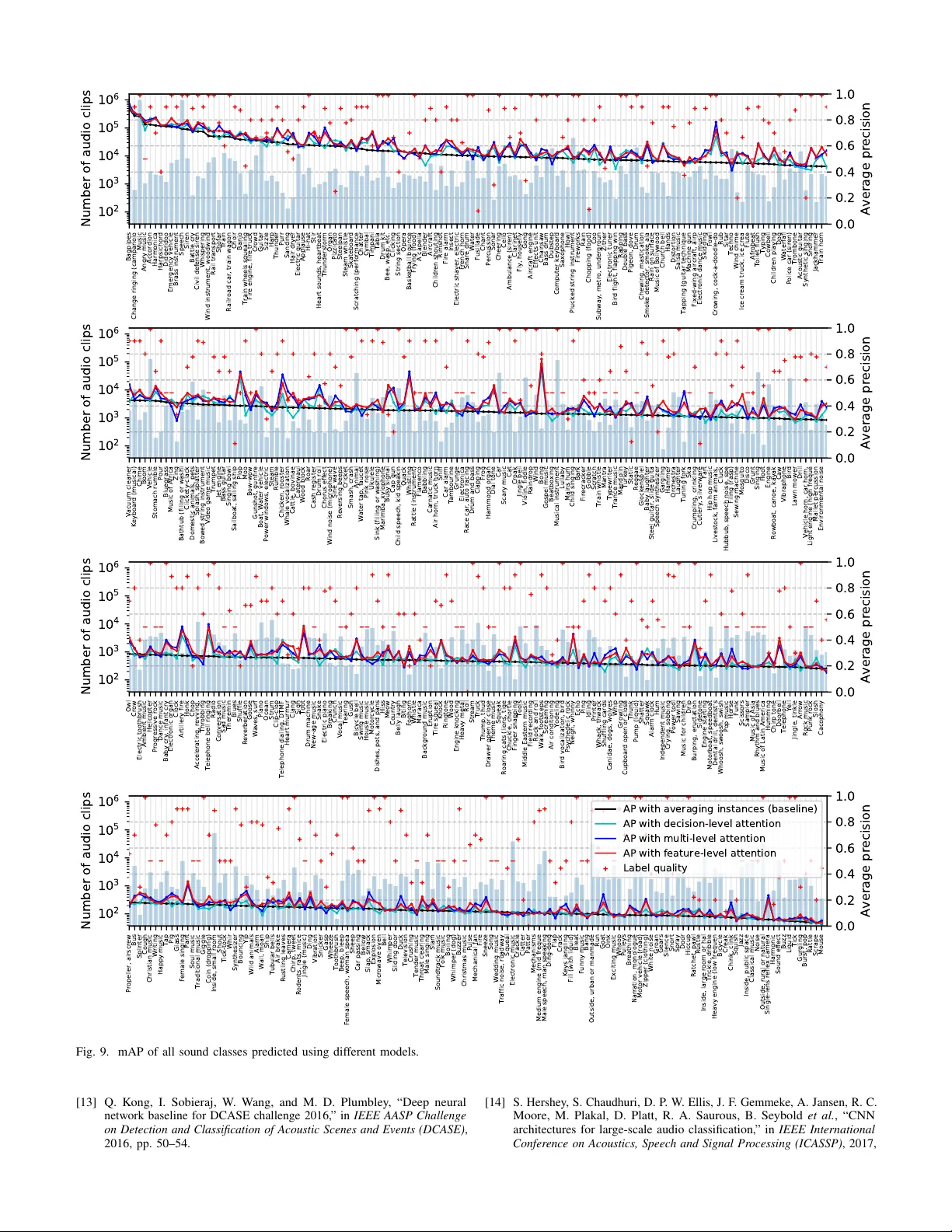
Published as a journal paper at IEEE/A CM Transactions on Audio, Speech, and Language Processing, v ol. 27, no. 11, pp. 1791-1802, Nov . 2019 W eakly Labelled AudioSet T agging with Attention Neural Networks Qiuqiang K ong, Student Member , IEEE , Changsong Y u, Y ong Xu, Member , IEEE , T urab Iqbal, W enwu W ang, Senior Member , IEEE and Mark D. Plumbley , F ellow , IEEE Abstract —A udio tagging is the task of pr edicting the pr esence or absence of sound classes within an audio clip. Previous w ork in audio tagging f ocused on relativ ely small datasets limited to recognising a small number of sound classes. W e investigate audio tagging on AudioSet, which is a dataset consisting of over 2 million audio clips and 527 classes. A udioSet is weakly labelled, in that only the presence or absence of sound classes is known for each clip, while the onset and offset times are unknown. T o address the weakly-labelled audio tagging problem, we propose attention neural networks as a way to attend the most salient parts of an audio clip. W e bridge the connection between attention neural networks and multiple instance learning (MIL) methods, and propose decision-level and feature-le vel attention neural networks for audio tagging. W e inv estigate attention neural networks modelled by different functions, depths and widths. Experiments on A udioSet show that the feature-level attention neural network achieves a state-of-the-art mean average precision (mAP) of 0.369, outperforming the best multiple in- stance learning (MIL) method of 0.317 and Google’ s deep neural network baseline of 0.314. In addition, we discover that the audio tagging perf ormance on A udioSet embedding features has a weak correlation with the number of training samples and the quality of labels of each sound class. Index T erms —A udio tagging, A udioSet, attention neural net- work, weakly labelled data, multiple instance learning . I . I N T R O D U C T I O N Audio tagging is the task of predicting the tags of an audio clip. Audio tagging is a multi-class tagging problem to predict zero, one or multiple tags for an audio clip. As a specific task of audio tagging, audio scene classification often inv olves the prediction of only one label in an audio clip, i.e. the type of environment in which the sound is present. In this paper , we focus on audio tagging. Audio tagging has many applications such as music tagging [1] and information retriev al Manuscript received March 13, 2019; revised June 18, 2019; accepted July 11, 2019. Date of publication July 26, 2019; date of current version August 21, 2019. This work was supported in part by the EPSRC Grant EP/N014111/1 “Making Sense of Sounds”, in part by the Research Scholarship from the China Scholarship Council 201406150082, and in part by a studentship (Reference: 1976218) from the EPSRC Doctoral Training Partnership under Grant EP/N509772/1. The associate editor coordinating the revie w of this manuscript and approving it for publication was Dr. Alexey Ozerov . ( Qiuqiang K ong is first author .) (Corresponding author: Y ong Xu.) Q. K ong, T . Iqbal, and M. D. Plumble y are with the Centre for V ision, Speech and Signal Processing, University of Surrey , Guildford GU2 7XH, U.K. (e-mail: q.kong@surrey .ac.uk; t.iqbal@surrey .ac.uk; m.plumbley@surrey .ac.uk). Y . Xu is with the T encent AI Lab, Bellevue, W A 98004 USA (e-mail: lucayongxu@tencent.com). W . W ang is with the Centre for V ision, Speech and Signal Processing, Univ ersity of Surrey , Guildford GU2 7XH, U.K., and also with Qingdao Univ ersity of Science and T echnology , Qingdao 266071, China (e-mail: w .wang@surrey .ac.uk). Digital Object Identifier 10.1109/T ASLP .2019.2930913 [2]. An example of audio tagging that has attracted significant attention in recent years is the classification of environmental sounds, that is, predicting the scenes where they are recorded. For instance, the Detection and Classification of Acoustic Scenes and Events (DCASE) challenges [3]–[6] consist of tasks from a variety of domains, such as DCASE 2018 T ask 1 classification of outdoor sounds, DCASE 2017 T ask4 tagging of street sounds and DCASE 2016 T ask4 tagging of domestic sounds. These challenges provide labelled datasets, so it is possible to use supervised learning algorithms for audio tagging. Ho wev er , many audio tagging datasets are relatively small [3]– [6], ranging from hundreds to thousands of training samples, while modern machine learning methods such as deep learning [7, 8] often benefit greatly from larger dataset for training. In 2017, a large-scale dataset called AudioSet [9] was released by Google. AudioSet consists of audio clips extracted from Y ouTube videos, and is the first dataset that achiev es a similar scale to the well-known ImageNet [10] dataset in computer vision. The current v ersion (v1) of AudioSet consists of 2,084,320 audio clips organised into a hierarchical ontology with 527 predefined sound classes in total. Each audio clip in AudioSet is approximately 10 seconds in length, leading to 5800 hours of audio in total. AudioSet provides an opportunity for researchers to in vestigate a large and broad v ariety of sounds instead of being limited to small datasets with limited sound classes. One challenge of AudioSet tagging is that AudioSet is a weakly-labelled dataset (WLD) [11, 12]. That is, for each audio clip in the dataset, only the presence or the absence of sound classes is indicated, while the onset and offset times are unknown. In pre vious work in audio tagging, an audio clip is usually split into segments and each segment is assigned with the label of the audio clip [13]. Howe ver , as the onset and offset of sound events are unknown so such label assignment can be incorrect. For example, a transient sound e vent may only appear a short time in a long audio recording. The duration of sound ev ents can be very different and there is no prior kno wledge of their duration. Different from ImageNet [10] for image classification where objects are usually centered and ha v e similar scale, in AudioSet the duration of sound e vents may v ary a lot. T o illustrate, Fig. 1 from top to bottom shows: the log mel spectrogram of a 10-second audio clip 1 ; AudioSet bottleneck features [9] extracted by a pre-trained VGGish con v olutional network followed by a principal component analysis (PCA); weak labels of the audio including “music”, “chuckle”, “snicker” 1 https://www .youtube.com/embed/Wxa36SSZx8o?start=70&end=80 1 2 VGG + PCA . . . . . . AudioSet Log mel spectrogram Chuckle, Snicker Music Speech VGG + PCA . . . AudioSet bottleneck featur es Weak l abels Music, Chuckle, Snicker , Speech Fig. 1. From top to bottom: Log mel spectrogram of a 10-second audio clip; AudioSet bottleneck features extracted by a pre-trained VGGish conv olutional neural network followed by a principle component analysis (PCA) [14]; W eak labels of the audio clip. There are no onset and offset times of the sound classes. and “speech’. In contrast to WLD, strongly labelled data (SLD) refers to the data labelled with both the presence of sound classes as well as their onset and offset times. For example, the sound e vent detection tasks in DCASE challenge 2013, 2016, 2017 [3, 5, 6] provide SLD. Howe ver , labelling onset and offset times of sound ev ents is time-consuming, so these strongly labelled datasets are usually limited to a relativ ely small size [3, 5, 6], which may limit the performance of deep neural networks that require large data to train a good model. In this paper , we train an audio tagging system on the large- scale weakly labelled AudioSet. W e bridge our previously proposed attention neural networks [15, 16] with multiple instance learning (MIL) [17] and propose decision-level and feature-lev el attention neural networks for audio tagging. The contributions of this paper include the following: • Decision-le vel and feature-lev el attention neural networks are proposed for audio tagging; • Attention neural netw orks modelled by dif ferent functions, widths and depth are in vestigated; • The impact of the number of training samples per class on the audio tagging performance is studied; • The impact of the quality of labels on the audio tagging performance is studied. This paper is organised as follows. Section II introduces audio tagging with weakly labelled data. Section III introduces our previously proposed attention neural networks [15, 16]. Section IV introduces multiple instance learning. Section V revie ws attention neural networks under the MIL framework and proposes decision-lev el and feature-lev el attention mod- els. Section VI shows the experimental results. Section VII concludes and forecasts future work. I I . A U D I O T AG G I N G W I T H W E A K L Y L A B E L L E D DA TA Audio tagging has attracted much research interests in recent years. For example, the tagging of the CHiME Home dataset [18], the UrbanSound dataset [19] and datasets from the Detection and Classification of Acoustic Scenes and Events (DCASE) challenges in 2013 [20], 2016 [21], 2017 [6] and 2018 [22]. The DCASE 2018 Challenge includes acoustic scene classification [22], general purpose audio tagging [23] and bird audio detection [24] tasks. Mel frequency cepstral coefficients (MFCC) [25]–[27] hav e been widely used as features to build audio tagging systems. Other features used for audio tagging include pitch features [26] and I-vectors [27]. Classifiers include such as Gaussian mixture models (GMMs) [28] and support vector machines [29]. Recently , neural networks hav e been used for audio tagging with mel spectrograms as input features. A v ariety of neural network methods including fully-connected neural networks [13], con volutional neural networks (CNNs) [14, 30, 31] and con v olutional recurrent neural networks (CRNNs) [32, 33] have been explored for audio tagging. For sound localization, an identify , locate and separate model [34] was proposed for audio-visual object extraction in large video collections using weak supervision. A WLD consists of a set of bags , where each bag is a collection of instances. For a particular sound class, a positi ve bag contains at least one positive instance, while a neg ativ e bag contains no positiv e instances. W e denote the n -th bag in the dataset as B n = { x n 1 , ..., x nT n } , where T n is the number of instances in the bag. An instance x nt ∈ R M in the bag has a dimension of M . A WLD can be denoted as D = { B n , y n } N n =1 , where y n ∈ { 0 , 1 } K denotes the tags of bag B n , and K and N are the number of classes and training samples, respectiv ely . In WLD, each bag B n has associated tags but we do not know the tags of individual instances x nt within the bag [35]. For example, in the AudioSet dataset, a bag consists of instances that are bottleneck features obtained by inputting a logmel to a pre-trained VGGish con volutional neural network. In the following sections, we omit the training example index n and the time index t to simplify notation. Pre vious audio tagging systems using WLD have been based on segment based methods. Each segment is called an instance and are assigned the tags inherited from the audio clip. During training, instance-lev el classifiers are trained on individual instances. During inference, bag-lev el predictions are obtained by aggregating the instance-lev el predictions [13]. Recently , con v olutional neural networks hav e been applied to audio tagging [32], where the log spectrogram of an audio clip is used as input to a CNN classifier without predicting the individual instances explicitly . Attention neural networks have been proposed for AudioSet tagging in [15, 16]. Later , a clip- lev el and segment-le vel model with attention supervision was proposed in [36]. I I I . A U D I O T AG G I N G W I T H A T T E N T I O N N E U R A L N E T W O R K S A. Segment based methods R3: In segment based methods, an audio clip is split into segments and each segment is assigned the tags inherited from the audio clip. In MIL, each segment is called an instance. An instance-le vel classifier f is trained on the individual instances: f : x 7→ f ( x ) , where f ( x ) ∈ [0 , 1] K predicts the presence probabilities of sound classes. The function f depends on a set of learnable parameters that can be optimised using gradient descent methods with the loss function l ( f ( x ) , y ) = d ( f ( x ) , y ) , (1) 3 where y ∈ { 0 , 1 } K are the tags of the instance x and d ( · , · ) is a loss function. For instance, it could be binary cross-entropy for multi-class tagging, given by d ( f ( x ) , y ) = − K X k =1 [ y k log f ( x ) k +(1 − y k ) log (1 − f ( x ) k ] . (2) In inference, the prediction of a bag is obtained by aggregating the predictions of individual instances in the bag such as by majority voting [13]. The segment based model has been applied to many tasks such as information retriev al [37] due to its simplicity and efficiency . Howe ver , the assumption that all instances inherit the tags of a bag is incorrect. For example, some sound ev ents may only occur for a short time in an audio clip. B. Attention neural networks Attention neural networks were first proposed for natural language processing [38, 39], where the words in a sentence are attended differently for machine translation. Attention neural networks are designed to attend to important words and ignore irrelev ant words. Attention models hav e also been applied to computer vision, such as image captioning [40] and information retrie val [41]. W e proposed attention neural networks for audio tagging and sound event detection with WLD in [15, 33]: these were ranked first in the DCASE 2017 T ask 4 challenge [33]. In a similar way to the segment based model, attention neural networks build an instance-lev el classifier f ( x ) for individual instances x . In contrast to the segment based model, attention neural networks do not assume that instances in a bag hav e the same tags as the bag. As a result, there is no instance-le vel ground truth for supervised learning using (1). T o solve this problem, we aggregate the instance-lev el predictions f ( x ) to a bag-level prediction F ( B ) giv en by F ( B ) k = X x ∈ B p ( x ) k f ( x ) k , (3) where p ( x ) k is a weight of f ( x ) k that we refer to as an attention function . The attention function p ( x ) k should satisfy X x ∈ B p ( x ) k = 1 , (4) so that the bag-lev el prediction can be seen as a weighted sum of the instance-level predictions. Both the attention function p ( x ) and the instance-lev el classifier f ( x ) depend on a set of learnable parameters. The attention function p ( x ) k controls ho w much a prediction f ( x ) k should be attended. Large p ( x ) k indicates that f ( x ) k should be attended, while small p ( x ) k indicates that f ( x ) k should be ignored. T o satisfy (4), the attention function p ( x ) k can be modelled as p ( x ) k = v ( x ) k / X x ∈ B v ( x ) k , (5) where v ( · ) can be any non-ne gati v e function to ensure that p ( · ) is a probability . An extension of the attention neural network in (3) is the multi-lev el attention model [16], where multiple attention modules are applied to utilise the hierarchical information of neural networks: F ( B ) = g ( F 1 ( B ) , ..., F L ( B )) , (6) where F l ( B ) is the output of the l -th attention module and L is the number of attention modules. Each F l ( B ) can be modeled by (3). Then a mapping g is used to map from the predictions of L attention modules to the final prediction of a bag. The multi-lev el attention neural network has achiev ed state-of-the-art performance in AudioSet tagging. In the next section, we show that the attention neural networks explored above can be categorised into an MIL framew ork. I V . M U LT I P L E I N S TA N C E L E A R N I N G Multiple instance learning (MIL) [17, 42] is a type of supervised learning method. Instead of receiving a set of labelled instances, the learner receiv es a set of labelled bags. MIL methods have many applications. For example, in [42], MIL is used to predict whether new molecules are qualified to make some new drug, where molecules may hav e many alternativ e low-ener gy states, but only one, or some of them, are qualified to make a drug. Inspired by the MIL methods, a sound ev ent detection system trained on WLD [11] was proposed. General MIL methods include the expectation- maximization div ersity density (EM-DD) method [43], support vector machine (SVM) methods [44] and neural network MIL methods [45, 46]. In [47], sev eral MIL pooling methods were in v estigated in audio tagging. Attention-based deep multiple instance learning is proposed in [48]. In [35], MIL methods are grouped into three categories: the instance space (IS) methods, where the discriminativ e information is considered to lie at the instance-lev el; the bag space (BS) methods, where the discriminativ e information is considered to lie at the bag-level; and the embedded space (ES) methods, where each bag is mapped to a single feature vector that summarises the relev ant information about a bag. W e introduce the IS, BS and ES methods in more detail below . A. Instance space methods In IS methods, an instance-lev el classifier f : x 7→ f ( x ) is used to predict the tags of an instance x , where f ( x ) ∈ [0 , 1] K predicts the presence probabilities of sound classes. The IS methods introduce aggregation functions [35] to con vert an instance-lev el classifier f to a bag-lev el classifier F : B 7→ [0 , 1] K , given by F ( B ) = agg ( { f ( x ) } x ∈ B ) , (7) where agg ( · ) is an aggregation function. The classifier f depends on a set of learnable parameters. When the IS method is trained with (1) in which each instance inherits the tags of the bag, the IS method is equiv alent to the segment based model. On the other hand, the IS method can also be trained using the bag-level loss function: l ( F ( B ) , y ) = d ( F ( B ) , y ) , (8) 4 where y ∈ { 0 , 1 } K is the tag of the bag and d ( · , · ) is a loss function such as the binary cross-entropy in (2). T o model the aggregation function, the standard multiple instance (SMI) assumption and collective assumption (CA) are proposed in [35]. Under the SMI assumption, a bag-lev el classifier can be obtained by F ( B ) k = max x ∈ B f ( x ) k , (9) where the subscript k denotes the k -th sound class of the instance-lev el prediction f ( x ) and the bag-lev el prediction F ( B ) . Under the SMI assumption, for the k -th sound class, only one instance with the maximum prediction probability is chosen as a positive instance. One problem of the SMI assumption is that a positiv e bag may contain more than one positive instance. In SED, some sound classes such as “ambulance siren” may last for sev eral seconds and may occur in many instances. In contrast to the SMI assumption, with the CA assumption, all the instances in a bag contribute equally to the tags of the bag. The bag- le vel prediction can be obtained by av eraging the instance-level predictions: F ( B ) = 1 | B | X x ∈ B f ( x ) . (10) The symbol | B | denotes the number of instances in bag B . Equation (10) shows that CA is based on the assumption that all the instances in a positiv e bag are positive. B. Bag space methods Instead of building an instance-le vel classifier , the BS methods re gard a bag B as an entirety . Building a tagging model on the bags rely on a distance function D ( · , · ) : B × B 7→ R . The distance function can be, for example, the Hausdorff distance [49]: D ( B 1 , B 2 ) = min x 1 ∈ B 1 , x 2 ∈ B 2 k x 1 − x 2 k . (11) In (11), the distance between two bags is the minimum distance between the instances in bag B 1 and B 2 . Then this distance function can be plugged into a standard distance-based classifier such as a k-nearest neighbour (KNN) or a support vector machine (SVM) algorithm. The computational complexity of (11) is | B 1 || B 2 | , which is larger than the IS and the ES methods described below . C. Embedded space methods Different from the IS methods, ES methods do not clas- sify individual instances. Instead, the ES methods define an embedding mapping from a bag to an embedding vector: f emb : B 7→ h . (12) Then the tags of a bag is obtained by applying a function g on the embedding vector: F ( B ) = g ( h ) . (13) The embedding mapping f emb can be modelled in many ways. For example, by averaging the instances in a bag, as in the simple MI method in [50]: h = 1 | B | X x ∈ B x . (14) Alternativ ely , the mapping can be obtained in terms of the max-min operations on the instances [51]:        h = ( a 1 , ..., a M , b 1 , ..., b M ) , a m = max x ∈ B ( x m ) , b m = min x ∈ B ( x m ) , (15) where x m is the m -th dimension of x . Equation (15) shows that only one instance with the maximum or the minimum v alue is chosen for each dimension, while other instances hav e no contribution to the embedding vector h . The ES methods summarise a bag containing an arbitrary number of instances with a vector of fixed size. Similar methods hav e been proposed in natural language processing to summarise sentences with a variable number of words [52]. V . A T T E N T I O N N E U R A L N E T W O R K S U N D E R M I L In this section, we show that the pre viously proposed attention neural networks [15, 16] belong to MIL frameworks, especially the IS methods. W e refer to these attention neural networks as decision-lev el attention neural networks, because the prediction of a bag is obtained by aggregating the pre- dictions of instances (see (7)). W e then propose feature-lev el attention neural networks inspired by the ES methods with attention in the hidden layers. A. Decision-level attention neural networks The IS methods predict the tags of a bag by aggregating the predictions of individual instances in the bag described in (7). Section IV -A shows that con ventional IS methods are based on either the SMI assumption (see (9)) or the CA (see (10)). The problem of the SMI assumption is that only one instance in a bag is considered to be positiv e for a sound class while other instances are not considered. The SMI assumption is not appropriate for bags with more than one positiv e instance for a sound class. On the other hand, CA assumes that all instances in a positi ve bag are positiv e. CA is not appropriate for sound e vents that only last for a short time. T o address the problems of the SMI and CA methods, a decision-lev el attention neural network based on the IS methods in (7) is proposed to learn an attention function to weight the predictions of instances in a bag, so that F ( B ) k = agg ( { f ( x ) k } x ∈ B ) = X x ∈ B p ( x ) k f ( x ) k , (16) where p ( x ) is an attention function modelled by (5). W e refer to (16) as a decision-level attention neural network because the attention function p ( x ) is multiplied with the predictions of the instances f ( x ) to obtain the bag-le vel prediction. The attention function p ( x ) controls how much the prediction of an instance 5 p ( x ) k f ( x ) k p ( x ) f ( x ) p ( x ) k f ( x ) k p ( x ) f ( x ) p ( x ) k f ( x ) k f ( x ) p ( x ) x x (a) (c) x (b) Fwd Fig. 2. (a) Joint detection and classification (JDC) model; (b) Self attention neural network in [53]; (c) Proposed attention neural network [15]. The blue outlined block in (c) is called a forward (FWD) block. f ( x ) should be attended or ignored. Equation (16) can be seen as a general case of the SMI and CA assumptions. When one instance x in a bag has a v alue of p ( x ) = 1 the other instances hav e values of p ( x ) = 0 , then (16) is equiv alent to the SMI assumption in (9). When p ( x ) = 1 | B | for all instances in a bag, (16) is equiv alent to CA. Fig. 2 shows different ways to model the attention neural network in (16). F or e xample, Fig. 2(a) sho ws the joint detection and classification (JDC) model [12] with attention function p and the classifier f modelled by separate branches. Fig. 2(b) sho ws the self attention neural network [53] proposed in natural language processing. Fig. 2(c) shows the JDC improved by using shared layers for the attention function p and the classifier f before they separate in the penultimate layer [15]. In the attention neural networks, both p and f depend on a set of learnable parameters which can be optimised with gradient descent methods using the loss function in (8). F or the proposed model in Fig. 2(c), the attention function p and the classifier f share the low-le vel layers. W e denote the output of the layer before they separate as x 0 . The mapping from x to x 0 can be modelled by fully-connected layers, for example. x 0 = f FC ( x ) . (17) The classifier f can be modelled by f ( x ) = σ ( W 1 x 0 + b 1 ) , (18) where σ ( x ) = 1 / (1 + e − x ) is the sigmoid function. The attention function p can be modelled by ( v ( x 0 ) k = φ 1 ( U 1 x 0 + c 1 ) , p ( x ) k = v ( x 0 ) k / P x ∈ B v ( x 0 ) k , (19) where φ 1 can be any non-negati ve function to ensure p ( x ) k is a probability . B. F eature-le vel attention neural network The limitation of the decision-lev el attention neural networks is that the attention function p ( x ) is only applied to the prediction of the instances f ( x ) , as shown in (16). In this section, we propose to apply attention to the hidden layers of a neural network. This is inspired by the ES methods in (12), . . . . . . . . . Decision-level single att ention . . . 1 K K 1 . . . K 1 . . . J 1 . . . . . . De c i s i o n - l e v e l . . . K 1 . . . . . . K 1 . . . . . . . . . . . . . . . . . . . . . . . . . . . x 1 x 1 x T x T Fwd . . . . . . x 1 x T 1 K . . . 1 J 1 . . . 1 Fwd Fwd . . . Fwd Fwd . . . Fwd (a) (b) (c) Decision - level single att ention Decision-level single att ention Fig. 3. (a) Decision-level single attention neural network [15]; (b) Decision- lev el multiple attention neural network [16]; (c) Feature-level attention neural network (proposed). where a bag B is mapped to a fixed-size vector h before being classified. W e model (12) with attention aggregation: h j = X x ∈ B q ( x ) j u ( x ) j , (20) where both q ( x ) ∈ [0 , 1] J and u ( x ) ∈ R J hav e a dimension of J . The embedded v ector h ∈ R J summarises the information of a bag. Then the tags of a bag B can be obtained by classifying the embedding vector: F ( B ) = f ( h ) . (21) The probability q ( x ) j in (20) is the attention function of u ( x ) j and should satisfy X x ∈ B q ( x ) j = 1 . (22) W e model u ( x ) with u ( x ) = ψ ( W 2 x 0 + b 1 ) , (23) where ψ can be any linear or non-linear function to increase the representation ability of the model. The attention function q can be modelled by ( w ( x 0 ) j = φ 2 ( U 2 x 0 + c 2 ) , q ( x ) j = w ( x 0 ) j / P x ∈ B w ( x 0 ) j , (24) where w ( x ) j can be any non-negati ve function to ensure q ( x ) j is a probability . Fig. 3 shows the decision-le vel single attention [15], decision- lev el multiple attention [16] and the proposed feature-le vel attention neural network. The forward (Fwd) block in Fig. 3 is the same as the block in Fig. 2(c). The difference between the feature-lev el attention function q ( x ) and the decision-lev el attention function p ( x ) is that the dimension of q ( x ) can be any v alue, while the dimension of p ( x ) is fixed to be the number of sound classes K . Therefore, the capacity of the decision-lev el attention neural networks is limited. W ith an increase in the dimension of q ( x ) , the capacity of feature-level attention neural networks is increased. The decision-level attention function attends to the predictions of instances, while the feature-level attention function attends to the features, so it is equiv alent to feature selection. The multi-le vel attention model [16] in (6) can 6 1 2 3 4 5 6 7 8+ Number of sound events 0 200000 400000 600000 800000 Number of audio clips Fig. 4. Distribution of the number of sound classes in an audio clip. be seen as a special case of the feature-level attention model, with embedding vector h = ( F 1 ( B ) , ..., F L ( B )) . The superior performance of the multi-lev el attention model shows that the feature-lev el attention neural networks hav e the potential to perform better than the decision-level attention neural networks. C. Modeling the attention function with differ ent non-linearity W e adopt Fig. 2(c) as the backbone of our attention neural networks. The attention function p and q for the decision-lev el and feature-lev el attention neural networks are obtained via non-negati ve functions φ 1 and φ 2 , respectiv ely . The φ 1 and φ 2 appearing in the summation term of the denominator of (19) and (24) may affect the optimisation of the attention neural networks. W e inv estigate modelling φ 2 in the feature- lev el attention neural networks with different non-negati ve functions, including ReLU [54], exponential, sigmoid, softmax and network-in-network (NIN) [55]. W e omit the ev aluation of φ 1 , as the feature-le vel attention neural networks outperform the decision-lev el attention neural networks. The ReLU function is defined as [54] φ ( z ) = max ( z , 0) . (25) The exponential function is defined as φ ( z ) = e z . (26) The sigmoid function is defined as φ ( z ) = 1 1 + e − z . (27) For a vector z , the softmax function is defined as φ ( z j ) = e z j P k e z k . (28) The network-in-network function [55] is defined as φ ( z ) = σ ( H 2 ψ ( H 1 z + d 1 ) + d 2 ) , (29) where H 1 , H 2 are transformation matrices, d 1 and d 2 are biases, ψ is ReLU nonlinearity and σ is the sigmoid function. VGGis h CNN AudioSet 2 million clips 527 classes Y ouT ube 100M 20 billion clips 3087 classes Log mel spectrogr am AudioSet bottleneck feat ures Log mel spectrogr am Inference Fig. 5. A VGGish CNN model is trained on the Y ouTube 100M dataset. Audio clips from AudioSet are given as input to the trained V GGish CNN to extract the bottleneck features, which are released by AudioSet. V I . E X P E R I M E N T S A. Dataset W e ev aluate the proposed attention neural networks on AudioSet [9], which consists of 2,084,320 10-second audio clips extracted from Y ouT ube video with a hierarchical ontology of 527 classes in the released version (v1). W e released both Keras and PyT orch implementations of our code online 2 . AudioSet consists of a variety of sounds. AudioSet is multi-labelled, such that each audio clip may contain more than one sound class. Fig. 4 shows the statistics of the number of sound classes in the audio clips. All audio clips contain at least one label. Out of ov er 2,084,320 audio clips, there are 896,045 audio clips containing one sound class, followed by around 684,166 audio clips containing two sound classes. Only 4,661 audio clips hav e more than 7 labels. Instead of providing raw audio wav eforms, AudioSet pro- vides bottleneck features of audio clips. The bottleneck features are extracted from the bottleneck layer of a VGGish CNN, pre-trained on 70 million audio clips from the Y ouT ube100M dataset [14]. The VGGish CNN consists of 6 conv olutional layers with kernel size of 3 × 3 and 2 fully layers. T o begin with, the 70 million training audio clips are segmented to non- ov erlapping 960 ms segments. Each segment inherits all tags of its parent video. Then short-time Fourier transform (STFT) is applied on each 960 ms segment with a window size of 25 ms and a hop size of 10 ms to obtain a spectrogram. Then a mel filter bank with 64 frequency bins is applied on the spectrograms followed by a logarithmic operation to obtain log mel spectrograms. Each log mel spectrogram of a segment has a shape of 96 × 64 , representing the time steps and the number of mel frequency bins. A VGGish CNN is trained on these log mel spectrograms with the 3087 most frequent labels. After training, the VGGish CNN is used as a feature extractor . By inputting an audio clip to the VGGish CNN, the outputs of the bottleneck layer are used as bottleneck features of the audio clip. The framework of AudioSet feature extraction is shown in Fig. 5. B. Evaluation criterion W e first introduce basic statistics [56]: true positiv e (TP), where both the reference and the system prediction indicate an event to be activ e; false negati ve (FN), where the reference indicates an ev ent is acti ve but the system prediction indicates 2 https://github .com/qiuqiangkong/audioset_classification 7 Music Speech Vehicle Musical instrument Inside, small room Guitar Plucked string instr Singing Car Animal Electronic music Outside, rural or Outside, urban or Violin, fiddle Inside, large room Bird Drum Domestic animals, Dubstep Male speech, man spe Techno Percussion Engine Narration, monologue Drum kit Acoustic guitar Strum Dog Boat, Water vehicle Train Electric guitar 1 0 2 1 0 3 1 0 4 1 0 5 1 0 6 Number of audio clips Power windows, elect Crack Stomach rumble Whale vocalization Chirp tone Bicycle bell Foghorn Wail, moan Bouncing Chopping (food) Sniff Pulse Zing Tuning fork Sidetone Squeak Sanding Cupboard open or clo Wheeze Squeal Dental drill, dentis Crushing Hoot Finger snapping Squawk Splinter Pulleys Creak Gargling Toothbrush 0.0 0.2 0.4 0.6 0.8 1.0 Average precision Full training data samples Bal. training data samples AP with averaging instances (baseline) Fig. 6. AudioSet statistics. Upper bars: the number of audio clips of a specific sound class sorted in descending order plotted in log scale with respect to the sound classes. Red stems: average precision (AP) of sound classes with the feature-le vel attention model. T ABLE I B A S E L I N E R E S U LTS O F S E G M E N T B A S E D M E T H O D , I S A N D E S M E T H O D S mAP A UC d-prime Random guess 0.005 0.500 0.000 Google baseline [9] 0.314 0.959 2.452 Segment based [13] 0.293 0.960 2.483 (IS) SMI assumption [11] 0.292 0.960 2.471 (IS) Collectiv e assumption 0.300 0.964 2.536 (ES) A verage instances [50] 0.317 0.963 2.529 (ES) Max instance 0.284 0.958 2.443 (ES) Min instance 0.281 0.956 2.413 (ES) Max-min instance [51] 0.306 0.962 2.505 an ev ent is inactive; false positive (FP), where the system prediction indicates an ev ent is acti ve b ut the reference indicates it is inactiv e; true negati ve (TN), where both the reference and the system prediction indicate an ev ent is inactive. Precision (P) and recall (R) are defined as in [56]: P = TP TP + FP , R = TP TP + FN . (30) In addition, the false positiv e rate is defined as [56] FPR = FP FP + TN . (31) Follo wing [9], we adopt mean av erage precision (mAP), area under the curve (A UC) and d-prime as e valuation metrics. A verage precision (AP) [9] is defined as the area under the recall-precision curve of a specific class. The mean average precision (mAP) is the a verage v alue of AP ov er all classes. As AP is re gardless of TN, A UC is used as a complementary metric. A UC is the area under the receiver operating characteristic (R OC) created by plotting the recall against the false positiv e rate (FPR) at various threshold settings for a specific class. W e use mA UC to denote the av erage value of A UC over all classes. D-prime is a statistic used in signal detection theory that provides separation between signal and noise distributions. D-prime is obtained via a transformation of A UC and has a better dynamic range than A UC when A UC is larger than 0.9. A T ABLE II R E S U LT S O F E S AVE R AG E I N S T A N C E S M E T H O D W I T H D I FF E R E N T BA L A N C I N G S T R ATE G Y . mAP A UC d-prime Balanced data 0.274 0.949 2.316 Full data (no bal. training) 0.268 0.950 2.331 Full data (bal. training) 0.317 0.963 2.529 higher mAP , A UC and d-prime indicates a better performance. D-prime can be calculated by [9]: d-prime = √ 2 F − 1 x ( A UC ) , (32) where F − 1 x is an inv erse of the cumulative distribution function defined by F x ( x ) = Z x −∞ 1 √ 2 π e − ( x − µ ) 2 2 dx. (8) C. Baseline system W e build baseline systems with segment based method, IS and ES models without the attention mechanism described in Section III-A , IV -A and IV -C , respectively . In the segment based model, a classifier is trained on individual instances, where each instance inherits the tags of a bag. A three-layer fully-connected neural network with 1024 hidden units and ReLU [54] non-linearity is applied. Dropout [57] with a rate of 0.5 is used to pre v ent o verfitting. The loss function for training is giv en in (1). In inference, the prediction is obtained by av eraging the prediction of indi vidual instances. The IS models hav e the same structure as the segment based model. Dif ferent from the segment based model, the instance-lev el predictions by the IS models are aggregated to a bag-lev el prediction by either the SMI assumption in (9) or CA in (10). The loss function is calculated from (8). The ES method aggregates the instances of a bag to an embedded vector before tagging. The embedding function can be the averaging mapping in (14) or max-min vector mapping in (15). Then the embedded vector is input to a neural network in the same way as the segment based model. The loss function is calculated from (8). W e 8 adopt the Adam optimiser [58] with a learning rate of 0.001 in training. The mini-batch size is set to 500. The networks are trained for a total number of 50,000 iterations. W e average the predictions of 9 models from 10,000 to 50,000 iterations as the final prediction to ensemble and stabilise the result, which can reduce the prediction randomness caused by the model. T able I sho ws the tagging result of segment based method, IS and ES baseline methods. The first row sho ws that the random guess achieves an mAP of 0.005, an A UC of 0.500 and a d-prime of 0. The segment based model achiev es an mAP of 0.293, slightly better than the IS methods with the CA and SMI assumption, with mAP of 0.300 and 0.292, respectiv ely . The sixth to the ninth rows show that both the ES methods with av eraging and the max-min instances perform better than the segment based model and IS methods. A veraging the instances performs the best in the ES methods with an mAP of 0.317, an A UC of 0.963 and a d-prime of 2.529. D. Data balancing AudioSet is highly imbalanced, as some sound classes such as speech and music are more frequent than others. The upper bars in Fig. 6 show the number of audio clips per class sorted in descending order (in log scale). The data has a long tail distribution. Music and speech appear in almost 1 million audio clips while some sounds such as gargling and toothbrush only appear in hundreds of audio clips. AudioSet provides a balanced subset consisting of 22,160 audio clips. The lower bars in Fig. 6 show the number of audio clips per class of the balanced subset. When training a neural network, data is loaded in mini batches. W e found that without a balancing strategy , the classes with fewer samples are less likely to be selected in training. Sev eral balancing strategies have been inv estigated in image classification such as balancing the frequent and infrequent classes [59]. In this paper , we follow the mini-batch balancing strategy [15] for AudioSet tagging, where each mini-batch is balanced to have approximately the same number of samples in training the neural network. W e first inv estigate the performance of training on the balanced subset only and training on the full data. W e adopt the best baseline model; that is, the ES average instances model in Section IV -C . T able II shows that the model trained with only the balanced subset achiev es an mAP of 0.274. The model trained with the full dataset without balancing achieves an mAP of 0.268. The model trained with the balancing strategy achiev es an mAP of 0.317. Fig. 7 shows the class-wise AP . The dashed and solid curves show the training and testing AP , respecti vely . In addition, Fig. 7 sho ws that the AP is not al ways positi ve related to the number of training samples. For example, when using full data for training, “bagpipes” has 1,715 audio clips but achiev es an mAP of 0.884, while “outside” has 34,117 audio clips but only achieves an AP of 0.093. W e disco ver that for a majority of sound classes, the improvement of AP is small compared when using the full dataset rather than the balanced subset. For example, there are 60 and 1,715 “bagpipes” audio clips in the balanced subset and the full dataset, respectively . Their APs are 0.873 and 0.884, respectiv ely , indicating that collecting more data for “bagpipes” does not substantially improv e its tagging result. T ABLE III C O R R E L ATI O N O F M A P W I T H T R A I N I N G S A M P L E S A N D L A B E L S Q UA L I T Y O F S O U N D C L A S S E S . PCC p-value T raining examples 0.169 9.35 × 10 − 5 Labels quality 0.230 7 × 10 − 7 T o inv estigate how AP is related to the number of training samples, we calculate their Pearson correlation efficient (PCC) 3 . PCC is a number between -1 and +1. The PCC of -1, 0, +1 indicate negati v e correlation, no correlation and positive correlation, respectiv ely . The null hypothesis is that the correlation of the pair of random variables is 0. The p-value indicates the confidence when the null hypothesis is satisfied. If the p-value is lower than the con ventional 0.05 the PCC is called statistically significant. T able III shows that AP and the number of training samples hav e a correlation with a PCC of 0.169 and the p-value is 9 . 35 × 10 − 5 , indicating that AP is only weakly positiv ely related with the number of training samples. E. Noisy labels AudioSet contains noisy tags [9]. That is, some tags for training may be incorrect. There are three major reasons leading to the noisy tags in AudioSet shown in [9]: 1) confusing labels, where some sound classes are easily confused with others; 2) human error, where the labeling procedure may be flawed; 3) faint/non-salient sounds, where some sound are faint to recognise in an audio clip. Sound classes with a high label confidence include “christmas music” and “accordion”. Sound classes with a low label confidence include “boiling” and “bicycle”. T o in vestigate how accurate are the ground truth tags, The authors of AudioSet conducted an internal quality assessment task where experts checked 10 random segments for most of the classes. The quality is a value between 0 and 1 measured by the percentage of correctly labelled audio clips verified by human. The quality of labels is shown in Fig. 7 with red plus symbols. Hyphen symbols are plotted for the classes that have not been ev aluated. W e discover that AP is not always correlated positively with the quality of labels. For example, our model achiev es an AP of 0.754 in recognizing “harpsichord”, while the human label quality is 0.4. On the other hand, humans achiev e a label quality of 1.0 in “hiccup”, but the AP of our model is 0.076. T able III sho ws that AP and the quality of labels have a weak PCC of 0.230, indicating AP is only weakly correlated with the quality of labels. F . Attention neural networks W e e v aluate the decision-lev el and the feature-le vel attention neural networks in this subsection. W e adopt the architecture in Fig. 2(c) as our model. The output x 0 of the layer before the attention function is obtained by (17). Then the decision-le vel 3 Giv en a pair of random variables X and Y , the PCC is calculated as cov(X, Y) σ X σ Y , where cov ( · , · ) is the covariance of two variables and σ is the standard deviation of the random variables. 9 Bagpipes Change ringing (camp Music Angry music Accordion Harmonica Harpsichord Didgeridoo Emergency vehicle Brass instrument Speech Siren Battle cry Civil defense siren Whispering Wind instrument, woo Rail transport Shofar Train Railroad car, train Choir Banjo Train wheels squeali Fire engine, fire Crowd Guitar Sizzle Harp Thunder Purr Sanding 1 0 2 1 0 3 1 0 4 1 0 5 1 0 6 Number of audio clips Silence Snort Spray Door Hiccup Ratchet, pawl Rustle Inside, large room Trickle, dribble Heavy engine (low Bicycle Creak Chink, clink Squish Jazz Inside, public space Classical music Noise Outside, rural or Single-lens reflex Harmonic Sound effect Buzz Liquid Tick Gurgling Burst, pop Rattle Scrape Mouse 0.0 0.2 0.4 0.6 0.8 1.0 Average precision Tr. AP (bal. data, w/o bal. strategy) Te. AP (bal. data, w/o bal. strategy) Tr. AP (full data, w/o bal. strategy) Te. AP (full data, w/o bal. strategy) Tr. AP (full data, with bal. strategy) Te. AP (full data, with bal. strategy) Full training data samples Bal. training data samples Label quality Fig. 7. Class-wise AP of sound events using the IS average instances model trained with different balancing strategy . Abbreviations: Tr .: Training; T e.: T esting; bal.: training with balanced subset; full: trained with full dataset; w/o: without mini-batch data balancing; w .: with mini-batch data balancing. Bagpipes Change ringing (camp Music Angry music Accordion Harmonica Harpsichord Didgeridoo Emergency vehicle Brass instrument Speech Siren Battle cry Civil defense siren Whispering Wind instrument, woo Rail transport Shofar Train Railroad car, train Choir Banjo Train wheels squeali Fire engine, fire Crowd Guitar Sizzle Harp Thunder Purr Sanding 1 0 2 1 0 3 1 0 4 1 0 5 1 0 6 Number of audio clips Silence Snort Spray Door Hiccup Ratchet, pawl Rustle Inside, large room Trickle, dribble Heavy engine (low Bicycle Creak Chink, clink Squish Jazz Inside, public space Classical music Noise Outside, rural or Single-lens reflex Harmonic Sound effect Buzz Liquid Tick Gurgling Burst, pop Rattle Scrape Mouse 0.0 0.2 0.4 0.6 0.8 1.0 Average precision AP with averaging instances (baseline) AP with decision-level attention AP with multi-level attention AP with feature-level attention Full training data samples Bal. training data samples Label quality Fig. 8. Class-wise AP of sound ev ents predicted using different models. and feature-le vel attention neural networks are modelled by (16) and (20), respectiv ely . The first row of T able IV shows that the ES method with averaged instances achiev es an mAP of 0.317. The second and third rows sho w that the JDC model in Fig. 2(a) and the self-attention model in Fig. 2(b) achie ve an mAP of 0.337 and 0.324, respecti vely . The fourth and fifth ro w show that the decision-lev el attention neural network achiev es an mAP of 0.337. The decision-lev el multiple attention neural network further improves this result to an mAP of 0.357. The results of the feature-lev el attention neural networks are shown in the bottom block of T able IV. The ES methods with av erage and maximum aggregation achiev e an mAP of 0.298 and 0.343, respectiv ely . The feature-lev el attention neural network achiev es an mAP of 0.361, an mA UC of 0.969 and a d-prime of 2.641, outperforming the other models. One explanation is that the feature-lev el attention neural network can attend to or ignore the features in the feature space which further improves the capacity of the decision-le vel attention neural network. Fig. 8 sho ws the class-wise performance of the attention neural networks. The feature-lev el attention neural network outperforms the decision-lev el attention neural network and the ES method with av eraged instances in a majority of sound classes. The results of all 527 sound classes are shown in Fig. 9. T ABLE IV R E S U LT S O F D E C I S I O N - L E V E L ATT E N T I O N M O D E L A N D F E ATU R E - L E V E L A T T E N T I O N M O D E L mAP A UC d-prime A verage instances [50] 0.317 0.963 2.529 JDC [12] 0.337 0.963 2.526 Self attention [48] 0.324 0.962 2.506 Decision-lev el single-attention [15] 0.337 0.968 2.612 Decision-lev el multi-attention [16] 0.357 0.968 2.621 Feature-lev el avg. pooling 0.298 0.960 2.475 Feature-lev el max pooling 0.343 0.966 2.589 Feature-lev el attention 0.361 0.969 2.641 G. Modeling attention function with differ ent functions As described in Section V -C , we model the attention function q of the feature-lev el attention neural network via a non- negati ve function φ 2 . The choice of the non-negati ve function may affect the optimisation and result of the attention neural network. T able V shows that the exponential, sigmoid, softmax and NIN functions achie ve a similar mAP of approximately 0.360. Modeling φ ( · ) with ReLU is worse than with other non-linear functions.. 10 T ABLE V R E S U LT S O F M O D E L I N G T H E N O N - N E G ATI V E φ 2 W I T H D I FF E R E N T N O N - N E G A T I V E F U N C T I O N S . mAP A UC d-prime ReLU att 0.308 0.963 2.520 Exp. att 0.358 0.969 2.631 Sigmoid att 0.361 0.969 2.641 Softmax att 0.360 0.969 2.636 NIN 0.359 0.969 2.637 T ABLE VI R E S U LT S O F M O D E L I N G T H E AT T E N T I O N N E U R A L N E T W O R K W I T H D I FF E R E N T L A Y E R D E P T H S . Depth mAP A UC d-prime 0 0.328 0.963 2.522 1 0.356 0.967 2.605 2 0.358 0.968 2.620 3 0.361 0.969 2.641 4 0.356 0.969 2.637 6 0.348 0.968 2.619 8 0.339 0.967 2.595 10 0.331 0.966 2.579 T ABLE VII R E S U LT S O F M O D E L I N G T H E AT T E N T I O N N E U R A L N E T W O R K W I T H D I FF E R E N T N U M B E R O F H I D D E N U N I T S . Hidden units mAP A UC d-prime 256 0.305 0.962 2.512 512 0.339 0.967 2.599 1024 0.361 0.969 2.641 2048 0.369 0.969 2.640 4096 0.369 0.968 2.619 H. Attention neural networks with differ ent embedding depth and width As shown in (17), our attention neural networks map the instances x to x 0 through sev eral non-linear embedding layers to increase the representation ability of the instances. W e model f FC using the feature-level attention neural network with fully- connected layers with dif ferent depths. T able VI sho ws that the mAP increases from 0 layers and reaches a peak of 0.361 at 3 layers. More hidden layers do not increase the mAP . The reason might be that the AudioSet bottleneck features obtained by a VGGish CNN trained on Y ouT ube100M ha ve good separability . Therefore, there is no need to apply very deep neural networks on the AudioSet bottleneck features. On the other hand, the Y ouTube100M data may have a different distribution from AudioSet. As a result, the embedding mapping f FC can be used as domain adaption. Based on the network f FC modelled with three layers in the feature-le vel attention neural network, we in vestigate the width of f FC . T able VII sho ws that feature-level attention model with 2048 hidden units in each hidden layer achiev es an mAP of 0.369, an mA UC of 0.969 and a d-prime of 2.641 is achieved, outperforming the models with 256, 512, 1024 and 4096 hidden units in each layer . On the other hand, with 4096 hidden units, the model tends to overfit, and does not outperform the model with 2048 hidden units. V I I . C O N C L U S I O N W e hav e presented a decision-lev el and a feature-level attention neural network for AudioSet tagging. W e developed the connection between multiple instance learning and attention neural networks. W e inv estigated the class-wise performance of all the 527 sound classes in AudioSet and discov ered that the AudioSet tagging performance on AudioSet embedding features is only weakly correlated with the number of training examples and quality of labels, with Pearson correlation coefficients of 0.169 and 0.230, respectiv ely . In addition, we in v estigated modelling the attention neural networks with different attention functions, depths and widths. Our proposed feature-lev el attention neural network achiev es a state-of-the- art mean av erage precision (mAP) of 0.369 compared to the best MIL method of 0.317 and the decision-le vel attention neural network of 0.337. In the future, we will explore weakly labelled sound event detection on AudioSet with attention neural networks. A C K N O W L E D G M E N T The authors would like to thank all anonymous revie wers for their suggestions to improve this paper . R E F E R E N C E S [1] Z. Fu, G. Lu, K. M. T ing, and D. Zhang, “ A surve y of audio-based music classification and annotation, ” IEEE Tr ansactions on Multimedia , vol. 13, pp. 303–319, 2011. [2] R. T ypke, F . Wiering, and R. C. V eltkamp, “ A survey of music information retriev al systems, ” in International Confer ence on Music Information Retrieval , 2005, pp. 153–160. [3] D. Giannoulis, E. Benetos, D. Stowell, M. Rossignol, M. Lagrange, and M. D. Plumbley , “Detection and classification of acoustic scenes and ev ents: An IEEE AASP challenge, ” in IEEE W orkshop on Applications of Signal Pr ocessing to Audio and Acoustics (W ASP AA) , 2013. [4] D. Stowell, D. Giannoulis, E. Benetos, M. Lagrange, and M. D. Plumbley , “Detection and classification of acoustic scenes and e vents, ” IEEE T ransactions on Multimedia , vol. 17, no. 10, pp. 1733–1746, 2015. [5] A. Mesaros, T . Heittola, E. Benetos, P . Foster, M. Lagrange, T . V irtanen, and M. D. Plumbley , “Detection and classification of acoustic scenes and ev ents: Outcome of the DCASE 2016 challenge, ” IEEE/A CM T ransactions on Audio, Speech, and Language Processing , vol. 26, no. 2, pp. 379–393, 2018. [6] A. Mesaros, T . Heittola, A. Diment, B. Elizalde, A. Shah, E. V incent, B. Raj, and T . V irtanen, “DCASE 2017 challenge setup: T asks, datasets and baseline system, ” in DCASE W orkshop on Detection and Classifica- tion of Acoustic Scenes and Events (DCASE) , 2017, pp. 85–92. [7] Y . LeCun, Y . Bengio, and G. Hinton, “Deep learning, ” Natur e , vol. 521, no. 7553, pp. 436–444, 2015. [8] J. Schmidhuber, “Deep learning in neural networks: An overview , ” Neural Networks , vol. 61, pp. 85 – 117, 2015. [9] J. F . Gemmeke, D. P . W . Ellis, D. Freedman, A. Jansen, W . Lawrence, R. C. Moore, M. Plakal, and M. Ritter, “ Audio Set: An ontology and human-labeled dataset for audio ev ents, ” in IEEE International Confer ence on Acoustics, Speech and Signal Pr ocessing (ICASSP) , 2017, pp. 776–780. [10] J. Deng, W . Dong, R. Socher , L. Li, K. Li, and L. Fei-Fei, “ImageNet: A large-scale hierarchical image database, ” in IEEE Conference on Computer V ision and P attern Recognition (CVPR) , 2009, pp. 248–255. [11] A. Kumar and B. Raj, “ Audio event detection using weakly labeled data, ” in Pr oceedings of the 2016 A CM on Multimedia Confer ence , 2016, pp. 1038–1047. [12] Q. K ong, Y . Xu, W . W ang, and M. D. Plumbley , “ A joint detection- classification model for audio tagging of weakly labelled data, ” in 2017 IEEE International Conference on Acoustics, Speech and Signal Pr ocessing (ICASSP) . IEEE, 2017, pp. 641–645. 11 Bagpipes Change ringing (campanolo Music Angry music Accordion Harmonica Harpsichord Didgeridoo Emergency vehicle Brass instrument Speech Siren Battle cry Civil defense siren Whispering Wind instrument, woodwind Rail transport Shofar Train Railroad car, train wagon Choir Banjo Train wheels squealing Fire engine, fire truck Crowd Guitar Sizzle Harp Thunder Purr Sanding Hair dryer Electric guitar Applause Hi-hat Stir Heart sounds, heartbeat Thunderstorm Organ Pizzicato Steelpan Steam whistle Skateboard Scratching (performance Chatter Cymbal Timpani Tabla Drum kit Bee, wasp, etc. Clicking String section Opera Basketball bounce Frying (food) A capella Blender Aircraft Children shouting Rimshot Fire alarm Insect Electric shaver, electric French horn Snare drum Water Fusillade Chant Percussion Sonar Cheering Cello Ambulance (siren) Clarinet Fly, housefly Gong Aircraft engine Effects unit Chainsaw Bass drum Dubstep Computer keyboard Saxophone Howl Plucked string instrument Fireworks Rain Chopping (food) Coo Subway, metro, undergroun Zither Electronic tuner Bird flight, flapping win Rapping Double bass Pigeon, dove Drum Chewing, mastication Smoke detector, smoke ala Rain on surface Music of Bollywood Church bell Hands Distortion Salsa music Tapping (guitar technique Machine gun Fixed-wing aircraft, airp Electronic dance music Skidding Fowl Crowing, cock-a-doodle-do Rub Sitar Techno Wind chime Ice cream truck, ice crea Flute Afrobeat Toilet flush Typing Cowbell Children playing Dog Waterfall Police car (siren) Trombone Acoustic guitar Synthetic singing Snoring Jackhammer Train horn 1 0 2 1 0 3 1 0 4 1 0 5 1 0 6 Number of audio clips Vacuum cleaner Keyboard (musical) Chime Boom Vehicle Stomach rumble Pour Bluegrass Music of Africa Zing Bathtub (filling or washi Clickety-clack Domestic animals, pets Splash, splatter Bowed string instrument Video game music Trumpet Jet engine Bass guitar Singing bowl Sailboat, sailing ship Plop Moo Bow-wow Gunshot, gunfire Boat, Water vehicle Power windows, electric Steam Rumble Chicken, rooster Whale vocalization Cattle, bovinae Caterwaul Wood block Roar Cash register Drum roll Chorus effect Wind noise (microphone) Sine wave Reversing beeps Cricket Smash, crash Animal Water tap, faucet Pink noise Ukulele Sink (filling or washing) Marimba, xylophone Busy signal Cap gun Child speech, kid speakin Quack Whistling Rattle (instrument) Flamenco Babbling Carnatic music Air horn, truck horn Sniff Car alarm Tambourine Grunge Electronica Race car, auto racing Drum and bass Clapping Frog Hammond organ Dial tone Car Scary music Cat Croak Jingle bell Violin, fiddle Raindrop Wind Boing Gospel music Beatboxing Musical instrument Lullaby Mains hum Child singing Bark Firecracker Gobble Scratch Train whistle Mantra Typewriter Trance music Mandolin Turkey Static Reggae Glockenspiel Baby laughter Steel guitar, slide guita Speech synthesizer Gargling Hammer Orchestra Laughter Tuning fork Ska Crumpling, crinkling Cutlery, silverware Fart Hip hop music Livestock, farm animals, Cluck Hubbub, speech noise, spe Filing (rasp) Sewing machine Mosquito Disco Grunt Singing Hoot Engine Rowboat, canoe, kayak Caw Vibraphone Bird Lawn mower Drill Vehicle horn, car horn, Light engine (high freque Mallet percussion Environmental noise 1 0 2 1 0 3 1 0 4 1 0 5 1 0 6 Number of audio clips Owl Crow Electric toothbrush Ambient music Helicopter Progressive rock Dance music Baby cry, infant cry Electronic organ Clock Artillery fire Honk Chop Accelerating, revving, Throbbing Telephone bell ringing Radio Conversation Sad music Theremin Blues Shuffle Reverberation Goose Waves, surf Piano Ocean Strum Clip-clop Telephone dialing, DTMF Heart murmur Clang Sigh Toot Drum machine New-age music Snake Electric piano Breaking Crunch Vocal music Tearing Gush Bicycle bell Swing music House music Motorcycle Dishes, pots, and pans Hiss Meow Country Belly laugh Biting Foghorn Whistle Maraca Background music Eruption Tire squeal Knock Ringtone Wood Engine knocking Heavy metal Roll Stream Truck Thump, thud Drawer open or close Theme music Squeak Roaring cats (lions, tige Chuckle, chortle Finger snapping Tools Middle Eastern music Field recording Rock and roll Walk, footsteps Screaming Air conditioning Yodeling Bird vocalization, bird Psychedelic rock Neigh, whinny Echo Ping Idling Printer Whack, thwack Shuffling cards Canidae, dogs, wolves Whip Growling Cupboard open or close Thunk Pump (liquid) Shatter Squawk Alarm clock Hum Independent music Crying, sobbing Power tool Sawing Music for children Drip Burping, eructation Sidetone Engine starting Motorboat, speedboat Dental drill, dentist's Whoosh, swoosh, swish Pop music Horse Funk Scissors Sampler Music of Asia Rhythm and blues Music of Latin America Humming Chirp tone Doorbell Telephone Yell Jingle, tinkle Arrow Rock music Punk rock Slosh Cacophony 1 0 2 1 0 3 1 0 4 1 0 5 1 0 6 Number of audio clips Propeller, airscrew Bus Splinter Cough Christian music Writing Happy music Tap Pig Glass Female singing Pant Soul music Traditional music Giggle Coin (dropping) Inside, small room Shout Tick-tock Whir Synthesizer Bouncing Yip Wild animals Alarm Wail, moan Ship Tubular bells Air brake Rustling leaves Camera Chirp, tweet Rodents, rats, mice Jingle (music) Ding Vibration Snicker Gasp Wheeze Toothbrush Beep, bleep Female speech, woman spea Sheep Car passing Bellow Slap, smack Explosion Microwave oven Bell Whimper Sliding door Duck Television Crushing Tender music Throat clearing Male singing Slam Soundtrack music Folk music Boiling Whimper (dog) Buzzer Christmas music Pulse Mechanical fan Fire Sneeze Song Wedding music Traffic noise, roadway Squeal Electronic music Crackle Clatter Patter Mechanisms Medium engine (mid freque Male speech, man speaking Ding-dong Flap Crack Keys jangling Fill (with liquid) Bleat Funny music Bang Outside, urban or manmade Run Goat Oink Exciting music Whoop Pulleys Breathing Narration, monologue Motor vehicle (road) Zipper (clothing) White noise Groan Gears Silence Snort Spray Door Hiccup Ratchet, pawl Rustle Inside, large room or hal Trickle, dribble Heavy engine (low frequen Bicycle Creak Chink, clink Squish Jazz Inside, public space Classical music Noise Outside, rural or natural Single-lens reflex camera Harmonic Sound effect Buzz Liquid Tick Gurgling Burst, pop Rattle Scrape Mouse 1 0 2 1 0 3 1 0 4 1 0 5 1 0 6 Number of audio clips 0.0 0.2 0.4 0.6 0.8 1.0 Average precision 0.0 0.2 0.4 0.6 0.8 1.0 Average precision 0.0 0.2 0.4 0.6 0.8 1.0 Average precision 0.0 0.2 0.4 0.6 0.8 1.0 Average precision AP with averaging instances (baseline) AP with decision-level attention AP with multi-level attention AP with feature-level attention Label quality Fig. 9. mAP of all sound classes predicted using different models. [13] Q. Kong, I. Sobieraj, W . W ang, and M. D. Plumbley , “Deep neural network baseline for DCASE challenge 2016, ” in IEEE AASP Challenge on Detection and Classification of Acoustic Scenes and Events (DCASE) , 2016, pp. 50–54. [14] S. Hershey , S. Chaudhuri, D. P . W . Ellis, J. F . Gemmeke, A. Jansen, R. C. Moore, M. Plakal, D. Platt, R. A. Saurous, B. Seybold et al. , “CNN architectures for large-scale audio classification, ” in IEEE International Confer ence on Acoustics, Speech and Signal Pr ocessing (ICASSP) , 2017, 12 pp. 131–135. [15] Q. K ong, Y . Xu, W . W ang, and M. D. Plumbley , “ Audio set classification with attention model: A probabilistic perspecti ve, ” in IEEE International Confer ence on Acoustics, Speech and Signal Pr ocessing (ICASSP) , 2018, pp. 316–320. [16] C. Y u, K. S. Barsim, Q. Kong, and B. Y ang, “Multi-lev el attention model for weakly supervised audio classification, ” in W orkshop on Detection and Classification of Acoustic Scenes and Events , 2018, pp. 188–192. [17] O. Maron and T . Lozano-Pérez, “ A framework for multiple-instance learning, ” in Advances in Neural Information Pr ocessing Systems (NIPS) , 1998, pp. 570–576. [18] P . Foster , S. Sigtia, S. Krstulovic, J. Barker , and M. D. Plumble y , “CHiME- Home: A dataset for sound source recognition in a domestic environment, ” in IEEE W orkshop on Applications of Signal Processing to Audio and Acoustics (W ASP AA) , 2015. [19] J. Salamon, C. Jacoby , and J. P . Bello, “ A dataset and taxonomy for urban sound research, ” in ACM International Conference on Multimedia . A CM, 2014, pp. 1041–1044. [20] D. Stowell, D. Giannoulis, E. Benetos, M. Lagrange, and M. D. Plumbley , “Detection and classification of acoustic scenes and e vents, ” IEEE T ransactions on Multimedia , vol. 17, no. 10, pp. 1733–1746, 2015. [21] A. Mesaros, T . Heittola, and T . V irtanen, “TUT database for acoustic scene classification and sound event detection, ” in IEEE European Signal Pr ocessing Confer ence (EUSIPCO) , 2016, pp. 1128–1132. [22] Mesaros, A. and Heittola, T . and V irtanen, T ., “ A multi-device dataset for urban acoustic scene classification, ” in W orkshop on Detection and Classification of Acoustic Scenes and Events (DCASE) , 2018, pp. 9–13. [23] E. Fonseca, M. Plakal, F . Font, D. P . W . Ellis, X. Fav ory , J. Pons, and X. Serra, “General-purpose tagging of freesound audio with audioset labels: T ask description, dataset, and baseline, ” in W orkshop on Detection and Classification of Acoustic Scenes and Events (DCASE) , 2018, pp. 69–73. [24] D. Stowell, M. D. W ood, H. Pamuła, Y . Stylianou, and H. Glotin, “ Automatic acoustic detection of birds through deep learning: The first bird audio detection challenge, ” Methods in Ecology and Evolution , 2018. [25] D. Li, I. K. Sethi, N. Dimitrov a, and T . McGee, “Classification of general audio data for content-based retriev al, ” P attern Recognition Letters , vol. 22, no. 5, pp. 533–544, 2001. [26] B. Uzkent, B. D. Barkana, and H. Ce vikalp, “Non-speech en vironmental sound classification using svms with a new set of features, ” International Journal of Innovative Computing, Information and Contr ol , vol. 8, no. 5, pp. 3511–3524, 2012. [27] H. Eghbal-Zadeh, B. Lehner , M. Dorfer, and G. W idmer , “CP-JKU submissions for DCASE-2016: a hybrid approach using binaural i- vectors and deep conv olutional neural networks, ” in T echnical Report, Detection and Classification of Acoustic Scenes and Events (DCASE 2016) Challenge , 2016. [28] J. Aucouturier, B. Defreville, and F . Pachet, “The bag-of-frames approach to audio pattern recognition: A sufficient model for urban soundscapes but not for polyphonic music, ” The Journal of the Acoustical Society of America , vol. 122, no. 2, pp. 881–891, 2007. [29] S. Sigtia, A. M. Stark, S. Krstulovi ´ c, and M. D. Plumbley , “ Automatic en vironmental sound recognition: Performance v ersus computational cost, ” IEEE/ACM T ransactions on Audio, Speech, and Language Pr ocessing , vol. 24, no. 11, pp. 2096–2107, 2016. [30] E. Cakır , T . Heittola, and T . V irtanen, “Domestic audio tagging with con volutional neural networks, ” in Detection and Classification of Acoustic Scenes and Events (DCASE 2016) Challenge , 2016. [31] K. Choi, G. Fazekas, and M. Sandler, “ Automatic tagging using deep con volutional neural networks, ” in Conference on International Society for Music Information Retrieval (ISMIR) , 2016, pp. 805–811. [32] K. Choi, G. Fazekas, M. Sandler, and K. Cho, “Conv olutional recurrent neural networks for music classification, ” in IEEE International Confer - ence on Acoustics, Speech and Signal Pr ocessing (ICASSP) , 2017, pp. 2392–2396. [33] Y . Xu, Q. Kong, W . W ang, and M. D. Plumbley , “Large-scale weakly supervised audio classification using gated conv olutional neural network, ” in 2018 IEEE International Conference on Acoustics, Speech and Signal Pr ocessing (ICASSP) . IEEE, 2018, pp. 121–125. [34] S. P arekh, A. Ozerov , S. Essid, N. Duong, P . Pérez, and G. Richard, “Identify , locate and separate: Audio-visual object e xtraction in large video collections using weak supervision, ” arXiv preprint , 2018. [35] J. Amores, “Multiple instance classification: Revie w , taxonomy and comparativ e study , ” Artificial Intellig ence , vol. 201, pp. 81–105, 2013. [36] S.-Y . Chou, J.-S. R. Jang, and Y .-H. Y ang, “Learning to recognize transient sound e vents using attentional supervision. ” in International Joint Conferences on Artificial Intelligence (IJCAI) , 2018, pp. 3336–3342. [37] S. Pancoast and M. Akbacak, “Bag-of-audio-words approach for mul- timedia ev ent classification, ” in Thirteenth Annual Confer ence of the International Speech Communication Association , 2012. [38] B. Sankaran, H. Mi, Y . Al-Onaizan, and A. Ittycheriah, “T empo- ral attention model for neural machine translation, ” arXiv preprint arXiv:1608.02927 , 2016. [39] M. Luong, H. Pham, and C. D. Manning, “Effecti ve approaches to attention-based neural machine translation, ” in Confer ence on Empirical Methods in Natur al Language Processing (EMNLP) , 2015, pp. 2127– 2136. [40] K. Xu, J. Ba, R. Kiros, K. Cho, A. Courville, R. Salakhudinov , R. Zemel, and Y . Bengio, “Show , attend and tell: Neural image caption generation with visual attention, ” in International Confer ence on Machine Learning (ICML) , 2015, pp. 2048–2057. [41] G. Liu, J. Y ang, and Z. Li, “Content-based image retrieval using computational visual attention model, ” P attern Recognition , vol. 48, no. 8, pp. 2554–2566, 2015. [42] T . G. Dietterich, R. H. Lathrop, and T . Lozano-Pérez, “Solving the multiple instance problem with axis-parallel rectangles, ” Artificial Intelligence , vol. 89, no. 1-2, pp. 31–71, 1997. [43] Q. Zhang and S. A. Goldman, “EM-DD: An improved multiple-instance learning technique, ” in Advances in Neural Information Pr ocessing Systems (NIPS) , 2002, pp. 1073–1080. [44] S. Andrews, I. Tsochantaridis, and T . Hofmann, “Support vector machines for multiple-instance learning, ” in Advances in Neural Information Pr ocessing Systems (NIPS) , 2003, pp. 577–584. [45] Z. Zhou and M. Zhang, “Neural networks for multi-instance learning, ” in International Confer ence on Intelligent Information T echnology (ICIIT) , 2002, pp. 455–459. [46] X. W ang, Y . Y an, P . T ang, X. Bai, and W . Liu, “Re visiting multiple instance neural networks, ” P attern Recognition , vol. 74, pp. 15–24, 2018. [47] Y . W ang, J. Li, and F . Metze, “ A comparison of fiv e multiple instance learning pooling functions for sound event detection with weak labeling, ” in ICASSP 2019-2019 IEEE International Confer ence on Acoustics, Speech and Signal Pr ocessing (ICASSP) . IEEE, 2019, pp. 31–35. [48] M. Ilse, J. M. T omczak, and M. W elling, “ Attention-based deep multiple instance learning, ” in International Conference on Mac hine Learning (ICML) , 2018. [49] J. W ang and J. Zucker, “Solving multiple-instance problem: A lazy learning approach, ” in International Confer ence on Machine Learning (ICML) , 2000, pp. 1119–1126. [50] L. Dong, “ A comparison of multi-instance learning algorithms, ” Ph.D. dissertation, The Univ ersity of W aikato, 2006. [51] T . Gärtner , P . A. Flach, A. Ko walczyk, and A. J. Smola, “Multi-instance kernels, ” in International Confer ence on Machine Learning (ICML) , vol. 2, 2002, pp. 179–186. [52] D. Bahdanau, K. Cho, and Y . Bengio, “Neural machine translation by jointly learning to align and translate, ” International Conference on Learning Repr esentations (ICLR) , 2015. [53] Z. Lin, M. Feng, C. N. d. Santos, M. Y u, B. Xiang, B. Zhou, and Y . Bengio, “ A structured self-attentiv e sentence embedding, ” in International Confer ence on Learning Representations (ICLR) , 2017. [54] V . Nair and G. E. Hinton, “Rectified linear units improve restricted boltzmann machines, ” in International Confer ence on Machine Learning (ICML) , 2010, pp. 807–814. [55] M. Lin, Q. Chen, and S. Y an, “Network in network, ” International Confer ence on Learning Repr esentations (ICLR) , 2014. [56] A. Mesaros, T . Heittola, and T . V irtanen, “Metrics for polyphonic sound ev ent detection, ” Applied Sciences , vol. 6, no. 6, 2016. [57] N. Srivasta v a, G. Hinton, A. Krizhevsk y , I. Sutskever , and R. Salakhutdi- nov , “Dropout: A simple way to prevent neural networks from overfitting, ” The Journal of Machine Learning Resear ch , vol. 15, no. 1, pp. 1929–1958, 2014. [58] D. P . Kingma and J. Ba, “ Adam: A method for stochastic optimization, ” in International Conference on Learning Representations (ICLR) , 2015. [59] L. Shen, Z. Lin, and Q. Huang, “Relay backpropagation for effectiv e learning of deep con volutional neural networks, ” in European Conference on Computer V ision (ECCV) . Springer, 2016, pp. 467–482. 13 Qiuqiang Kong (S’17) receiv ed the B.Sc. and M.E. degrees from South China University of T echnology , Guangzhou, China, in 2012 and 2015, respectively . He is currently working toward the Ph.D. de gree from the Univ ersity of Surrey , Guildford, U.K on sound ev ent detection. His research topic includes sound understanding, audio signal processing and machine learning. He was nominated as the postgraduate research student of the year in University of Surrey , 2019. Changsong Y u receiv ed the B.E. degree from Anhalt Univ ersity of Applied Sciences and M.S. degree Univ ersity of Stuttgart, Germany , in 2015 and 2018, respectiv ely . He is currently working as simultaneous localization and mapping (SLAM) algorithm engineer in HoloMatic, Beijing, China. His research interest includes deep learning and SLAM. Y ong Xu (M’17) received the Ph.D. degree from the Univ ersity of Science and T echnology of China (USTC), Hefei, China, in 2015, on the topic of DNN- based speech enhancement and recognition. Currently , he is a senior research scientist in T encent AI lab, Bellevue, USA. He once worked at the University of Surrey , U.K. as a Research Fellow from 2016 to 2018 working on sound event detection. He visited Prof. Chin-Hui Lee’ s lab in Georgia Institute of T echnology , USA from Sept. 2014 to May 2015. He once also worked in IFL YTEK company from 2015 to 2016 to develop far-field ASR technologies. His research interests include deep learning, speech enhancement and recognition, sound e vent detection, etc. He receiv ed 2018 IEEE SPS best paper award. T urab Iqbal receiv ed the B.Eng. degree in Electronic Engineering from the Univ ersity of Surrey , U.K., in 2017. Currently , he is working to wards a Ph.D. degree from the Centre for Vision, Speech and Signal Processing (CVSSP) in the University of Surrey . His research interests are mainly in machine learning using weakly labeled data for audio classification and localization. W enwu W ang (M’02-SM’11) was born in Anhui, China. He received the B.Sc. degree in 1997, the M.E. degree in 2000, and the Ph.D. de gree in 2002, all from Harbin Engineering University , China. He then worked in King’s College London, Cardiff Univ ersity , T ao Group Ltd. (now Antix Labs Ltd.), and Creative Labs, before joining Univ ersity of Surrey , UK, in May 2007, where he is currently a professor in signal processing and machine learning, and a Co-Director of the Machine Audition Lab within the Centre for V ision Speech and Signal Processing. He has been a Guest Professor at Qingdao University of Science and T echnology , China, since 2018. His current research interests include blind signal processing, sparse signal processing, audio-visual signal processing, machine learning and perception, machine audition (listening), and statistical anomaly detection. He has (co)-authored over 200 publications in these areas. He served as an Associate Editor for IEEE TRANSACTIONS ON SIGN AL PR OCESSING from 2014 to 2018. He is also Publication Co-Chair for ICASSP 2019, Brighton, UK. Mark D. Plumbley (S’88-M’90-SM’12-F’15) re- ceiv ed the B.A.(Hons.) degree in electrical sciences and the Ph.D. degree in neural networks from Univ ersity of Cambridge, Cambridge, U.K., in 1984 and 1991, respecti vely . Follo wing his PhD, he became a Lecturer at King’ s College London, before moving to Queen Mary Univ ersity of London in 2002. He subsequently became Professor and Director of the Centre for Digital Music, before joining the Univ ersity of Surrey in 2015 as Professor of Signal Processing. He is kno wn for his work on analysis and processing of audio and music, using a wide range of signal processing techniques, including matrix factorization, sparse representations, and deep learning. He is a co-editor of the recent book on Computational Analysis of Sound Scenes and Events, and Co-Chair of the recent DCASE 2018 W orkshop on Detection and Classifications of Acoustic Scenes and Events. He is a Member of the IEEE Signal Processing Society T echnical Committee on Signal Processing Theory and Methods, and a Fellow of the IET and IEEE.