Sound Event Detection and Time-Frequency Segmentation from Weakly Labelled Data

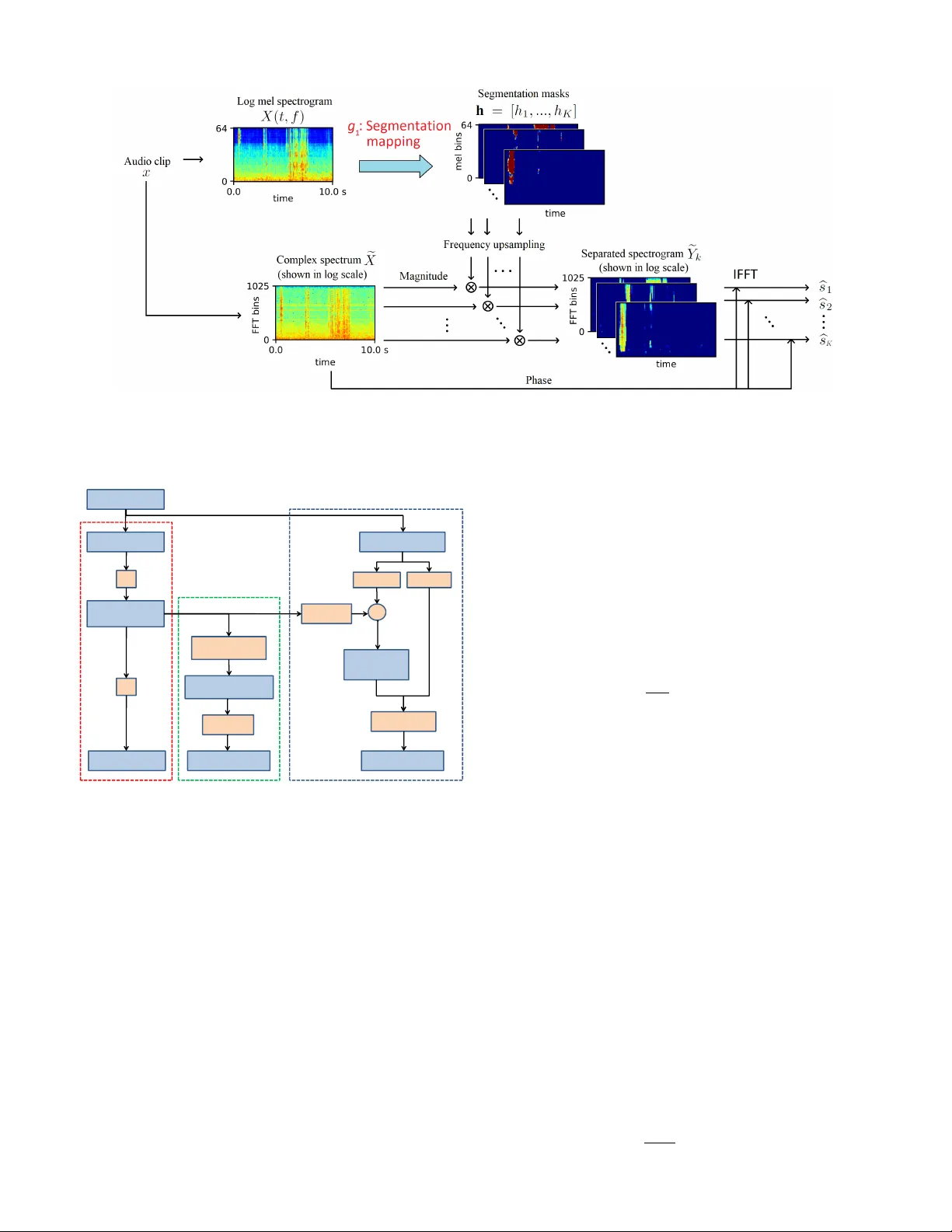
1 Sound Ev ent Detection and T ime-Frequenc y Se gmentation from W eakly Labelled Data Qiuqiang K ong*, Y ong Xu* , Iwona Sobieraj, W enwu W ang, Mark D. Plumbley F ellow , IEEE Abstract —Sound event detection (SED) aims to detect when and recognize what sound e vents happen in an audio clip. Many supervised SED algorithms r ely on strongly labelled data which contains the onset and offset annotations of sound events. Howev er , many audio tagging datasets are weakly labelled, that is, only the presence of the sound e vents is known, without knowing their onset and offset annotations. In this paper , we propose a time-frequency (T -F) segmentation framework trained on weakly labelled data to tackle the sound event detection and separation problem. In training, a segmentation mapping is applied on a T -F repr esentation, such as log mel spectrogram of an audio clip to obtain T -F segmentation masks of sound ev ents. The T -F segmentation masks can be used for separating the sound events from the background scenes in the time-frequency domain. Then a classification mapping is applied on the T -F segmentation masks to estimate the presence pr obabilities of the sound ev ents. W e model the segmentation mapping using a con volutional neural network and the classification mapping using a global weighted rank pooling (GWRP). In SED, predicted onset and offset times can be obtained from the T -F segmentation masks. As a bypr oduct, separated wav eforms of sound events can be obtained fr om the T -F segmentation masks. W e remixed the DCASE 2018 T ask 1 acoustic scene data with the DCASE 2018 T ask 2 sound e vents data. When mixing under 0 dB, the proposed method achiev ed F1 scores of 0.534, 0.398 and 0.167 in audio tagging, frame-wise SED and e vent-wise SED, outperf orming the fully connected deep neural network baseline of 0.331, 0.237 and 0.120, respectiv ely . In T -F segmentation, we achieved an F1 score of 0.218, where previous methods were not able to do T -F segmentation. Index T erms —Sound event detection, time-frequency segmen- tation, weakly labelled data, con volutional neural network. I . I N T RO D U C T I O N Sound event detection (SED) aims to detect what sound ev ents happen in an audio recording and when the y occur . SED has many applications in ev eryday life. For example, SED can be used to monitor “baby cry” sound at home [1], and to detect “typing keyboard”, “door slamming”, “ringing of phones”, “smoke alarms” and “sirens” in the of fice [2, 3]. For public security , SED can be used to detect “gunshot” and “scream” sounds [4]. Not only is SED complementary to video or image based e vent detection [5]–[7] but also has many advantages ov er the two modalities. First, sound does not require illumination, so can be used in dark en vironments. Second, sound can penetrate or mo ve around some obstacles, while objects in video and image are often occluded. Third, some abnormal ev ents such as fire alarms are audio only , so can only be detected by sound. Furthermore, storing and processing sound often consumes less computation resources * The first two authors contributed equally to this work. Fig. 1. From top to bottom: W av eform of an audio clip containing three sound events: “T ambourine”, “scissors” and “computer keyboard”; Log mel spectrogram of the audio clip; Ideal ratio mask (IRM) [9] of sound events. Strongly labelled onset and of fset annotations of sound ev ents; W eak labels. “Silence” is the abbre viated as “sil. ”. The signal-to-noise ratio of this audio clip is 0 dB. than video [8], and as a result, longer sound sequences can be stored in a de vice and faster processing can be obtained using equal computation resources. Many SED algorithms rely on str ongly labelled data [10]–[12] where the onset and offset times of sound ev ents hav e been annotated. The segments between the onset and offset labels are used as target e vents for training, while those outside the onset and offset annotations are used as non-target e vents [11, 12]. Ho we ver , collecting strongly labelled data is time consuming because annotating the onset and of fset times of sound ev ents takes more time than annotating audio clips for classification, so the sizes of strongly labelled datasets are often limited to minutes or a few hours [12, 13]. At the same time there are large amounts of weakly labelled data (WLD) av ailable, where only the presence of the sound ev ents is labelled, without any onset and of fset annotations [14, 15] or the sequence of the sound ev ents. Fig. 1 shows the wa veform of an audio clip containing three non-overlapping sound e vents, the log mel spectrogram of the audio clip, the ideal ratio mask (IRM) [9] of the sound 2 Fig. 2. Audio tagging with con volutional neural network. Input log mel spectrogram is presented to a con volutional neural network including con volutional layers, a global pooling layer and fully connected layers to predict the presence probabilities of audio tags. ev ents, the strongly labelled onset and offset annotations and the weak labels. In this paper we will focus on non-ov erlapping sound ev ents as a starting point. In the real world, sound e vents usually happen in real scenes such as a metro station or an urban park. State-of-the-art SED algorithms only detect the onset and the offset of sound e vents in the time domain but do not separate them from background in the T -F domain. The separation of sound ev ents in the T -F domain can be useful for enhancing and recognizing sound ev ents in audio scenes under low signal-to-noise ratio (SNR). In this paper, we propose a T -F segmentation and sound event detection framework trained using weakly labelled data. This is done by learning T -F segmentation masks implicitly in train- ing with only the clip-lev el audio tags. It means that T -F masks are not known even for the training set: the y are predicted as intermediate results. T -F segmentation masks are equiv alent to the ideal ratio masks (IRM) [9]. An IRM is the ratio of the spectrogram of a sound e vent to the spectrogram of the mixed audio. T -F segmentation masks can be used for SED and sound ev ent separation. In training, a segmentation mapping is applied to the T -F representation such as log mel spectrogram of an audio clip to obtain T -F segmentation masks for sound ev ents. Then a classification mapping is applied to the T -F segmentation masks to output the presence probabilities of sound e vents. In T -F segmentation, with a T -F representation of an audio clip as input, the trained segmentation mapping is used to obtain the T -F segmentation masks. In SED, onset and offset times can be obtained from the T -F segmentation masks. As a byproduct, separated wav eforms of sound ev ents can be obtained from the T -F segmentation masks. This work is an extension of the joint separation-classification model for SED of weakly labelled data [16]. The paper is organized as follo ws. Section II introduces previous work in SED with WLD. Section III describes the proposed T -F segmentation, sound e vent detection and separation framew ork. Section IV describes the implemen- tation details of the proposed framew ork. Section V shows experimental results. Section VI concludes and forecasts future work. I I . W E A K L Y S U P E R V I S E D S O U N D E V E N T D E T E C T I O N Compared to the conv entional SED task, where strongly labelled onset and offset annotations for the training set are giv en, the weakly supervised SED task contains only clip-lev el labels. That is, only the presence of sound ev ents is known in an audio clip, without kno wing the temporal locations of the ev ents. Se veral approaches for weakly supervised SED ha ve recently been proposed, including multiple instance learning and con volutional neural networks. A. Multi-instance learning method One solution to the WLD problem is based on multiple instance learning (MIL) [14, 17]. MIL was first proposed in 1997 for drug activity detection [18]. In MIL for SED, an audio clip is labelled positive for a specified sound ev ent if that sound event occurs at least one time in the audio clip, and labelled negati ve if that sound e vent does not occur in the audio clip. For strongly labelled data, the dataset consists of training pairs { x, y } where x is the feature of a frame in an audio clip and y ∈ { 0 , 1 } K is the strong label of the frame, where K denotes the number of sound classes. For weakly labelled data, features of all frames in an audio clip constitute a bag B = { x t } T t =1 where T is the number of frames in the audio clip. Multiple instance assumption states that the weak labels of a bag are y = max t { y t } T t =1 , where y t is the strong label of the feature x t . The weakly labelled data consists of the training pairs { B , y } . The problem of SED from WLD no w can be cast as learning a classifier to predict the labels of the frames { y t } T t =1 of a bag B = { x t } T t =1 . For the general WLD problem, an MIL framework based on a neural network was proposed in [14, 19]. In [14, 20] a support vector machine (SVM) was used to solve MIL as a maximum margin problem. A negati ve mining method was proposed in [21] that selects negati ve examples according to intra-class v ariance criterion. A concept ranking according to negati ve exemplars (CRANE) algorithm was proposed in [22]. Howe ver , an MIL method tends to underestimate the number of positiv e instances in an audio clip [23]. Furthermore, the MIL method cannot predict the T -F segmentations from the WLD [14]. B. Con volutional neural networks for audio tagging and weakly supervised sound event detection Con volutional neural networks (CNNs) ha ve been success- fully used in many areas including image classification [24], object detection [6], image segmentation [25], speech recog- nition [26, 27] and audio classification [28]. In this section we briefly introduce pre vious work using con v olutional neural network for audio tagging [28] and weakly supervised SED. Audio tagging [12, 28, 29] aims to predict the presence of sound events in an audio clip. In [30], a mel spectrogram of an audio clip is presented to a CNN, where the filters of each con- volutional layer capture local patterns of a spectrogram. After a global pooling layer such as global max pooling [28], global 3 Fig. 3. Training stage using weakly labelled data. A se gmentation mapping g 1 maps from an input T -F representation to the segmentation masks. A classification mapping g 2 maps each segmentation mask to the presence probabilities of the corresponding audio tag. av erage pooling [31], global weighted rank pooling [23], global attention pooling [32, 33] or other poolings [34, 35], fully connected layers are applied to predict the presence probabilities of audio classes. Fig. 2 shows the frame work of audio tagging with con v olutional neural network. Howe ver , this CNN only predicts the presence probabilities of a sound ev ents in an audio clip, but not the onset and offset times of the sound e v ents. In [36, 37], a time-distributed CNN with a global max- pooling strategy was proposed to approximate the MIL method to predict the temporal locations of each event. Howe v er , the global max-pooling will encourage the model to attend to the most dominant T -F unit contributing to the presence of the sound event and ignore all of other T -F units. That is, the hap- pening time of the sound ev ents is underestimated. A method for localizing the sound events in an audio clip by splitting the input into several segments based on the CNNs was presented in [38]. It splits an audio clip into several segments with the assumption that parts of the segments correspond to the clip- lev el labels. This assumption may be unreasonable due to the fact that some sound e vents may only occur at certain frames. Recently , an attention-based global pooling strategy using CNNs was proposed to predict the temporal locations [39] for SED using WLD. Ho wev er , attention-based global pooling can only predict the time domain segmentation, b ut not the T -F se gmentation which will be firstly addressed in this paper . I I I . T I M E - F R E Q U E N C Y S E G M E N TA T I O N , S O U N D E V E N T D E T E C T I O N A N D S E PA R A T I O N F RO M W E A K LY L A B E L L E D DAT A In this section, we present a T -F segmentation, sound ev ent detection and separation framework trained on weakly labelled audio data. Unlike the CNN method for audio tagging, we design a CNN to learn T -F segmentation masks of sound ev ents from the weakly labelled data. A. T raining fr om weakly labelled data W e use only weakly labelled audio data to train the proposed model. The training stage is sho wn in Fig. 3. T o be gin with, the wav eform of an audio clip x is con verted to an input time- frequency (T -F) representation X ( t, f ) , for e xample, spectro- gram or log mel spectrogram. T o simplify the notation, we abbreviate X ( t, f ) as X . The first part of the training stage is a se gmentation mapping g 1 : X 7→ h which maps the input T -F representation to the T -F segmentation masks h = [ h 1 , ..., h K ] , where K is the number of T -F segmentation masks and is equal to the number of sound ev ents. Symbol h k is the abbreviation of h k ( t, f ) which is the T -F segmentation mask of the k -th event. Ideally , each T -F segmentation mask h k is an ideal ratio mask [9] of the k -th sound ev ent. The second part of the training stage is a classification mapping g 2 : h k 7→ p k , k = 1 , ..., K where g 2 maps each T -F se gmentation mask to the presence probability of the k -th ev ent, denoted as p k . Then the binary crossentrop y between the predictions p k , k = 1 , ..., K and the targets y k , k = 1 , ..., K is calculated as the loss function: l ( p k , y k ) = − K X k =1 y k log p k = − K X k =1 y k log g 2 ( g 1 ( X ) k ) , (1) where y k ∈ { 0 , 1 } , k = 1 , ..., K is the binary representation of the weak labels. Both g 1 and g 2 can be modeled by neural networks. The parameters of g 1 and g 2 can be trained end-to- end from the input T -F representation to the weak labels of an audio clip. B. T ime-fr equency segmentation In inference step, the input T -F representation of an audio clip is presented to the segmentation mapping g 1 to obtain the T -F segmentation masks h k , k = 1 , ..., K . The T -F segmenta- tion masks indicate which T -F units in the T -F representation contribute to the presence of the sound ev ents (top right of Fig. 4). The learned T -F segmentation masks are affected by the classification mapping g 2 and will be discussed in Section IV. C. Sound event detection As T -F segmentation masks h k , k = 1 , ..., K contain the information about where sound events happen in the T -F domain, the simplest way to obtain the sound ev ent detection score v k ( t ) in the time domain is to average out the frequency axis of the T -F segmentation masks (bottom right of Fig. 4): v k ( t ) = 1 F F X f =1 h k ( t, f ) , (2) where F is the number of frequency bins of the segmentation mask h k . Then v k ( t ) is the score of the frame-wise prediction 4 Fig. 4. Inference stage. An input T -F representation is presented to the segmentation mapping g 1 to obtain the T -F segmentation masks. By averaging out the frequency axis of the T -F segmentation masks and post processing, ev ent-wise predictions of sound ev ents can be obtained. of the sound events. W e describe ho w to con vert the frame- wise scores to event-wise sound e vents in Section IV -C. D. Sound event separation As a byproduct, the T -F segmentation masks can be used to separate sound ev ents from the mixture in the T -F domain. In addition, by applying an in v erse Fourier transform on the separated T -F representation of each sound e vent, separated wa veforms of the sound ev ents can be obtained. Separating sound e vents from the mixture of sound e v ents and background under a lo w SNR can improve the recognition of sound events in future work. Fig. 5 shows the pipeline of sound e vent separation. An audio clip x is presented to the segmentation mapping g 1 to obtain T -F segmentation masks. Meanwhile, the complex spectrum e X of the audio clip is calculated. W e use the tilde on X to distinguish the complex spectrum e X from the input T -F representation X because X might not be a spectrum, such as log mel spectrogram. W e interpo- late the se gmentation masks of the input T -F representation h k , k = 1 , ..., K to e h k , k = 1 , ..., K representing the T -F segmentation masks of the complex spectrum. The reason for performing this interpolation is that e h k may ha ve a size different from h k , for example, a log mel spectrogram has fewer frequency bins than linear spectrum in the frequency domain. Then we multiply the upsampled T -F segmentation masks e h k with the magnitude of the spectrum to obtain the segmented spectrogram of the k -th ev ent: e Y k = e h k     e X    , k = 1 , ..., K , (3) where  represents the element-wise multiplication and e Y k represents the segmented spectrogram of the k -th ev ent. Fi- nally , an in v erse Fourier transform with overlap add [40] is applied on each segmented spectrogram with the phase from e X to obtain the separated w av eforms b s k , k = 1 , ..., K : b s k = IFFT  e Y k · e j ∠ e X  . (4) W e summarize the training, time-frequency segmentation, sound event detection and separation framew ork in Fig. 6. The training stage, sound event detection stage and sound e vent separation stage are shown in the left, middle and right column of Fig. 6, respectively . I V . P RO P O S E D S E G M E N TA T I O N M A P P I N G A N D C L A S S I FI C A T I O N M A P P I N G In this section, we describe the implementation details of the segmentation mapping g 1 and the classification mapping g 2 proposed in Section III. A. Se gmentation mapping Segmentation mapping g 1 takes a T -F representation of an audio clip as input and outputs segmentation masks of each sound e vent. W e use log mel spectrogram as the input T - F representation, which has been sho wn to perform well in audio classification [28, 39, 41]. Ideally , the outputs of g 1 are ideal ratio masks (IRMs) [42] of sound e vents in the T -F domain. The se gmentation mapping g 1 is modeled by a CNN. Each con v olutional layer consists of a linear con volution, a batch normalization (BN) [43] and a ReLU [44] nonlinearity as in [43]. The BN inserted between the con volution and the nonlinearity can stabilize and speed up the training [43]. W e do not apply do wnsampling layers after con volutional layers because we want to retain the resolution of the input T -F segmentation masks. The T -F segmentation masks are obtained from the activ ations of the last CNN layer using a sigmoid non- linearity to constrain the values of the T -F segmentation masks to be between 0 and 1 to be a valid v alue of an IRM. The configuration details of the CNN will be described in Section V -D. The idea of learning the T -F segmentation masks explicitly is inspired by work on weakly labelled image localization [45] and image segmentation [46, 47]. In weakly labelled image localization, saliency maps are learned indicating the locations of the objects in an image [45]. Similarly , the T -F segmentation masks in our work resemble the saliency maps of an image [45], where T -F se gmentation masks indicate what time and frequency a sound ev ent occurs in a T -F representation. B. Classification mapping As described in Section III, the classification mapping g 1 maps each segmentation mask h k to the presence probability of its corresponding sound e vent. Modeling the classification mapping in different ways will lead to dif ferent representation of the segmentation masks (Fig. 7). W e explored global max pooling [28], global average pooling [31] and global rank pooling [23] for modeling the classification mappings g 2 . 5 Fig. 5. Sound e vent separation stage. An input T -F representation is presented to the segmentation mapping g 1 to obtain the T -F segmentation masks. The upsampled segmentation masks are multiplied with the magnitude spectrum of the input audio to obtain the segmented spectrogram of each sound event. Separated sound events are obtained by applying an in verse Fourier transform to the segmented spectrogram. Wa veform T-F repre sentation T-F Segmentat ion masks g 1 Average along Upsampling Complex spectrogr am × magnitude phase Audio tags g 2 Average along frequency axis Score of s ound events along time axis Separated spectrogram (magnitude) Inverse Fourier transform Separated waveforms Post processing Detected sound events T raining f rom WLD Sound event detection Sound event separation Fig. 6. Framework of T -F se gmentation, sound e vent detection and sound ev ent separation from WLD. From left to right: Training from WLD; Sound ev ent detection; Sound e vent separation. 1) Global max pooling: Global max pooling (GMP) ap- plied on feature maps has been used in audio tagging [28]. GMP on each T -F segmentation mask map h k is depicted as: F ( h k ) = max t,f h k ( t, f ) . (5) GMP is based on the assumption that an audio clip contains a sound ev ent if at least one T -F unit of the T -F input representation contains a sound event. GMP is inv ariant to the location of sound ev ent in the T -F domain because whenev er a sound event occurs, GMP will only select the maximum value of a T -F segmentation mask which is robust to the time or frequency shifts of the sound e vent. Howe ver , in the training stage, back propagation will only pass through the maximum value, so only a small part of data in the T -F domain are used to update the parameters in the neural network. Because of the maximum selection strategy , GMP encourages only one point in a T -F segmentation mask to be positi ve, so GMP will underestimate [23] the sound e vents in the T -F representation. Examples of T -F segmentation masks learned using GMP are shown in Fig. 7(c). 2) Global average pooling: Global av erage pooling (GAP) was first applied in image classification [31]. GAP on each T -F segmentation mask h k is depicted as: F ( h k ) = 1 T F T X t F X f h k ( t, f ) . (6) GAP corresponds to the collectiv e assumption in MIL [48], which states that all T -F units in a T -F se gmentation mask contribute equally to the label of an audio clip. That is, all T - F units in a T -F segmentation mask are assumed to contain the labelled sound ev ents. Howe ver , some sound ev ents only last a short time, so GAP usually overestimates the sound ev ents [31]. Examples of T -F segmentation masks learned using GAP are shown in Fig 7(d). 3) Global weighted rank pooling: T o overcome the lim- itations of GMP and GAP , which underestimate and over - estimate the sound ev ents in the T -F segmentation masks, global weighted rank pooling (GWRP) is proposed in [23]. GWRP can be seen as a generalization of GMP and GAP . The idea of GWRP is to put a descending weight on the values of a T -F se gmentation mask sorted in a descending order . Let an index set I c = { i 1 , ...i M } define the descending order of the v alues within a T -F se gmentation mask h k , i.e. ( h k ) i 1 ≥ ( h k ) i 2 ≥ ... ≥ ( h k ) i n , where M = T × F is the number of T -F units in a T -F segmentation mask. Then the GWRP is defined as: F ( h k ) = 1 Z ( r ) M X j =1 r j − 1 ( h k ) i j , (7) 6 Fig. 7. (a) Spectrogram of an audio clip containing “scissors”, “computer keyboard” and “tambourine” (plotted in log scale); (b) Log mel spectrogram of the audio clip; (c) Upsampled T -F segmentation masks e h k of sound e vents learned using global max pooling (GMP). Only a few T -F units have high value and the other parts of the T -F segmentation masks are dark; (d) Upsampled T -F segmentation masks e h k of sound events learned using global average pooling (GAP); (e) Upsampled T -F segmentation masks e h k of sound ev ents learned using global weighted rank pooling (GWRP); (f) Ideal ratio mask (IRM) of sound ev ents. Only 6 out of 41 T -F segmentation masks are plotted due to the limited space. where 0 ≤ r ≤ 1 is a hyper parameter and Z ( r ) = P M j =1 r j − 1 is a normalization term. When r = 0 GWRP becomes GMP and when r = 1 GWRP becomes GAP . The hyperparameter r can vary depending on the frequency of occurrence of the sound ev ents. GW AP attends more to the T -F units of high values in a T -F segmentation mask and less to those of low values in a T -F segmentation mask. The T -F segmentation masks learned using GWMP is sho wn in Fig. 7(e). The ideal binary masks (IBMs) of the sound events are plotted in Fig. 7(f) for comparison with the GMP , GAP and GWRP . C. P ost-processing for sound event detection In Section III-C we mentioned that the frame-wise scores v k ( t ) can be obtained from the T -F segmentation masks using Equation (2). T o reduce the number of false alarms, for an audio clip, we only apply sound event detection on the sound classes with positive audio tagging predictions. Then we apply thresholds on the frame-wise predictions v k ( t ) to obtain the ev ent-wise predictions. W e apply a high threshold of 0.2 to detect the presence of sound events and then extend the boundary of both onset and of fset sides until the frame-wise scores drop below threshold of 0.1. This two-step threshold method will produce smooth predictions of sound events. As the duration of sound e vents in DCASE 2018 T ask 2 varies from 300 ms to 30 s, we remove the detected sound events that are shorter than 320 ms (10 frames) to reduce false alarms and join the sound e vents whose silence gap is shorter than 320 ms (10 frames). V . E X P E R I M E N T S A. Dataset W e mix the DCASE 2018 T ask 1 acoustic scene dataset [49] with the DCASE 2018 T ask 2 general-purpose Freesound dataset [50] under different signal-to-noise ratios (SNRs) to ev aluate the proposed methods. The reason for this choice is that DCASE 2018 T ask 1 provides background sounds recorded from a variety of real world scenes whereas the DCASE 2018 T ask 2 provides a variety of foreground sound ev ents. The DCASE 2018 T ask 1 contains 8640 10-second audio clips in the de velopment set of subtask A. The audio clips are recorded from 10 different scenes such as “airport”, “metro station” and “urban park”. The DCASE 2018 T ask 2 contains 3710 manually v erified sound events ranging in length from 300 ms to 30 s depending on the audio classes. There are 41 classes of sound e vents such as “flute”, “applause” and “cough”. W e only use these manually verified audio clips from the DCASE 2018 T ask 2 as sound e vents because the remaining audio clips are un verified and may contain noisy labels. W e truncated the sound events to up to 2 seconds and mix them with the 10-second audio clips from the DCASE 2018 T ask 1 acoustic scene dataset. The mixed audio clips are single channel with a sampling rate of 32 kHz. Each mixed audio clip contains three non-o verlapped sound events. W e mixed the sound events with the acoustic scenes for SNRs at 20dB, 10dB and 0dB. F or each SNR, the 8000 mixed audio clips are divided into 4 cross-validation folds. Fig. 7(b) sho ws the log mel spectrogram of a mix ed 10-second audio clip. The source code of our w ork is released 1 . B. Evaluation metrics W e use F-score [51], area under the curve (A UC) [52] and mean av erage precision (mAP) [6] in the e v aluation of the audio tagging, the frame-wise SED and the T -F segmentation. W e also use error rate (ER) for ev aluating the event-wise SED. 1) Basic statistics: T rue positiv e (TP): Both the reference and the system prediction indicate an ev ent to be active. False negati ve (FN): The reference indicates an e vent to be active but the system prediction indicates an ev ent to be inactive. False positiv e (FP): The system prediction indicates an ev ent to be acti v e but the reference indicates it is not [51]. 1 https://github .com/qiuqiangkong/sed_time_freq_segmentation 7 2) Pr ecision, r ecall and F-score: Precision ( P ) and recall ( R ) are defined as [51]: P = T P T P + F P , R = T P T P + F N . (8) Bigger P and R indicates better performance. F-score is calculated based on P and R [51]: F = 2 P · R P + R = T P T P + ( F N + F P ) / 2 . (9) Bigger F-score indicates better performance. 3) Ar ea under the curve (A UC): A receiver operating characteristic (R OC) curve [52] plots true positiv e rate (TPR) versus false positiv e rate (FPR). Area under the curv e (A UC) score is the area under this R OC curve which summarizes the R OC curve to a single number . Using the A UC does not require manual selection of a threshold. Bigger A UC indicates better performance. A random guess has an A UC of 0.5. 4) A verag e pr ecision: A verage precision (AP) is the av er- age of the precision at different recall values. Similar to A UC, AP does not rely on the threshold. Dif ferent to A UC, AP does not count the true neg ativ es and is widely used as a criterion in imbalanced dataset such as object detection [6]. 5) Err or rate: Error rate (ER) is an e vent-wise ev aluation metric. ER measures the amount of errors in terms of inser- tions (I), deletions (D) and substitutions (S) [51]. For an audio clip, the insertions, deletions and substitutions are defined as: S = min ( F N , F P ) , D = max (0 , F N − F P ) , I = max (0 , F P − F N ) , (10) where FN, FP , FN are e vent-wise statistics in an audio clip. Lower ER , S , D and I indicate the better performance. When ev aluating the ev ent based criterion, we allow some degree of misalignment between a reference and a system output for counting a true positi ve [12, 51, 53]. Follo wing the default configuration of [51], we adopt an onset collar of 200 ms and an offset collar of 200 ms / 50% to count the true positiv e of a detection. W e used the toolbox [51] for e valuating the performance of the event-based SED. C. F eatur e extr action W e apply a fast Fourier transform (FFT) with a windo w size of 2048 and an overlap of 1024 between neighbouring windows to extract the spectrogram of audio clips. This configuration that follows [54] offers a good resolution in both time and frequenc y domain. Then mel filter banks with 64 bands are applied on the spectrogram follo wed by logarithm operation to obtain log mel spectrogram as the input T -F representation feature. Log mel spectrogram has been widely used in audio classification [28, 54]. D. Model In this subsection we gi ve a detailed description of the configuration of the segmentation mapping in Section IV -A and the classification mapping in Section IV -B. W e apply a T ABLE I C O NFI G U R A TI O N O F C N N . Layers Output size (feature maps × time steps × mel bins) Input log mel spectrogram 1 × 311 × 64 { 3 × 3 , 32 , BN , ReLU } × 2 32 × 311 × 64 { 3 × 3 , 64 , BN , ReLU } × 2 64 × 311 × 64 { 3 × 3 , 128 , BN , ReLU } × 2 128 × 311 × 64 { 3 × 3 , 128 , BN , ReLU } × 2 128 × 311 × 64 1 × 1 , 41 , sigmoid 41 × 311 × 64 Global pooling (GP) 41 T ABLE II F 1 - S C O R E , AUC A ND M AP OF AU DI O T AG G I NG A T D I FF ER E N T S N R S . 20 dB 10 dB 0 dB Algorithms F1 A UC mAP F1 A UC mAP F1 A UC mAP DNN [55] 0.439 0.885 0.468 0.396 0.861 0.402 0.331 0.810 0.314 WLD CNN [37] 0.498 0.777 0.498 0.524 0.794 0.526 0.528 0.815 0.535 FrameCNN [34] 0.581 0.899 0.587 0.543 0.883 0.526 0.484 0.850 0.439 Attention [39] 0.714 0.922 0.755 0.690 0.907 0.729 0.612 0.875 0.643 GMP 0.435 0.818 0.475 0.406 0.801 0.440 0.373 0.773 0.389 GAP 0.529 0.934 0.623 0.467 0.914 0.555 0.385 0.877 0.442 GWRP 0.635 0.955 0.753 0.604 0.942 0.696 0.534 0.915 0.596 “VGG-like” conv olutional neural netw ork [56] with 8 conv o- lutional blocks on the input log mel spectrogram [54]. Each con volutional layer consists of a linear con volution with a filter size of 3 × 3 followed by a batch normalization layer [43] and a ReLU activ ation function [44]. W e use 4 conv olution blocks following the baseline system of DCASE 2018 [54]. The number of feature maps of the con volutional layers are 32, 64, 128 and 128, respecti v ely . This configuration is to fit the model to a single GPU card with 12 GB RAM sufficiently . Then a 1 × 1 con v olutional layer with sigmoid non-linearity is applied to conv ert the feature maps to the T -F segmentation masks of sound e vents. Then a global pooling is used to summarize each T -F segmentation mask to a scalar representing the presence probability of the sound e vents in an audio clip. W e summarize the configuration of the neural network in T able I. In training we use a mini-batch size of 24 to fully utilize the single card GPU with 12 GB RAM. The Adam optimizer [57] with a learning rate 0.001 is used for its fast con ver gence. E. A udio tagging W e compare our method with fully connected neural network [55], CNN trained on weakly labelled data [37], FrameCNN [34] and the attention model [39]. W e apply GMP , GAP and GWRP as global pooling in our model. T able II shows that for SNR at 20 dB, the attention model [39] achie ves the best F1-score of 0.714 and mAP of 0.755 follo wed by the GWRP of 0.635 and 0.753, respecti vely . On the other hand, GWRP achiev es the best A UC of 0.955. Comparing the performance under different SNRs, the F1-score and mAP drop approximately 0.1 in absolute value for SNR changed from 20 dB to 0 dB. A UC drop approximately 0.04 in absolute 8 T ABLE III F 1 - S C O R E O F AU D IO T AG G I N G A T 0 D B S NR . Acous. guitar Appla- use Bark Bass drum Burp- ing Bus Cello Chime Clari- net Keybo- ard Cough Cow- bell Double bass Drawer Elec. piano Fart Finger snap Fire- works Flute Glock- enspiel Gong DNN [55] 0.286 0.873 0.332 0.041 0.344 0.367 0.489 0.546 0.423 0.283 0.075 0.133 0.197 0.083 0.304 0.267 0.389 0.285 0.350 0.464 0.310 WLD CNN [37] 0.633 0.896 0.719 0.547 0.794 0.248 0.610 0.589 0.504 0.390 0.513 0.889 0.436 0.136 0.435 0.384 0.672 0.375 0.270 0.692 0.513 FrameCNN [34] 0.416 0.878 0.719 0.166 0.557 0.385 0.529 0.562 0.448 0.507 0.484 0.668 0.314 0.181 0.392 0.304 0.556 0.474 0.385 0.488 0.465 Attention [39] 0.548 0.893 0.761 0.632 0.866 0.335 0.616 0.607 0.568 0.497 0.565 0.924 0.477 0.160 0.546 0.598 0.823 0.463 0.565 0.901 0.617 GMP 0.458 0.522 0.335 0.183 0.400 0.087 0.299 0.468 0.424 0.422 0.151 0.774 0.281 0.076 0.279 0.284 0.176 0.271 0.315 0.844 0.434 GAP 0.547 0.817 0.409 0.070 0.484 0.205 0.435 0.501 0.354 0.504 0.347 0.314 0.181 0.164 0.218 0.407 0.399 0.346 0.343 0.496 0.305 GWRP 0.552 0.825 0.654 0.204 0.578 0.342 0.416 0.628 0.424 0.573 0.543 0.579 0.333 0.320 0.421 0.618 0.473 0.558 0.427 0.726 0.550 Gunshot Harmo- nica Hi- hat Keys Knock Laugh- ter Meow Micro- wav e Oboe Saxo- phone Sciss- ors Shatter Snare drum Squeak T ambo- urine T ear- ing T ele- phone Trumpet Violin Writ- ing A vg. DNN [55] 0.297 0.672 0.547 0.418 0.276 0.192 0.075 0.121 0.408 0.500 0.411 0.336 0.368 0.097 0.299 0.254 0.270 0.528 0.379 0.293 0.331 WLD CNN [37] 0.538 0.742 0.910 0.643 0.649 0.361 0.359 0.263 0.589 0.636 0.558 0.410 0.599 0.052 0.593 0.436 0.324 0.642 0.755 0.349 0.528 FrameCNN [34] 0.424 0.723 0.688 0.660 0.553 0.390 0.355 0.400 0.490 0.528 0.497 0.481 0.624 0.193 0.733 0.449 0.346 0.526 0.475 0.431 0.484 Attention [39] 0.607 0.759 0.938 0.744 0.738 0.444 0.499 0.441 0.560 0.678 0.660 0.693 0.709 0.113 0.957 0.593 0.434 0.368 0.784 0.400 0.612 GMP 0.398 0.322 0.796 0.141 0.483 0.311 0.275 0.207 0.442 0.474 0.173 0.251 0.465 0.031 0.891 0.504 0.329 0.585 0.567 0.175 0.373 GAP 0.438 0.681 0.641 0.392 0.402 0.480 0.203 0.172 0.372 0.408 0.404 0.392 0.335 0.161 0.412 0.348 0.341 0.579 0.349 0.408 0.385 GWRP 0.523 0.714 0.798 0.606 0.524 0.563 0.547 0.353 0.487 0.534 0.452 0.653 0.585 0.260 0.857 0.583 0.508 0.639 0.516 0.452 0.534 T ABLE IV F 1 - S C O R E O F F R AM E - W IS E S E D AT 0 D B S N R . Acous. guitar Appla- use Bark Bass drum Burp- ing Bus Cello Chime Clari- net Keybo- ard Cough Cow- bell Double bass Drawer Elec. piano Fart Finger snap Fire- works Flute Glock- enspiel Gong DNN [55] 0.191 0.746 0.239 0.009 0.317 0.306 0.373 0.495 0.295 0.202 0.036 0.050 0.123 0.038 0.233 0.207 0.156 0.195 0.214 0.291 0.212 WLD CNN [37] 0.113 0.466 0.159 0.052 0.292 0.044 0.318 0.298 0.223 0.100 0.142 0.111 0.097 0.020 0.078 0.078 0.085 0.085 0.042 0.095 0.037 FrameCNN [34] 0.294 0.741 0.585 0.07 0.411 0.299 0.441 0.480 0.342 0.421 0.370 0.283 0.178 0.102 0.310 0.239 0.236 0.325 0.246 0.315 0.308 Attention [39] 0.062 0.422 0.069 0.020 0.189 0.024 0.242 0.263 0.210 0.019 0.059 0.051 0.045 0.003 0.068 0.050 0.076 0.031 0.159 0.026 0.088 GMP 0.000 0.000 0.000 0.000 0.000 0.000 0.000 0.000 0.000 0.000 0.000 0.000 0.000 0.000 0.000 0.000 0.000 0.000 0.000 0.000 0.000 GAP 0.410 0.661 0.338 0.033 0.341 0.139 0.240 0.429 0.195 0.426 0.269 0.121 0.088 0.108 0.170 0.297 0.102 0.229 0.173 0.214 0.200 GWRP 0.453 0.704 0.507 0.072 0.456 0.188 0.326 0.575 0.341 0.457 0.402 0.222 0.193 0.172 0.351 0.498 0.247 0.355 0.316 0.596 0.418 Gunshot Harmo- nica Hi- hat Keys Knock Laugh- ter Meow Micro- wav e Oboe Saxo- phone Sciss- ors Shatter Snare drum Squeak T ambo- urine T ear- ing T ele- phone Trumpet Violin Writ- ing A vg. DNN [55] 0.155 0.594 0.510 0.367 0.16 0.111 0.022 0.095 0.314 0.317 0.277 0.254 0.290 0.045 0.166 0.144 0.190 0.411 0.166 0.212 0.237 WLD CNN [37] 0.093 0.333 0.135 0.160 0.149 0.086 0.056 0.058 0.132 0.234 0.150 0.075 0.141 0.003 0.195 0.055 0.123 0.287 0.258 0.067 0.140 FrameCNN [34] 0.259 0.595 0.639 0.495 0.354 0.271 0.228 0.284 0.399 0.329 0.379 0.364 0.453 0.111 0.443 0.277 0.237 0.407 0.228 0.299 0.343 Attention [39] 0.029 0.143 0.107 0.096 0.101 0.051 0.034 0.018 0.137 0.353 0.078 0.038 0.054 0.005 0.188 0.046 0.148 0.08 0.156 0.056 0.100 GMP 0.000 0.000 0.000 0.000 0.000 0.000 0.000 0.000 0.000 0.000 0.000 0.000 0.000 0.000 0.000 0.000 0.000 0.000 0.000 0.000 0.000 GAP 0.231 0.528 0.553 0.332 0.233 0.294 0.133 0.121 0.237 0.167 0.146 0.319 0.265 0.114 0.191 0.274 0.172 0.437 0.105 0.313 0.252 GWRP 0.362 0.649 0.696 0.539 0.354 0.429 0.400 0.182 0.404 0.440 0.384 0.471 0.373 0.173 0.591 0.378 0.420 0.528 0.331 0.360 0.398 T ABLE V F 1 - S C O R E , AUC A ND M AP OF F RA M E - WI S E S E D AT D IFF E R E NT S NR S . 20 dB 10 dB 0 dB Algorithms F1 A UC mAP F1 A UC mAP F1 A UC mAP DNN [55] 0.360 0.722 0.269 0.306 0.702 0.224 0.237 0.666 0.169 WLD CNN [37] 0.168 0.669 0.179 0.182 0.688 0.201 0.140 0.701 0.166 FrameCNN [34] 0.440 0.808 0.369 0.399 0.787 0.329 0.343 0.756 0.275 Attention [39] 0.163 0.827 0.317 0.137 0.807 0.278 0.100 0.773 0.221 GMP 0.000 0.676 0.090 0.000 0.658 0.076 0.000 0.649 0.072 GAP 0.398 0.790 0.400 0.334 0.753 0.328 0.252 0.712 0.245 GWRP 0.511 0.886 0.508 0.472 0.871 0.453 0.398 0.829 0.360 T ABLE VI F 1 - S C O R E , AUC A ND M AP OF E VE N T - W I SE S ED A T D I FFE R E N T S NR S . 20 dB 10 dB 0 dB Algorithms F1 ER D I F1 ER D I F1 ER D I DNN [55] 0.226 1.91 0.75 1.16 0.178 2.29 0.79 1.50 0.120 2.80 0.84 1.96 WLD CNN [37] 0.010 1.16 0.99 0.17 0.011 1.15 0.99 0.17 0.018 1.12 0.99 0.13 FrameCNN [34] 0.166 2.38 0.79 1.58 0.151 2.49 0.81 1.68 0.141 2.70 0.81 1.88 Attention [39] 0.028 1.10 0.96 0.14 0.021 1.10 0.97 0.13 0.011 1.09 0.98 0.10 GMP 0.000 1.00 1.00 0.00 0.000 1.00 1.00 0.00 0.000 1.00 1.00 0.00 GAP 0.173 2.71 0.78 1.93 0.139 2.95 0.82 2.13 0.098 3.52 0.86 2.66 GWRP 0.254 2.12 0.66 1.45 0.227 2.30 0.69 1.61 0.167 2.55 0.76 1.78 value for SNR changed from 20 dB to 0 dB. This result shows that there is a large variance in audio tagging under low SNR. T able III sho ws the audio tagging results of all sound e vents under 0 dB SNR. Some sound e vents such as “hi-hat” and “tambourine” ha ve higher classification accuracy while some sound e v ents such as “micro wa ve” and “squeak” are dif ficult to recognize. On average, the attention model [39] achie ves the best F1-score of 0.612 followed by GWRP of 0.534. F . F rame-wise sound e vent detection T able IV shows the F1-score of the frame-wise SED for all sound classes under SNR of 0 dB. GWRP achieves the best av eraged F1-score of 0.398, followed by the FrameCNN model [34] of 0.343. Some classes such as “applause” and “hi-hat” ha ve higher F1-score by the frame-wise SED, while some classes such as “drawer” and squeak” have lo wer F1- score by the frame-wise SED. T able V shows the frame-wise SED results under dif ferent SNRs. GWRP achiev es the best F1-score, A UC and mAP of 0.511, 0.886 and 0.508 under 20 dB SNR. The FrameCNN model [34] achie ves a second place with an F1-score of 0.440. GAP overestimates the sound ev ents which is shown in the visualization of the upsampled T - F segmentation masks (Fig. 7). GAP does not perform better than GWRP . GMP underestimates the sound ev ents (Fig. 7) and performs worst in frame-wise SED. In GWRP , the F1- score drops from 0.511 to 0.472 to 0.398 under SNRs of 20 dB, 10 dB and 0 dB. Fig. 8 shows the frame-wise scores of sound e vents obtained from equation (2) under SNR of 0 dB. Frame-wise scores obtained by using GWRP looks 9 T ABLE VII F 1 - S C O R E O F E V EN T - W I S E S E D AT 0 D B SN R . Acous. guitar Appla- use Bark Bass drum Burp- ing Bus Cello Chime Clari- net Keybo- ard Cough Cow- bell Double bass Drawer Elec. piano Fart Finger snap Fire- works Flute Glock- enspiel Gong DNN [55] 0.132 0.287 0.083 0.002 0.176 0.233 0.125 0.389 0.041 0.141 0.033 0.007 0.068 0.036 0.141 0.113 0.035 0.113 0.036 0.079 0.159 WLD CNN [37] 0.020 0.013 0.001 0.001 0.110 0.001 0.036 0.067 0.025 0.005 0.001 0.001 0.003 0.001 0.001 0.001 0.001 0.001 0.001 0.001 0.001 FrameCNN [34] 0.098 0.510 0.187 0.012 0.090 0.180 0.287 0.186 0.157 0.194 0.144 0.005 0.04 0.091 0.168 0.163 0.042 0.133 0.081 0.265 0.098 Attention [39] 0.000 0.051 0.000 0.000 0.052 0.000 0.020 0.018 0.000 0.000 0.000 0.000 0.009 0.000 0.000 0.000 0.000 0.000 0.019 0.000 0.000 GMP 0.000 0.000 0.000 0.000 0.000 0.000 0.000 0.000 0.000 0.000 0.000 0.000 0.000 0.000 0.000 0.000 0.000 0.000 0.000 0.000 0.000 GAP 0.060 0.416 0.141 0.000 0.150 0.035 0.123 0.178 0.085 0.296 0.107 0.016 0.033 0.070 0.025 0.197 0.003 0.078 0.054 0.000 0.032 GWRP 0.131 0.225 0.315 0.002 0.352 0.030 0.086 0.363 0.086 0.211 0.228 0.010 0.089 0.111 0.153 0.312 0.068 0.144 0.060 0.004 0.281 Gunshot Harmo- nica Hi- hat Keys Knock Laugh- ter Meow Micro- wav e Oboe Saxo- phone Sciss- ors Shatter Snare drum Squeak T ambo- urine T ear- ing T ele- phone Trumpet Violin Writ- ing A vg. DNN [55] 0.073 0.455 0.205 0.262 0.095 0.054 0.024 0.047 0.135 0.107 0.128 0.174 0.106 0.020 0.057 0.088 0.100 0.140 0.031 0.173 0.120 WLD CNN [37] 0.001 0.153 0.001 0.003 0.008 0.003 0.001 0.001 0.007 0.043 0.005 0.001 0.011 0.001 0.001 0.001 0.073 0.077 0.063 0.001 0.018 FrameCNN [34] 0.044 0.226 0.409 0.142 0.071 0.113 0.140 0.120 0.223 0.077 0.140 0.134 0.132 0.042 0.031 0.104 0.071 0.241 0.052 0.124 0.141 Attention [39] 0.000 0.000 0.000 0.000 0.106 0.000 0.000 0.000 0.000 0.188 0.000 0.000 0.000 0.000 0.000 0.000 0.000 0.000 0.000 0.000 0.011 GMP 0.000 0.000 0.000 0.000 0.000 0.000 0.000 0.000 0.000 0.000 0.000 0.000 0.000 0.000 0.000 0.000 0.000 0.000 0.000 0.000 0.000 GAP 0.035 0.440 0.002 0.103 0.095 0.152 0.062 0.064 0.153 0.024 0.041 0.024 0.075 0.078 0.003 0.078 0.038 0.257 0.013 0.184 0.098 GWRP 0.078 0.519 0.031 0.356 0.206 0.205 0.269 0.118 0.252 0.165 0.167 0.130 0.065 0.067 0.065 0.146 0.238 0.175 0.105 0.243 0.167 T ABLE VIII F 1 - S C O R E O F T I ME - F RE Q U E NC Y S E G M EN TA T IO N A T 0 D B S N R . Acous. guitar Appla- use Bark Bass drum Burp- ing Bus Cello Chime Clari- net Ke ybo- ard Cough Cow- bell Double bass Drawer Elec. piano Fart Finger snap Fire- works Flute Glock- enspiel Gong GMP 0.000 0.001 0.001 0.000 0.002 0.000 0.003 0.002 0.002 0.002 0.000 0.005 0.001 0.000 0.001 0.000 0.000 0.001 0.001 0.002 0.002 GAP 0.128 0.391 0.106 0.009 0.155 0.073 0.124 0.187 0.057 0.201 0.143 0.038 0.044 0.068 0.067 0.126 0.029 0.119 0.052 0.081 0.116 GWRP 0.222 0.519 0.226 0.030 0.291 0.095 0.213 0.313 0.114 0.303 0.241 0.125 0.086 0.100 0.127 0.256 0.092 0.204 0.104 0.212 0.237 Gunshot Harmo- nica Hi- hat Ke ys Knock Laugh- ter Meow Micro- wav e Oboe Saxo- phone Sciss- ors Shatter Snare drum Squeak T ambo- urine T ear- ing T ele- phone Trumpet V iolin Writ- ing A vg. GMP 0.001 0.002 0.001 0.002 0.001 0.001 0.000 0.000 0.001 0.001 0.000 0.000 0.002 0.000 0.001 0.001 0.001 0.002 0.003 0.001 0.001 GAP 0.139 0.264 0.212 0.139 0.074 0.135 0.085 0.055 0.077 0.120 0.085 0.144 0.108 0.082 0.057 0.140 0.059 0.166 0.074 0.130 0.114 GWRP 0.283 0.379 0.497 0.311 0.190 0.249 0.185 0.085 0.140 0.257 0.213 0.272 0.196 0.108 0.327 0.237 0.138 0.313 0.222 0.215 0.218 T ABLE IX F 1 - S C O R E , AUC A ND M AP OF T IM E - F RE Q U EN C Y S E G ME N TA T IO N AT D I FFE R E N T S N R S . 20 dB 10 dB 0 dB Algorithms F1 A UC mAP F1 A UC mAP F1 A UC mAP GMP 0.001 0.347 0.008 0.001 0.345 0.007 0.001 0.362 0.005 GAP 0.215 0.889 0.230 0.168 0.880 0.187 0.114 0.861 0.143 GWRP 0.324 0.849 0.268 0.280 0.845 0.227 0.218 0.836 0.175 closer to the ground truth than obtained using GMP and GAP . Compared with ev ent-wise SED, frame-wise SED does not depend on post-processing. G. Event-wise sound e vent detection Although frame-wise SED does not depend on post- processing so is a more objectiv e criterion, it mak es more sense to hav e ev ent-wise predictions. The event-wise pre- dictions are obtained from frame-wise predictions following Section IV -C. T able VI shows that the GWRP achie ves the best F1-score of 0.254 in e vent-wise SED. Although GMP seems to achie ve the lo west ER of 1.00, GMP deletes all the ev ents and has a deletion error of 1.00 and an insertion of 0. On the other hand, GWRP has the lowest deletion error of 0.66 and has an insertion error of 1.45. The F1-scores drop from 0.254 to 0.227 to 0.167 under SNRs of 20 dB, 10 dB and 0 dB. T able VII sho ws the the F1-score of e vent-wise SED of all sound classes. Some sound classes such as “barks”, “harmonica” have higher detection F1-score. GWRP achie ves the best a veraged F1-score of 0.167. Fig. 8. Frame-wise predictions using GMP , GAP , GWRP with SNR at 0 dB. The ground truth annotation is shown in the bottom right. H. T ime-fr equency segmentation T able VIII shows the T -F segmentation results of all sound classes under 0 dB. As the T -F segmentation can not be obtained by pre vious works including the fully connected neural network [55], the CNN trained on weakly labelled data 10 [37], the FrameCNN [34] and the attention model [39], we only report the T -F segmentation results with our proposed methods. GWRP achiev es the best F1-score of 0.218 on av erage. T able IX shows the T -F segmentation results under different SNRs. T able IX sho ws that GWRP achieves the best F1-score, A UC and mAP of 0.324, 0.849 and 0.268 under 20 dB SNR, respectively . GMP underestimates the T -F segmenta- tion masks and performs the worst in T -F segmentation. GAP ov erestimates the T -F segmentation masks and performs worse than GWRP in F1-score. The T -F segmentation masks learned by GWRP (Fig. 7(e)) looks closer to the IRM than the T -F segmentation masks learned by using GMP and GAP . V I . C O N C L U S I O N This paper proposes a time-frequency (T -F) segmentation, sound ev ent detection and separation framework trained on weakly labelled data. In training, a segmentation mapping and a classification mapping are trained jointly using the weakly labelled data. In T -F segmentation, we use the trained seg- mentation mapping to calculate the T -F segmentation masks. Detected sound e vents can then be obtained from the T -F segmentation masks. As a byproduct, separated wav eforms of sound e vents can be obtained from the T -F segmentation masks. Experiments show that the global weighted rank pool- ing (GWRP) outperforms the global max pooling, the global av erage pooling and previously proposed systems in both of T -F segmentation and sound event detection. The limitation of this approach is that the T -F se gmentation masks are not perfectly matching the ideal ratio mask (IRM) of the sound ev ents. In future, we will impro ve the T -F segmentation masks to match the IRM for event separation. A C K N O W L E D G M E N T This research was supported by EPSRC grant EP/N014111/1 “Making Sense of Sounds” and a Research Scholarship from the China Scholarship Council (CSC) No. 201406150082. Iwona Sobieraj is sponsored by the European Union’ s H2020 Framework Programme (H2020-MSCA-ITN- 2014) under grant agreement No. 642685 MacSeNet. The authors thank Dominic W ard for helping to improve the paper in the early stage. The authors thank all anonymous revie wers for their ef fort and suggestions to improve this paper . R E F E R E N C E S [1] J. Saraswathy , M. Hariharan, S. Y aacob, and W . Khairunizam. Automatic classification of infant cry: A review . In Pr oceedings of the International Confer ence on Biomedical Engineering (ICoBE) , pages 543–548, 2012. [2] A. Harma, M. F . McKinney , and J. Skowronek. Automatic surveillance of the acoustic activity in our living en vironment. In Pr oceedins of the IEEE International Confer ence on Multimedia and Expo (ICME) , pages 634–637, 2005. [3] D. P . W . Ellis. Detecting alarm sounds. In Pr oceedings of the Consistent & Reliable Acoustic Cues for Sound Analysis W orkshop (CRAC ’01) , pages 59–62, 2001. [4] G. V alenzise, L. Gerosa, M. T agliasacchi, F . Antonacci, and A. Sarti. Scream and gunshot detection and localization for audio-surv eillance systems. In Pr oceedings of the IEEE Confer ence on Advanced V ideo and Signal Based Surveillance (A VSS) , pages 21–26, 2007. [5] Z. Xu, Y . Y ang, and A. G. Hauptmann. A discriminative CNN video representation for event detection. In Pr oceedings of the IEEE Confer ence on Computer V ision and P attern Recognition (CVPR) , pages 1798–1807, 2015. [6] R. Girshick, J. Donahue, T . Darrell, and J. Malik. Rich feature hierarchies for accurate object detection and semantic segmentation. In Pr oceedings of the IEEE Conference on Computer V ision and P attern Recognition (CVPR) , pages 580–587, 2014. [7] A. Borji, M. Cheng, H. Jiang, and J. Li. Salient object detection: A benchmark. IEEE T ransactions on Image Processing , 24(12):5706– 5722, 2015. [8] Sami Abu-El-Haija, Nisarg Kothari, Joonseok Lee, Paul Natsev , George T oderici, Balakrishnan V aradarajan, and Sudheendra V ijayanarasimhan. Y ouT ube-8M: A large-scale video classification benchmark. arXiv pr eprint arXiv:1609.08675 , 2016. [9] A. Narayanan and D. W ang. Ideal ratio mask estimation using deep neural networks for rob ust speech recognition. In Pr oceedings of the IEEE International Conference on Acoustics, Speec h and Signal Pr ocessing (ICASSP) , pages 7092–7096, 2013. [10] D. Stowell, D. Giannoulis, E. Benetos, M. Lagrange, and M. D. Plumbley . Detection and classification of acoustic scenes and events. IEEE T ransactions on Multimedia , 17(10):1733–1746, 2015. [11] G. P arascandolo, H. Huttunen, and T . V irtanen. Recurrent neural networks for polyphonic sound event detection in real life recordings. In Pr oceedings of the IEEE International Conference on Acoustics, Speech and Signal Processing (ICASSP) , pages 6440–6444, 2016. [12] A. Mesaros, T . Heittola, and T . V irtanen. TUT database for acoustic scene classification and sound event detection. In Proceedings of the 24th European Signal Pr ocessing Conference (EUSIPCO) , pages 1128– 1132, 2016. [13] D. Giannoulis, E. Benetos, D. Sto well, M. Rossignol, M. Lagrange, and M. D. Plumbley . Detection and classification of acoustic scenes and ev ents: an IEEE AASP challenge. In Pr oceedings of the IEEE W orkshop on Applications of Signal Pr ocessing to Audio and Acoustics (W ASP AA) , 2013. [14] A. K umar and B. Raj. Audio event detection using weakly labeled data. In Pr oceedings of the 2016 ACM on Multimedia Conference , pages 1038–1047, 2016. [15] S. Adav anne and T . V irtanen. Sound ev ent detection using weakly labeled dataset with stacked con volutional and recurrent neural netw ork. T echnical report, DCASE2017 Challenge, September 2017. [16] Qiuqiang Kong, Y ong Xu, W enwu W ang, and Mark D Plumble y . A joint separation-classification model for sound event detection of weakly labelled data. In Proceedings of the IEEE International Conference on Acoustics, Speech and Signal Processing (ICASSP) , pages 321–325, 2017. [17] O. Maron and T . Lozano-Pérez. A framework for multiple-instance learning. In Pr oceedings of the Advances in Neural Information Pr ocessing Systems (NIPS) , volume 10, pages 570–576, 1998. [18] Thomas G Dietterich, Richard H Lathrop, and T omás Lozano-Pérez. Solving the multiple instance problem with axis-parallel rectangles. Artificial intelligence , 89(1-2):31–71, 1997. [19] Z. Zhou and M. Zhang. Neural networks for multi-instance learning. In Pr oceedings of the International Confer ence on Intelligent Information T echnology (ICIIT) , pages 455–459, 2002. [20] S. Andrews, I. Tsochantaridis, and T . Hofmann. Support vector machines for multiple-instance learning. In Proceedings of the Advances in Neural Information Processing Systems (NIPS) , volume 15, pages 577–584, 2003. [21] P . Si va, C. Russell, and T . Xiang. In defence of neg ative mining for annotating weakly labelled data. In Proceedings of the Eur opean Confer ence on Computer V ision (ECCV) , pages 594–608, 2012. [22] K. T ang, R. Sukthankar, J. Y agnik, and L. Fei-Fei. Discriminative segment annotation in weakly labeled video. In Proceedings of the IEEE Conference on Computer V ision and P attern Recognition (CVPR) , pages 2483–2490, 2013. [23] A. Kolesnik ov and C. H. Lampert. Seed, expand and constrain: Three principles for weakly-supervised image segmentation. In Proceedings of the Eur opean Conference on Computer V ision (ECCV) , pages 695–711, 2016. [24] A. Krizhe vsky , I. Sutskev er , and G. E. Hinton. ImageNet classification with deep conv olutional neural networks. In Pr oceedings of the Ad- vances in Neural Information Pr ocessing Systems (NIPS) , volume 25, pages 1097–1105, 2012. [25] J. Long, E. Shelhamer , and T . Darrell. Fully con volutional networks for semantic segmentation. In Proceedings of the IEEE Conference on Computer V ision and P attern Recognition (CVPR) , pages 3431–3440, 2015. [26] G. E. Dahl, D. Y u, L. Deng, and A. Acero. Context-dependent pre-trained deep neural networks for large-vocab ulary speech recogni- 11 tion. IEEE Tr ansactions on Audio, Speech, and Language Processing , 20(1):30–42, 2012. [27] O. Abdel-Hamid, A. Mohamed, H. Jiang, L. Deng, G. Penn, and D Y u. Con volutional neural networks for speech recognition. IEEE/ACM T ransactions on A udio, Speech, and Language Pr ocessing , 22(10):1533– 1545, 2014. [28] K. Choi, G. Fazekas, and M. Sandler . Automatic tagging using deep con volutional neural netw orks. In Pr oceedings of the 17th International Confer ence on Music Information Retrie val (ISMIR) , pages 805–811, 2016. [29] P . F oster , S. Sigtia, S. Krstulovic, J. Bark er, and M. D. Plumble y . CHiME-home: A dataset for sound source recognition in a domestic en vironment. In IEEE W orkshop on Applications of Signal Pr ocessing to Audio and Acoustics (W ASP AA) , 2015. [30] M. D. Zeiler and R. Fer gus. V isualizing and understanding con volutional networks. In Pr oceedings of the Eur opean Conference on Computer V ision (ECCV) , pages 818–833, 2014. [31] M. Lin, Q. Chen, and S. Y an. Network in network. In Pr oceedings of the International Conference on Learning Repr esentations (ICLR) , 2014. [32] Q. Kong, Y . Xu, W . W ang, and M. D Plumbley . Audio set classification with attention model: A probabilistic perspecti ve. In Proceedings of the International Conference on Acoustics, Speech and Signal Pr ocessing (ICASSP) , pages 316–320, 2017. [33] Brian McFee, Justin Salamon, and Juan Pablo Bello. Adapti ve pooling operators for weakly labeled sound e vent detection. arXiv preprint arXiv:1804.10070 , 2018. [34] S. Chou, J. Jang, and Y . Y ang. FrameCNN: A weakly-supervised learn- ing frame work for frame-wise acoustic event detection and classification. T echnical report, DCASE2017 Challenge, September 2017. [35] T ing-W ei Su, Jen-Y u Liu, and Y i-Hsuan Y ang. W eakly-supervised audio event detection using ev ent-specific gaussian filters and fully con volutional networks. In Pr oceedings of the IEEE International Confer ence on Acoustics, Speech and Signal Pr ocessing (ICASSP) , pages 791–795, 2017. [36] Shao-Y en Tseng, Juncheng Li, Y un W ang, Joseph Szurley , Florian Metze, and Samarjit Das. Multiple instance deep learning for weakly supervised audio e vent detection. arXiv pr eprint arXiv:1712.09673 , 2017. [37] Anurag Kumar and Bhiksha Raj. Deep CNN framew ork for audio ev ent recognition using weakly labeled web data. arXiv preprint arXiv:1707.02530 , 2017. [38] Donmoon Lee, Subin Lee, Y oonchang Han, and Kyogu Lee. Ensemble of con v olutional neural networks for weakly-supervised sound e vent detection using multiple scale input. In Pr oceedings of the Detection and Classification of Acoustic Scenes and Events (DCASE) W orkshop , pages 74–79, 2017. [39] Y . Xu, Q. Kong, W . W ang, and M. D. Plumbley . Large-scale weakly supervised audio classification using gated conv olutional neural network. Pr oceedings of the IEEE International Conference on Acoustics, Speech and Signal Processing (ICASSP) , pages 121–125, 2017. [40] S. A. Raki, S. Makino, H. Sawada, and R. Mukai. Reducing musical noise by a fine-shift overlap-add method applied to source separation using a time-frequency mask. In Pr oceedings of the IEEE International Confer ence on Acoustics, Speech, and Signal Pr ocessing (ICASSP) , volume 3, pages 81–84, 2005. [41] S. Hershey , S. Chaudhuri, D. P . W . Ellis, J. F . Gemmeke, A. Jansen, R. C. Moore, M. Plakal, D. Platt, R. A. Saurous, B. Seybold, et al. CNN architectures for large-scale audio classification. In Pr oceedings of the IEEE International Conference on Acoustics, Speech and Signal Pr ocessing (ICASSP) , pages 131–135, 2017. [42] M. H. Radfar and R. M. Dansereau. Single-channel speech separation using soft mask filtering. IEEE T r ansactions on A udio, Speec h, and Language Pr ocessing , 15(8):2299–2310, 2007. [43] S. Ioffe and C. Sze gedy . Batch normalization: Accelerating deep network training by reducing internal covariate shift. In Proceedings of the 32nd International Conference on Machine Learning (ICML) , pages 448–456, 2015. [44] V . Nair and G. E. Hinton. Rectified linear units improve restricted Boltz- mann machines. In Proceedings of the 27th International Conference on Machine Learning (ICML) , pages 807–814, 2010. [45] B. Zhou, A. Khosla, A. Lapedriza, A. Oliva, and A. T orralba. Learning deep features for discriminative localization. In Pr oceedings of the IEEE Confer ence on Computer V ision and P attern Recognition (CVPR) , pages 2921–2929, 2016. [46] K. Simonyan, A. V edaldi, and A. Zisserman. Deep inside conv olutional networks: V isualising image classification models and saliency maps. In Pr oceedings of the International Conference on Learning Representa- tions (ICLR) , 2014. [47] D. Pathak, P . Krahenbuhl, and T . Darrell. Constrained conv olutional neural netw orks for weakly supervised segmentation. In Pr oceedings of the IEEE International Conference on Computer V ision (ICCV) , pages 1796–1804, 2015. [48] Jaume Amores. Multiple instance classification: Re view , taxonomy and comparativ e study . Artificial Intelligence , 201:81–105, 2013. [49] Annamaria Mesaros, T oni Heittola, and T uomas V irtanen. A multi- device dataset for urban acoustic scene classification. arXiv pr eprint arXiv:1807.09840 , 2018. [50] Eduardo Fonseca, Manoj Plakal, Frederic Font, Daniel P . W . Ellis, Xavier Fav ory , Jordi Pons, and Xavier Serra. General-purpose tagging of freesound audio with audioset labels: T ask description, dataset, and baseline. arXiv pr eprint arXiv:1807.09902 , 2018. [51] A. Mesaros, T . Heittola, and T . V irtanen. Metrics for polyphonic sound ev ent detection. Applied Sciences , 6(6):162, 2016. [52] J. A. Hanley and B. J. McNeil. The meaning and use of the area under a receiv er operating characteristic (ROC) curve. Radiology , 143(1):29–36, 1982. [53] A. Mesaros, T . Heittola, A. Diment, B. Elizalde, A. Shah, E. V incent, B. Raj, and T . V irtanen. DCASE2017 challenge setup: T asks, datasets and baseline system. In Pr oceedings of the Detection and Classification of Acoustic Scenes and Events (DCASE) W orkshop , pages 85–92, 2017. [54] Qiuqiang K ong, T urab Iqbal, Y ong Xu, W enwu W ang, and Mark D Plumbley . DCASE 2018 Challenge baseline with con volutional neural networks. arXiv pr eprint arXiv:1808.00773 , 2018. [55] Q. K ong, I. Sobieraj, W . W ang, and M. D. Plumbley . Deep neural network baseline for DCASE Challenge 2016. Proceedings of the Detection and Classification of Acoustic Scenes and Events (DCASE) W orkshop , 2016. [56] Karen Simonyan and Andrew Zisserman. V ery deep con volutional networks for lar ge-scale image recognition. In Proceedings of the International Conference on Learning Repr esentations (ICLR) , 2014. [57] D. Kingma and J. Ba. Adam: A method for stochastic optimization. In Pr oceedings of the International Conference on Learning Representa- tions (ICLR) , 2015. Qiuqiang Kong (S’17) received the B.Sc. and the M.E. degree in South China Univ ersity of T echology , Guangzhou, China, in 2012 and 2015, respectively . He is currently pursuing a PhD degree in Uni versity of Surrey , Guildford, UK. His research interest in- cludes audio signal processing and machine learning. Y ong Xu (M’17) received the Ph.D. degree from the University of Science and T echnology of China (USTC), Hefei, China, in 2015, on the topic of DNN-based speech enhancement and recognition. Currently , he is a senior research scientist in T encent AI lab, Bellevue, USA. He once worked at the Uni- versity of Surrey , U.K. as a Research Fellow from 2016 to 2018 working on sound event detection. He visited Prof. Chin-Hui Lee’ s lab in Georgia Institute of T echnology , USA from Sept. 2014 to May 2015. He once also worked in IFL YTEK company from 2015 to 2016 to develop far-field ASR technologies. His research interests include deep learning, speech enhancement and recognition, sound e vent detection, etc. He received 2018 IEEE SPS best paper award. 12 Iwona Sobieraj recei ved the B.A. and the M.E. degreed from W arsa w University of T echnology , Poland, in 2010 and 2011, respectiv ely . She joined Samsung Electronics R&D, W arsaw , Poland in 2012. Since 2015 she is pursuing a PhD degree at the Uni- versity of Surrey , Guildford, UK. Her main research interest include environmental audio analysis, non- negati ve matrix factorization and deep learning. W enwu W ang (M’02-SM’11) was born in Anhui, China. He recei ved the B.Sc. degree in 1997, the M.E. de gree in 2000, and the Ph.D. degree in 2002, all from Harbin Engineering University , China. He then w orked in King’ s College London, Cardiff Univ ersity , T ao Group Ltd. (no w Antix Labs Ltd.), and Creati ve Labs, before joining Univ ersity of Surrey , UK, in May 2007, where he is currently a Reader in Signal Processing, and a Co-Director of the Machine Audition Lab within the Centre for V ision Speech and Signal Processing. He has been a Guest Professor at Qingdao Univ ersity of Science and T echnology , China, since 2018. His current research interests include blind signal processing, sparse signal processing, audio-visual signal processing, machine learning and perception, machine audition (listening), and statistical anomaly detection. He has (co)-authored over 200 publications in these areas. He served as an Associate Editor for IEEE Transactions on Signal Processing from 2014 to 2018. He is also Publication Co-Chair for ICASSP 2019, Brighton, UK. Mark D. Plumbley (S’88-M’90-SM’12-F’15) re- ceiv ed the B.A.(Hons.) degree in electrical sciences and the Ph.D. degree in neural networks from Uni- versity of Cambridge, Cambridge, U.K., in 1984 and 1991, respecti vely . Following his PhD, he became a Lecturer at King’ s College London, before moving to Queen Mary University of London in 2002. He subsequently became Professor and Director of the Centre for Digital Music, before joining the Uni- versity of Surrey in 2015 as Professor of Signal Processing. He is kno wn for his work on analysis and processing of audio and music, using a wide range of signal processing techniques, including matrix factorization, sparse representations, and deep learning. He is a co-editor of the recent book on Computational Analysis of Sound Scenes and Events, and Co-Chair of the recent DCASE 2018 W orkshop on Detection and Classifications of Acoustic Scenes and Events. He is a Member of the IEEE Signal Processing Society T echnical Committee on Signal Processing Theory and Methods, and a Fellow of the IET and IEEE.