Importance Nested Sampling and the MultiNest Algorithm

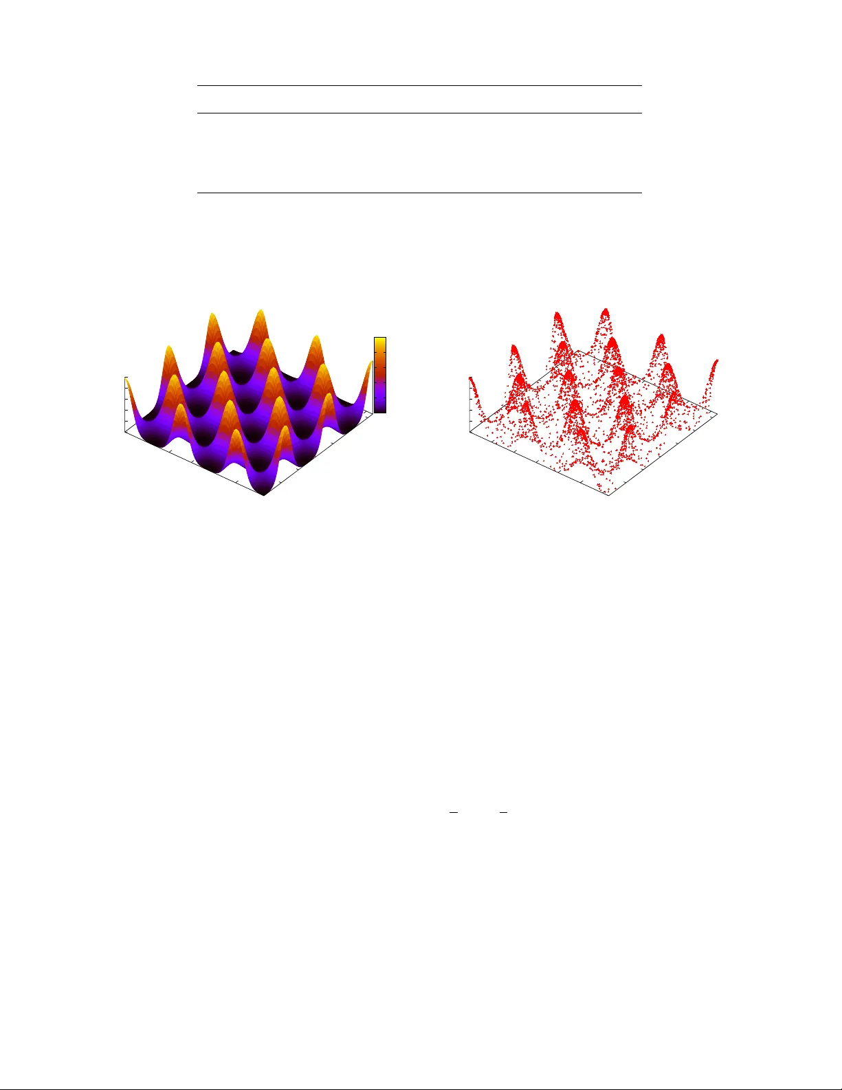
V E R S I O N N OV E M B E R 2 7 , 2 0 1 9 Preprint typeset using L A T E X style openjournal v . 09/06/15 IMPOR T ANCE NESTED SAMPLING AND THE M U L T I N E S T ALGORITHM F . F E RO Z 1 E - M A I L : F . F E RO Z @ M R AO . C A M . AC . U K , M. P . H O B S O N 1 , E . C A M E RO N 2 A N D A . N . P E T T I T T 3 1 A S T R O P H Y S I C S G RO U P , C A V E N D I S H L A B O R A T O RY , J J T H O M S O N A V E N U E , C A M B R I D G E , U K 2 B I G D A TA I N S T I T U T E , L I K A S H I N G C E N T R E F O R H E A LTH I N F O R M A T I O N A N D D I S C OV E RY , U N I V E R S I T Y O F O X F O R D , U K 3 S C H O O L O F M AT H E M A T I C A L S C I E N C E S ( S TA T I S T I C A L S C I E N C E ) , Q U E E N S L A N D U N I V E R S I T Y O F T E C H N O L O G Y ( Q U T ) , B R I S BA N E , A U S T R A L I A Bayesian inference in volv es tw o main computational challenges. First, in estimating the parameters of some model for the data, the posterior distribution may well be highly multi-modal: a regime in which the con ver gence to stationarity of traditional Markov Chain Monte Carlo (MCMC) techniques becomes incredibly slow . Second, in selecting between a set of competing models the necessary estimation of the Bayesian evidence for each is, by definition, a (possibly high-dimensional) inte gration ov er the entire parameter space; again this can be a daunting computational task, although new Monte Carlo (MC) integration algorithms offer solutions of ever increasing efficienc y . Nested sampling (NS) is one such contemporary MC strategy targeted at calculation of the Bayesian evidence, but which also enables posterior inference as a by-product, thereby allo wing simultaneous parameter estimation and model selection. The widely-used M U L T I N E S T algorithm presents a particularly efficient implementation of the NS technique for multi-modal posteriors. In this paper we discuss importance nested sampling (INS), an alternativ e summation of the M U LT I N E S T draws, which can calculate the Bayesian e vidence at up to an order of magnitude higher accurac y than ‘v anilla’ NS with no change in the way M U L T I N E S T explores the parameter space. This is accomplished by treating as a (pseudo- )importance sample the totality of points collected by M U LT I N E S T , including those previously discarded under the constrained likelihood sampling of the NS algorithm. W e apply this technique to se veral challenging test problems and compare the accuracy of Bayesian evidences obtained with INS ag ainst those from vanilla NS. Keyw ords: Bayesian methods, model selection, data analysis, Monte Carlo methods 1. INTR ODUCTION The last two decades in astrophysics and cosmology have seen the arriv al of vast amounts of high quality data. T o facilitate inference regarding the physical processes under in vestigation, Bayesian methods hav e become increasingly important and widely used (see e.g. Trotta 2008 for a re view). In such applications, the process of Bayesian inference may be sensibly divided into tw o distinct categories: parameter estimation and model selection. Parameter estimation is typically achieved via MCMC sampling methods based on the Metropolis-Hastings algorithm and its variants, such as slice and Gibbs sampling (see e.g. Mackay 2003). Unfortunately , these methods can be highly inefficient in exploring multi-modal or degenerate distributions. Moreov er , in order to perform Bayesian model selection (Clyde et al. 2007), estimation of the Bayesian ‘e vidence’, or marginal likelihood, is needed, requiring a multi-dimensional integration over the prior density . Consequently , the computational expense in volved in Bayesian model selection is typically an order of magnitude greater than that for parameter estimation, which has undoubtedly hindered its use in cosmology and astroparticle physics to-date. Nested sampling (NS; Skilling 2004, 2006; Sivia and Skilling 2006) is a contemporary Monte Carlo (MC) method targeted at the efficient calculation of the evidence, yet which allows posterior inference as a by-product, providing a means to carry out simultaneous parameter estimation and model selection (and, where appropriate, model averaging). Feroz and Hobson (2008) and Feroz et al. (2009) have built on the NS framework by introducing the now-popular M U LT I N E S T algorithm, which is especially efficient in sampling from posteriors that may contain multiple modes and/or degeneracies. This technique has already greatly reduced the computational cost of Bayesian parameter estimation and model selection and has successfully been applied to numerous inference problems in astrophysics, cosmology and astroparticle physics (see e.g. Feroz et al. 2009, 2010, 2011 a , b ; Bridges et al. 2009; Graff et al. 2012; White and Feroz 2010; Kipping et al. 2012; Karpenka et al. 2012, 2013; Strege et al. 2013; T eachey and Kipping 2018). In this paper, we discuss importance nested sampling (INS), an alternati ve summation of the draws from M U LT I N E S T ’ s ex- ploration of the model parameter space with the potential to increase its efficienc y in evidence computation by up to a order-of- magnitude. V ersion (v3.0) of M U L T I N E S T , which implements INS in addition to the vanilla NS scheme of previous versions, is av ailable at https://github.com/farhanferoz/MultiNest . The outline of this paper is as follows. W e giv e a brief introduction to Bayesian inference in Sec. 2 and describe nested sampling along with the M U LT I N E S T algorithm in Sec. 3. The INS technique is discussed in Sec. 4 and is applied to several test problems in Sec. 5. W e summarize our findings in Sec. 6. Finally , in Appendix A we discuss the relationship between INS and other contemporary MC schemes, in Appendix B we gi ve a detailed account of the con vergence properties of INS within the M U LT I N E S T algorithm, and in Appendix C we present a brief measure-theoretic commentary on vanilla NS. 2. BA YESIAN INFERENCE Bayesian inference provides a principled approach to the inference of a set of parameters, Θ , in a model (or hypothesis), H , for data, D . Bayes’ theorem states that Pr( Θ | D , H ) = Pr( D | Θ , H ) Pr( Θ | H ) Pr( D | H ) , (1) 2 L 1 L 2 L 3 L 4 . . . . (a) . L 1 L 2 L 3 L 4 X 1 . . . . X 2 X 3 X 4 (b) F I G . 1 . — Cartoon illustrating (a) the posterior of a two dimensional problem; and (b) the transformed L ( X ) function where the prior volumes, X i , are associated with each likelihood, L i . where Pr( Θ | D , H ) ≡ P ( Θ | D ) is the posterior probability density of the model parameters, Pr( D | Θ , H ) ≡ L ( Θ ) the likelihood of the data, and Pr( Θ | H ) ≡ π ( Θ ) the parameter prior . The final term, Pr( D | H ) ≡ Z (the Bayesian evidence), represents the factor required to normalize the posterior ov er the domain of Θ given by: Z = Z Ω Θ L ( Θ ) π ( Θ ) d Θ . (2) Being independent of the parameters, ho wever , this factor can be ignored in parameter inference problems which can be approx- imated by taking samples from the unnormalized posterior only , using standard MCMC methods (for instance). Model selection between two competing models, H 0 and H 1 , can be achiev ed by comparing their respective posterior proba- bilities giv en the observed dataset as follo ws: R = Pr( H 1 | D ) Pr( H 0 | D ) = Pr( D | H 1 ) Pr( H 1 ) Pr( D | H 0 ) Pr( H 0 ) = Z 1 Z 0 Pr( H 1 ) Pr( H 0 ) . (3) Here Pr( H 1 ) / Pr( H 0 ) is the prior probability ratio for the two models, which can often be set to unity in situations where there is no strong a priori reason for preferring one model over the other , but occasionally requires further consideration (as in the Prosecutor’ s Fallacy; see also Feroz et al. 2008, 2009 for key astrophysical examples). It can be seen from Eq. (3) that the Bayesian evidence thus plays a central role in Bayesian model selection. As the average of the likelihood over the prior , the evidence is generally larger for a model if more of its parameter space is likely and smaller for a model with lar ge areas in its parameter space having low likelihood values, ev en if the lik elihood function is sharply peaked. Thus, the evidence may be seen both as penalizing ‘fine tuning’ of a model against the observed data and as an automatic implementation of Occam’ s Razor . 3. NESTED SAMPLING AND THE M U LTI N E S T ALGORITHM Nested sampling estimates the Bayesian evidence by transforming the multi-dimensional evidence integral ov er the prior den- sity into a one-dimensional inte gral over an in verse survi val function (with respect to prior mass) for the likelihood itself. This is accomplished by considering the surviv al function, X ( λ ) , for L ( Θ ) , dubbed “the prior volume” here; namely , X ( λ ) = Z { Θ : L ( Θ ) >λ } π ( Θ ) d Θ , (4) where the integral extends over the region(s) of parameter space contained within the iso-likelihood contour , L ( Θ ) = λ . Re- calling that the expectation v alue of a non-ne gativ e random v ariable may be reco vered by inte gration over its survi val function (a result evident from inte gration by parts) we hav e (unconditionally): Z = Z ∞ 0 X ( λ ) dλ. (5) When L ( X ) , the in verse of X ( λ ) , exists (i.e., when L ( Θ ) is a continuous function with connected support; Chopin and Robert 2010) the evidence inte gral may thus be further rearranged as: Z = Z 1 0 L ( X ) dX . (6) 3 Indeed, if L ( X ) were known exactly (and Riemann integrable 1 ), by ev aluating the likelihoods, L i = L ( X i ) , for a deterministic sequence of X values, 0 < X N < · · · < X 2 < X 1 < X 0 = 1 , (7) as shown schematically in Fig. 1, the e vidence could in principle be approximated numerically using only standard quadrature methods as follows: Z ≈ ˆ Z = N X i =1 L i w i , (8) where the weights, w i , for the simple trapezium rule are giv en by w i = 1 2 ( X i − 1 − X i +1 ) . W ith L ( X ) typically unknown, howe ver , we must turn to MC methods for the probabilistic association of prior v olumes, X i , with likelihood contours, L i = L ( X i ) , in our computational evidence estimation. 3.1. Evidence estimation Under the default nested sampling algorithm the summation in Eq. (8) is performed as follo ws. First N live ‘liv e’ points are drawn from the prior , π ( Θ ) , and the initial prior volume, X 0 , is set to unity . At each subsequent iteration, i , the point with lowest likelihood v alue, L i , is removed from the liv e point set and replaced by another point drawn from the prior under the constraint that its likelihood is higher than L i . The prior v olume contained within this region at the i th iteration, is thus a random variable distrib uted as X i = t i X i − 1 , where t i follows the distrib ution for the largest of N live samples drawn uniformly from the interval [0 , 1] (i.e., Pr( t ) = N live t N live − 1 ). This sampling process is repeated until (effecti vely) the entire prior volume has been trav ersed; the liv e particles moving through nested shells of constrained likelihood as the prior volume is steadily reduced. The mean and standard deviation of log t , which governs the geometrical e xploration of the prior volume, are: E [log t ] = − 1 / N live , σ [log t ] = 1 / N live . (9) Since each draw of log t i is independent here, after i iterations the prior volume will shrink down as log X i ≈ − ( i ± √ i ) / N live . Thus, one may take X i ≈ exp( − i/ N live ) . 3.2. Stopping criterion The NS algorithm should terminate when the expected evidence contribution from the current set of live points is less than a user-defined tolerance. This expected remaining contribution can be estimated (cautiously) as ∆ Z i = L max X i , where L max is the maximum likelihood value amongst the current set of liv e points (with X i the expected value of remaining prior volume, as before). 3.3. P osterior infer ences Although the NS algorithm is designed specifically to estimate the Bayesian evidence, inferences from the posterior distrib ution can be easily obtained using the final liv e points and the full sequence of discarded points from the NS process, i.e., the points with the lowest lik elihood value at each iteration of the algorithm. Each such point is simply assigned the importance weight, p i = L i w i P j L j w j = L i w i ˆ Z , (10) from which sample-based estimates for the ke y posterior parameter summaries (e.g. means, standard deviations, covariances and so on) may be computed 2 . (As a self-normalizing importance sampling estimator the asymptotic variance of these moments is of course dependent upon both the similarity between the NS path and the tar get and the accuracy of ˆ Z itself; cf. Hesterberg 1995.) Readers unfamiliar with importance sampling (IS) ideas may refer to Liu (2008) for an insightful ov erview of this topic and its application to diverse branches of modern science (including statistical physics, cell biology , target tracking, and genetic analysis). 3.4. Practical implementations of nested sampling The main challenge in implementing the computational NS algorithm is to draw unbiased samples efficiently from the likelihood-constrained prior . John Skilling, originally proposed to use the Marko v Chain Monte Carlo (MCMC) method for this purpose (Skilling 2004, 2006; Sivia and Skilling 2006). One such implementation (V eitch and V ecchio 2010), with specific proposal distributions for the MCMC step, has been used successi vely in gra vitational wav e searches. In astrophysics in particular, rejection sampling schemes hav e been successfully employed to draw samples from the likelihood- constrained prior . It was first proposed in the C O S M O N E S T package (Mukherjee et al. 2006) through the use of ellipsoidal rejection sampling scheme and was shown to work very well for uni-modal posterior distributions. This method was improv ed upon in C O S M O C L U S T package (Sha w et al. 2007) through the use of a clustering scheme to deal with multi-modal distrib utions. M U LT I N E S T was then proposed with several innov ations to make ellipsoidal rejection sampling more rob ust in dealing with multi-modal distributions. Other methods employing ellipoidal rejection sampling scheme within Nested Sampling framew ork include the D I A M O N D S (Corsaro and De Ridder 2014) and D Y N E S T Y (Speagle 2019) packages. 1 W e give a brief measure-theoretic formulation of NS in Appendix C. 2 Some relev ant commentary on this aspect of NS with regard to Lemma 1 of Chopin and Robert (2010) appears in Appendix C. 4 (a) (b) F I G . 2 . — Illustrations of the ellipsoidal decompositions returned by M U LT I N E S T . The points given as input are overlaid on the resulting ellipsoids. Here 1000 points were sampled uniformly from: (a) two non-intersecting ellipsoids; and (b) a torus. One particular problem with rejection sampling schemes is the exponential reduction in sampling efficiency with increasing dimensionality of the problem. In order to address this issue, a slice sampling method has been employed to draw unbiased samples efficiently from the lik elihood-constrained prior in the P O L Y C H O R D (Handley et al. 2015a,b) package. Another algorithm to increase the efficienc y of Nested Sampling through the variable number of liv e points is the “Dynamic Nested Sampling” method (Higson et al. 2018) which has been used in the D Y N E S T Y (Speagle 2019) package. 3.5. M U LT I N E S T algorithm The M U LT I N E S T algorithm (Feroz and Hobson 2008; Feroz et al. 2009) addresses this problem of drawing unbiased samples from the likelihood-constrained prior, through an ellipsoidal rejection sampling scheme. At each iteration, i , the full set of N live liv e points is enclosed within a set of (possibly overlapping) ellipsoids and the desired replacement point sought from within their union. The ellipsoidal decomposition of the liv e point set is performed through an expectation-minimisation algorithm such that the sum of volumes of the ellipsoids is minimised with the additional constraint that the total volume enclosed by the ellipsoids is at least X i /f . Again X i ≈ exp( − i/ N live ) is the expected prior v olume, while 0 < f ≤ 1 is a user defined value for the target efficienc y (the ratio of points accepted to points sampled). Thus, f is analogous to the (in verse of the) “enlargement factor” introduced by Mukherjee et al. (2006) into their pioneering ellipsoid-based NS code; the larger the target f the faster the algorithm runs, b ut the greater the chance of some ellipsoids failing to cover the full L > L i volume (biasing the v anilla NS estimates, though not necessarily the INS estimates, as we discuss later). The M U LT I N E S T ellipsoidal decomposition algorithm thus allows substantial flexibility in the geometry of its posterior e xplo- ration; with bent and/or irregularly-shaped posterior modes typically broken into a relati vely lar ge number of small ‘overlapping’ ellipsoids and smooth, near-Gaussian posterior modes kept whole (or broken into relativ ely few ellipsoids), as shown in Fig. 2. It thereby automatically accommodates elongated, curving degeneracies while maintaining high ef ficiency for simpler problems. M U LT I N E S T also specifically enables the identification of distinct modes by isolating non-overlapping subsets of the ellipsoidal decomposition; so identified, these distinct modes can then be ev olved independently . Once the ellipsoidal bounds ha ve been created at a gi ven iteration of the M U LT I N E S T algorithm a new point is drawn uniformly from the union of these ellipsoids as follows. If there are L ellipsoids at iteration i , a particular ellipsoid is chosen with probability p l giv en as: p l = V l /V tot , (11) where V tot = P L l =1 V l , from which a single point is then drawn uniformly and checked against the constraint L > L i . If satisfied the point is accepted with probability 1 /q , where q is the number of ellipsoids the new point lies in (in order to take into account the possibility of non-empty intersections), otherwise it is rejected (but sav ed for INS summation) and the process is repeated with a new random choice of ellipsoid. In higher dimensions, most of the volume of an ellipsoid lies in its outer shells and therefore any overshoot of the ellipsoidal decomposition relativ e to the true iso-likelihood surface can result in a marked drop in sampling efficiency . In order to maintain the sampling efficiency for such high dimensional problems, M U LT I N E S T can also operate in a ‘constant ef ficiency mode’. In this mode, the total volume enclosed by the ellipsoids is no longer linked with the expected prior volume X i by requiring the total ellipsoidal volume to be at least X i /f , instead the total volume enclosed by the union of ellipsoids is adjusted such that the sampling efficienc y is as close to the user defined target efficiency f as possible while keeping every liv e point enclosed in at least one ellipsoid. Despite the increased chance of the fitted ellipsoids encroaching within the constrained-likelihood volume (i.e., missing regions of parameter space for which L > L i ), past experience has shown (e.g. Feroz et al. 2009) this constant efficienc y mode may ne vertheless produce reasonably accurate posterior distrib utions for parameter estimation purposes. The vanilla NS evidence values, howe ver , cannot be relied upon in this mode, with the e xpectation being a systematic o ver -estimation of the model evidence. Interestingly , the same is not strictly true of the INS evidence estimates, which use the NS technique only for posterior exploration (not e vidence summation); though we will note later some important cav eats for its error estimation. 5 In the rest of this paper , we refer to the mode in which M U LT I N E S T links the volume of the ellipsoidal decomposition with the expected prior volume as its ‘default’ mode, and we specifically highlight instances where ‘constant efficiency mode’ has been trialled. 4. IMPOR T ANCE NESTED SAMPLING Though highly efficient in its approximation to the iso-likelihood contour bounding the liv e particle set at each iteration, the ellipsoidal rejection sampling scheme used by M U LT I N E S T ultimately discards a significant pool of sampled points failing to satisfy the NS constraint, L > L i , for which the likelihood has ne vertheless been e valuated at some computational cost. In order to redress this final inefficiency the technique of importance nested sampling (INS) has recently been proposed by Cameron and Pettitt (2013) as an alternativ e summation for the Bayesian evidence in this context. In particular, INS uses all the points drawn by M U LT I N E S T , or any other ellipsoidal rejection sampling algorithm, at each iteration regardless of whether they satisfy the constraint L > L i or not. The relationship of INS to existing MC schemes is summarised in Appendix A. 4.1. Pseudo-importance sampling density One begins by defining the follo wing pseudo-importance sampling density: g ( Θ ) = 1 N tot N iter X i =1 n i E i ( Θ ) V tot ,i , (12) where N iter is the total number of iterations (ellipsoidal decompositions) performed by M U LT I N E S T , n i the number of points collected at the i th iteration (with total, N tot = P N iter i =1 n i ), V tot ,i the total volume enclosed in the union of ellipsoids at the i th iteration, and E i ( Θ ) an indicator function returning 1 when Θ lies in the i th ellipsoidal decomposition and 0 otherwise. W e call g ( Θ ) here a pseudo -importance sampling density since it is of course defined only a posteriori to our sampling from it, with the consequence that all Θ ∼ E j >i ( Θ ) are to some (ideally negligible) extent dependent on all previous Θ ∼ E j ≤ i ( Θ ) (some important implications of which we discuss in Sec. 4.3 belo w). The heritage of this technique lies with the rev erse logistic regression strategy of Geyer (1994) and the “biased sampling” framew ork of V ardi (1985). Another term that has been used in place of pseudo-importance sampling is “recycling of past dra ws” (e.g. Cornuet et al. 2012). If at each iteration, the ellipsoidal decomposition w ould consis t of only one ellipsoid then V tot ,i is simply the geometric volume of the ellipsoid at iteration i . M U LT I N E S T , howev er , may enclose its liv e points in a set of possibly overlapping ellipsoids. An analytical expression for calculating the volume in the overlapped region of ellipsoids is not av ailable and therefore we estimate the volume occupied by the union of ellipsoids through the following MC method. Whenev er an ellipsoidal decomposition is constructed, we draw M points ( Θ 0 m , m = 1 , 2 , . . . , M ) from it as follows: for each draw we first pick an ellipsoid with probability V l / P L l =1 V l , where V l are the v olumes of the L ellipsoids in the decomposition; a point Θ 0 m is then dra wn uniformly from the chosen ellipsoid and we calculate, q m , the number of ellipsoids it lies in. The volume in the union of ellipsoids is then: V tot ≈ ˆ V tot = M P M m =1 q m L X l =1 V l . (13) W e note that this Monte Carlo procedure does not require an y e valuations of the likelihood function, and thus is not computation- ally demanding. 4.2. Evidence estimation and posterior samples As an alternativ e to the canonical NS summation given by Eq. (8) the Bayesian evidence can instead be estimated with reference to the abov e pseudo-importance sampling density as: ˆ Z = 1 N tot N tot X k =1 L ( Θ k ) π ( Θ k ) g ( Θ k ) . (14) Moreov er, each one of the N tot points collected by M U L T I N E S T can be assigned the following estimator of its posterior proba- bility density: P ( Θ ) = L ( Θ ) π ( Θ ) N tot g ( Θ ) . (15) Since the importance nested sampling scheme does not rely on the ellipsoidal decomposition fully enclosing the region(s) satis- fying the constraint L > L i , it can also achiev e accurate evidence estimates and posterior summaries from sampling done in the constant efficiency mode of M U L T I N E S T . 3 Howe ver , as we discuss shortly , the utility of this feature is often limited by ensuing difficulties in the estimation of uncertainty for such constant ef ficiency mode evidence estimates. From a computational perspective we note that in a na ¨ ıve application of this scheme it will be necessary to store N tot points, Θ k , along with the likelihood, L ( Θ k ) , and prior probability , π ( Θ k ) , for each, as well as all relev ant information describing the ellipsoidal decompositions (centroids, eigen-values and eigen-vectors) at each iteration. Even with a Cholesky factorization of 3 The reasons for this are described in detail in Appendix B; but in brief we note that like ‘ordinary’ importance sampling the only fundamental constraint on the g ( Θ ) of the INS scheme is that its support enclose that of the posterior, which we ensure by drawing our first set of points from the prior support itself, E 1 ( Θ ) = 1 whenever π ( Θ ) > 0 . 6 the eigen-vectors, storing the latter may easily result in excessiv e memory requirements. Howe ver , since in the M U LT I N E S T al- gorithm the prior v olume, and consequently the volume occupied by the bounding ellipsoids, shrinks at each subsequent iteration one can confidently assume E i ( Θ ) = 1 for all points dra wn at iterations j > i . At a gi ven iteration then, one needs only to check if points collected from previous iterations lie in the current ellipsoidal decomposition and add the contribution to g ( Θ ) coming from the current iteration as given in Eq. (12). This results in an enormous reduction in memory requirements as information about the ellipsoidal decomposition from previous iterations no longer needs to be stored. At each iteration, M U LT I N E S T draws points from the ellipsoidal decomposition, but in order to take account of the volume in the overlaps between ellipsoids, each point is accepted only with probability 1 /q where q is the number of ellipsoids in which the given point lies. Rather than discarding all these rejected points, which would be wasteful, we include them by dividing the importance sampling weights as giv en in Eq. (12), in three components: g ( Θ ) = g 1 ( Θ ) + g 2 ( Θ ) + g 3 ( Θ ) . (16) Assuming that the point Θ was drawn at iteration i , g 1 , g 2 and g 3 are the contributions to importance weight for Θ coming from iteration i , iterations before i and iterations after i respectiv ely . Thus, g 1 is calculated as follows: g 1 ( Θ ) = q n i N tot V tot ,i , (17) where q is the number of ellipsoids at iteration i in which point Θ lies, while g 2 is calculated as follows: g 2 ( Θ ) = 1 N tot i − 1 X j =1 n j V tot , j , (18) where V tot ,j is volume occupied by the union of ellipsoids at iteration j as giv en in Eq. (13). Here we hav e assumed that ellipsoids shrink at subsequent iterations and therefore points drawn at iteration i lie inside the ellipsoidal decompositions of previous iterations as discussed earlier . Finally , g 3 is calculated as follows: g 3 ( Θ ) = 1 N tot n iter X j = i +1 n j E j ( Θ ) V tot ,j . (19) 4.3. Evidence err or estimation As discussed by Skilling (2004) (and by Feroz and Hobson 2008; Feroz et al. 2009 for the specific case of M U LT I N E S T ) repeated summation of the NS draws under random sampling of the associated X i (gov erned by t i ; cf. Sec. 3) allo ws one to estimate the error on the NS evidence approximation from just a single run (whereas man y other MC integration techniques, such as thermodynamic integration, require repeat runs to achieve this). Provided that the parameter space has been explored with sufficient thoroughness (i.e., the N live point set has ev olved through all the significant posterior modes), the reliability of this evidence estimate was demonstrated in Feroz and Hobson (2008). Importantly , such a single run error estimate can also be calculated for the INS scheme as described below . Under ordinary (as opposed to pseudo-) importance sampling the unbiased estimator for the asymptotic variance of the evidence estimate here, d V ar[ ˆ Z ] , would be gi ven as follows: d V ar[ ˆ Z ] = 1 N tot ( N tot − 1) N tot X k =1  L ( Θ k ) π ( Θ k ) g ( Θ k ) − ˆ Z  2 , (20) with ˆ Z giv en by Eq. (14). W ith the draws from M U L T I N E S T representing our a posteriori constructed g ( Θ ) not in fact an independent, identically distributed sequence from this pseudo-importance sampling function, the abo ve uncertainty estimate is, unfortunately , not strictly applicable here. In particular , with the placement of subsequent ellipses, E j >i , dependent on the position of the liv e particles drawn up to the present step, i , so too are the subsequently drawn Θ j >i . Howe ver , when M U LT I N E S T is run in its default mode, such that we strongly govern the maximum rate at which the volume of the successive E i can shrink we can be confident that our sampling becomes e ver more nearly independent and that the dominant variance component is indeed gi ven in Eq. (20). Our reasoning behind this is explained in detail in Appendix B. On the other hand, when M U L T I N E S T is being run in ‘constant efficienc y mode’ we recommended for the user to check (via repeat simulation) that the INS evidence is stable (with respect to its error estimate) for reasonable variation in N live and/or f . 5. APPLICA TIONS In this section we apply the M U LT I N E S T algorithm with INS described abov e to three test problems to demonstrate that it indeed calculates the Bayesian evidence much more accurately than vanilla NS. These test examples are chosen to have features that resemble those that can occur in real inference problems in astro- and particle physics. 5.1. T est problem 1: Gaussian shells likelihood 7 -6 -4 -2 0 2 4 6 -6 -4 -2 0 2 4 6 0 1 2 3 4 L x y L 0 0.5 1 1.5 2 2.5 3 3.5 4 (a) -6 -4 -2 0 2 4 6 -6 -4 -2 0 2 4 6 0 1 2 3 4 L x y L (b) F I G . 3 . — T est problem 1: (a) two-dimensional plot of the likelihood function defined in Eqs. (21) and (22); (b) dots denoting the points with the lowest likelihood at successi ve iterations of the M U LT I N E S T algorithm. D N live f N like default N like ceff 2 300 0 . 30 4 , 581 3 , 871 5 300 0 . 30 8 , 922 7 , 882 10 300 0 . 05 73 , 342 76 , 255 20 300 0 . 05 219 , 145 163 , 234 30 500 0 . 05 604 , 906 548 , 501 50 500 0 . 01 10 , 531 , 223 5 , 290 , 550 T A B L E 1 D I M E N S I O NA L I T Y ( D ) O F P RO B L E M , N U M B E R O F L I V E P O I N T S ( N live ) , TAR G E T E FFI C I E N C Y ( f ) A N D T H E T OTA L N U M B E R O F L I K E L I H O O D E V A L U A T I O N S ( N like ) I N D E FAU LT A N D C O N S TA N T E FFI C I E N C Y ( C E FF ) M O D E S O F M U LT I N E S T F O R T E S T P RO B L E M 1 , D I S C U S S E D I N S E C . 5 . 1 . In this section, we apply M U L T I N E S T with and without INS to sample from a posterior containing multiple modes with pronounced (curving) degeneracies in relativ ely high dimensions. Our test problem here is the same one used in Allanach and Lester (2008); Feroz and Hobson (2008); Feroz et al. (2009). The likelihood function of this problem is defined as, L ( θ ) = circ( θ ; c 1 , r 1 , w 1 ) + circ( θ ; c 2 , r 2 , w 2 ) , (21) where circ( θ ; c , r, w ) = 1 √ 2 π w 2 exp  − ( | θ − c | − r ) 2 2 w 2  . (22) In two dimensions, this distribution represents two well separated rings, centred on the points c 1 and c 2 respectiv ely , each of radius r and with a Gaussian radial profile of width w (see Fig. 3). W e inv estigate the above distribution up to a 50 -dimensional parameter space θ . In all cases, the centres of the two rings are separated by 7 units in the parameter space, and we take w 1 = w 2 = 0 . 1 and r 1 = r 2 = 2 . W e make r 1 and r 2 equal, since in higher dimensions any slight dif ference between these tw o v alues w ould result in a vast difference between the volumes occupied by the rings and consequently the ring with the smaller r value w ould occupy a v anishingly small fraction of the total probability volume, making its detection almost impossible. It should also be noted that setting w = 0 . 1 means the rings have an extremely narrow Gaussian profile. W e impose uniform priors U ( − 6 , 6) on all the parameters. For the two-dimensional case, with the parameters described abov e, the likelihood is shown in Fig. 3. T able 1 lists the total number of li ve points ( N live ) and tar get ef ficiency ( f ) used and the total number of likelihood e valuations ( N like ) performed by M U L T I N E S T in default and constant efficiency (cef f) modes. The volume of the parameter space increases exponentially with the dimensionality D , therefore we need to increase N live and/or decrease f with D , in order to get accurate estimates of log( Z ) . The true and estimated values of log( Z ) are listed in T able 2. It can be seen from T able 2 that log( ˆ Z ) v alues obtained by M U LTI N E S T with and without INS and in both default and constant efficienc y modes are consistent with the true log( Z ) for D ≤ 20 , the only exception being the log( ˆ Z ) from constant efficiency mode with INS which is ∼ 6 σ away from the analytical log( Z ) . W e attribute this to the heightened potential for underestimation of the INS uncertainties in constant ef ficiency mode discussed in Sec. 4 and Appendix B. For D ≥ 30 howe ver , the log ( ˆ Z ) values obtained by M U LT I N E S T without INS start to become inaccurate, with constant ef ficiency mode again giving more inaccurate results as expected. These inaccuracies are caused by inadequate numbers of live points used to cover the region satisfying the constraint L > L i at each iteration i . Howe ver , with the same values for N live and f , and indeed with the same set of points, 8 Analytical M U LTI N E S T without INS M U LTI N E S T with INS D default cef f default cef f 2 − 1 . 75 − 1 . 61 ± 0 . 09 − 1 . 71 ± 0 . 09 − 1 . 72 ± 0 . 02 − 1 . 69 ± 0 . 02 5 − 5 . 67 − 5 . 42 ± 0 . 15 − 5 . 78 ± 0 . 15 − 5 . 67 ± 0 . 03 − 5 . 87 ± 0 . 03 10 − 14 . 59 − 14 . 55 ± 0 . 23 − 14 . 83 ± 0 . 23 − 14 . 60 ± 0 . 03 − 14 . 58 ± 0 . 03 20 − 36 . 09 − 35 . 90 ± 0 . 35 − 35 . 99 ± 0 . 35 − 36 . 11 ± 0 . 03 − 36 . 06 ± 0 . 03 30 − 60 . 13 − 59 . 72 ± 0 . 35 − 59 . 43 ± 0 . 34 − 60 . 09 ± 0 . 02 − 59 . 90 ± 0 . 02 50 − 112 . 42 − 110 . 69 ± 0 . 47 − 108 . 96 ± 0 . 46 − 112 . 37 ± 0 . 01 − 112 . 18 ± 0 . 01 T A B L E 2 T H E T RU E A N D E S T I M ATE D log( Z ) F O R T E S T P RO B L E M 1 , D I S C U S S E D I N S E C . 5 . 1 , A S A F U N C T I O N O F T H E D I M E N S I O N S D O F T H E PA R A M E T E R S PAC E , U S I N G M U LTI N E S T W I T H A N D W I T H O U T I N S A N D I N I T S D E FAU LT A N D C O N S TA N T E FFI C I E N C Y M O D E S . 0 5 10 15 20 25 30 0 5 10 15 20 25 30 0 50 100 150 200 250 log L x y log L 0 50 100 150 200 250 (a) 0 5 10 15 20 25 30 0 5 10 15 20 25 30 0 50 100 150 200 250 log L x y log L (b) F I G . 4 . — T est problem 2: (a) two-dimensional plot of the likelihood function defined in Eq. 23; (b) dots denoting the points with the lowest likelihood at successiv e iterations of the M U LTI N E S T algorithm. INS returns log ( ˆ Z ) values which are consistent with the true log( Z ) in default M U LT I N E S T mode and off by at most ∼ 0 . 2 in the constant ef ficiency mode. The error estimate on log ( ˆ Z ) from INS in the constant efficienc y mode might indicate that log ( ˆ Z ) has a large bias but as discussed in Sec. 4.3, these error estimates are reliable only when the importance sampling distribution is guaranteed to gi ve non-vanishing probabilities for all re gions of parameter space where posterior distribution has a non-vanishing probability as well. This is much more difficult to accomplish in a 50 D parameter space. In addition to this, the approximations we hav e made to calculate the v olume in the overlapped region of ellipsoids are e xpected to be less accurate in higher dimensions. Therefore, it is very encouraging that INS can obtain log( Z ) to within 0 . 2 units for a v ery challenging 50 D problem with just 500 liv e points. W e should also notice the number of likelihood e valuations in constant ef ficiency mode starts to become significantly smaller than in the default mode for D ≥ 20 . 5.2. T est problem 2: eg g-box likelihood W e now demonstrate the application of M U LT I N E S T to a highly multimodal two-dimensional problem, for which the likelihood resembles an egg-box. The un-normalized likelihood is defined as: L ( x, y ) = exp  h 2 + cos  x 2  cos  y 2 i 5  , (23) and we assume a uniform prior U (0 , 10 π ) for both x and y . A plot of the log-likelihood is shown in Fig. 4 and the prior ranges are chosen such that some of the modes are truncated, making it a challenging problem for identifying all the modes as well as to calculate the e vidence accurately . The true value of the log-evidence is log Z = 235 . 856 , obtained by numerical integration on a very fine grid, which is feasible for this simple two-dimensional example. It was sho wn in Feroz et al. (2009) that M U L T I N E S T can e xplore the parameter space of this problem ef ficiently , and also calculate the evidence accurately . Here we demonstrate the accuracy of the evidence obtained with M U LT I N E S T using the INS summation. For low-dimensional problems, results obtained with the constant efficienc y mode of M U L T I N E S T agree very well with the ones obtained with the default mode, we therefore only discuss the default mode results in this section. W e use 1000 live points with target efficiency f = 0 . 5 . The results obtained with M U LT I N E S T are illustrated in Fig. 4, in which the dots show the points with the lowest likelihood at successive iterations of the nested sampling process. M U LT I N E S T required ∼ 20 , 000 likelihood e valuations and obtained log( ˆ Z ) = 235 . 837 ± 0 . 008 ( 235 . 848 ± 0 . 078 ) with (without) INS, which 9 θ 1 θ 2 0 0.2 0.4 0.6 0.8 1 0 0.2 0.4 0.6 0.8 1 (a) θ 1 θ 2 0 0.2 0.4 0.6 0.8 1 0 0.2 0.4 0.6 0.8 1 (b) F I G . 5 . — T est problem 3: Marginalized posterior distribution in the first 2 dimensions of the 16D Gaussian mixture model discussed in Sec. 5.3. Panel (a) shows the analytical distrib ution while panel (b) shows the distribution obtained from M U LT I N E S T . The contours represent the 68% and 95% Bayesian credible regions. compares fa vourably with the true value giv en abov e. In each case, the random number seed w as the same, so the points sampled by M U LT I N E S T were identical with and without INS. In order to check if the error estimates on log ( ˆ Z ) are accurate, we ran 10 instances of M U LT I N E S T in both cases, each with a different seed and found the mean and standard deviation of log ( ˆ Z ) to be 235 . 835 ± 0 . 009 ( 235 . 839 ± 0 . 063 ) with (without) INS. In both cases, the standard error agrees with the error estimate from just a single run. There is, howe ver , some indication of bias in the log ( ˆ Z ) v alue ev aluated with INS, which lies ∼ 2 σ away from the true value. This is most likely due to the approximations used in calculating the volume in the ov erlapped region of ellipsoids, as discussed in Sec. 4. Nonetheless, the absolute value of the bias is very lo w ( ∼ 0 . 02 ), particularly compared with the accuracy ( ∼ 0 . 5 ) to which log-evidence v alues are usually required in practical applications. 5.3. T est problem 3: 16D Gaussian mixture model Our next test problem is the same as test problem 4 in W einberg et al. (2013) which is a mixture model of four randomly- oriented Gaussian distrib utions with their centers uniformly selected from the hypercube [0 . 5 − 2 σ, 0 . 5 + 2 σ ] D with D being the dimensionality of the problem and the variance σ 2 of all four Gaussians is set to 0 . 003 . W eights of the Gaussians are distributed according to a Dirichlet distribution with shape parameter α = 1 . W e impose uniform priors U (0 , 1) on all the parameters. The analytical posterior distribution for this problem, mar ginalized in the first two dimensions is sho wn in Fig. 5(a). The analytical value of log( Z ) for this problem is 0 , regardless of D . W e set D = 16 and used 300 liv e points with target efficienc y f = 0 . 05 . The marginalized posterior distribution in the first two dimensions, obtained with the default mode of M U LT I N E S T with INS is shown in Fig. 5(b). The posterior distribution obtained from the constant efficienc y mode is identical to the one obtained from the default and therefore we do not show it. In the default mode M U LT I N E S T performed 208 , 978 likelihood ev aluations and returned log( ˆ Z ) = − 0 . 03 ± 0 . 01 ( 0 . 39 ± 0 . 27 ) with (without) INS. In the constant efficiency mode, 158 , 219 likelihood e valuations were performed and log( ˆ Z ) = 0 . 21 ± 0 . 01 ( 0 . 25 ± 0 . 27 ) with (without) INS. 5.4. T est problem 4: 20D Gaussian-LogGamma mixture model Our final test problem is the same as test problem 2 in Beaujean and Caldwell (2013), in which the likelihood is a mixture model consisting of four identical modes, each of which is a product of an equal number of Gaussian and LogGamma 1D distributions, centred at θ 1 = ± 10 , θ 2 = ± 10 , θ 3 = θ 4 = · · · = θ D = 0 in the hypercube θ ∈ [ − 30 , 30] D , where D is the (even) dimensionality of the parameter space. Each Gaussian distribution has unit variance. The LogGamma distribution is asymmetric and heavy-tailed; its scale and shape parameters are both set to unity . W e impose uniform priors U ( − 30 , 30) on all the parameters. The analytical marginalised posterior distribution in the subspace ( θ 1 , θ 2 ) is shown in Fig. 6(a). W e set D = 20 , for which the analytical v alue of the log-evidence is log( Z ) = log (60 − 20 ) = − 81 . 887 . T o be consistent with test problem 3, which is of similar dimensionality , we again used 300 live points with a target efficiency f = 0 . 05 (note these v alues differ from those used in Beaujean and Caldwell (2013), who set N live = 1000 and f = 0 . 3 in the standard vanilla NS version of M U LT I N E S T ). The mar ginalized posterior in the first two dimensions, obtained in the default mode of M U LT I N E S T with INS is shown in Fig. 6(b), and is identical to the corresponding analytical distribution, recov ering all four modes with very close to equal weights. The posterior distribution obtained from the constant ef ficiency mode is identical to the one obtained from the default and therefore we do not show it. In the default mode M U LT I N E S T performed 2,786,538 likelihood ev aluations and returned log ( ˆ Z ) = − 81 . 958 ± 0 . 008 ( − 78 . 836 ± 0 . 398 ) with (without) INS. In both cases, we see that, for this more challenging problem containing multi-dimensional heavy-tailed distributions, the log-evidence estimates are substantially biased, with each being ∼ 8 σ from the true value. Nonetheless, we note that the estimate using INS is much more accurate than that obtained with vanilla NS, and differs from the true value by only ∼ 0 . 1 units, which is much smaller than the accuracy required in most practical applications. As one might expect, howe ver , the log-evidence estimates obtained in constant 10 (a) (b) F I G . 6 . — T est problem 4: Marginalized posterior distribution in the first 2 dimensions of the 20D Gaussian-LogGamma mixture model discussed in Sec. 5.4. Panel (a) shows the analytical distribution while panel (b) shows the distribution obtained from M U LT I N E S T . The contours represent the 68% and 95% Bayesian credible regions. efficienc y mode are somewhat poorer and show a significant bias. In this mode, 297 , 513 likelihood e valuations were performed and log( ˆ Z ) = − 82 . 383 ± 0 . 010 ( − 71 . 635 ± 0 . 376 ) with (without) INS. 6. SUMMAR Y AND DISCUSSION W ith the av ailability of vast amounts of high quality data, statistical inference is increasingly playing an important role in cosmology and astroparticle physics. MCMC techniques and more recently algorithms based on nested sampling have been employed successfully in a variety of different areas. The M U LT I N E S T algorithm in particular has recei ved much attention in astrophysics, cosmology and particle physics owing to its ability to efficiently explore challenging multi-modal distributions as well as to calculate the Bayesian evidence. In this paper we hav e discussed further dev elopment of the M U LT I N E S T algorithm, based on the implementation of the INS scheme recently proposed by Cameron and Pettitt (2013). INS requires no change in the way M U LT I N E S T explores the parameter space, but can calculate the Bayesian evidence at up to an order-of-magnitude higher accuracy than vanilla nested sampling. Moreov er, INS also provides a means to obtain reasonably accurate e vidence estimates from the constant ef ficiency mode of M U LT I N E S T . This is particularly important, as the constant efficienc y mode enables M U LT I N E S T to explore higher -dimensional spaces (up to ∼ 50 D ) much more efficiently than the default mode. Higher evidence accurac y from INS could potentially allow users to use fe wer liv e points N live or higher target efficiency f to achiev e the same lev el of accuracy as v anilla nested sampling, and therefore to speed-up the analysis by se veral factors. W e recommend that users should alw ays check that their posterior distributions are stable with reasonable variation of N live and f . A slight drawback of INS is increased memory requirements. As the importance sampling distributions given in Eqs. 18 and 19 change for every point at each iteration, all the points need to be sav ed in memory . Ho wever , with N live ≤ 1000 the increased memory requirements should be manageable on most modern computers. Finally , we give some recommendations for setting the number of liv e points N live and target efficiency f , which determine the accuracy and computational cost of running the M U LT I N E S T algorithm, with or without INS. Generally , the larger the N live and lo wer the f , the more accurate are the posteriors and evidence v alues b ut the higher the computational cost. For multi-modal problems, N live is particularly important as it determines the ef fective sampling resolution. If it is too small, certain modes, in particular the ones occupying a very small prior mass, can be missed. Experience has shown that the accuracy of evidence is more sensitive to f than N live . In general, for problems where accuracy of evidence is paramount, we suggest f to be no larger than 0 . 3 in the ‘default’ mode. In ‘constant efficiency mode’, we suggest f to be no larger than 0 . 1 in all cases. Generally , a value of N live in lo wer hundreds is sufficient. For very lo w dimensional problems N live can e ven be in tens. Howe ver , for highly multi-modal problems, one may need to set N live to be in a few thousands. It is always advisable to increase N live and reduce f to check if the posteriors and evidence v alues are stable as function of N live and f . A CKNOWLEDGEMENTS This w ork was performed on COSMOS VIII, an SGI Altix UV1000 supercomputer , funded by SGI/Intel, HEFCE and PP ARC, and the authors thank Andrey Kaliazin for assistance. The work also utilized the Darwin Supercomputer of the Uni versity of Cambridge High Performance Computing Service ( http://www.hpc.cam.ac.uk/ ), provided by Dell Inc. using Strategic Research Infrastructure Funding from the Higher Education Funding Council for England. FF is supported by a Research Fel- lowship from the Lev erhulme and Newton T rusts. EC is supported by an Australian Research Council (ARC) Discovery Grant. ANP is supported by an ARC Professorial Fellowship. A. RELA TION OF INS TO EXISTING MONTE CARLO SCHEMES 11 W e revie w here the heritage of INS amongst the wider family of pseudo-importance sampling, NS, and adaptive Monte Carlo algorithms, for which limited con ver gence proofs have yet been achie ved. As described in Cameron and Pettitt (2013) the initial idea for INS arose from the study of recursiv e marginal likelihood es- timators, as characterised by Rev erse Logistic Regression (RLR; Geyer 1994; Chen and Shao 1997; Kong et al. 2003) and the Density of States (DoS; Habeck 2012; T an et al. 2012). In these ( equivalent ; cf. Cameron and Pettitt 2013) schemes, the marginal likelihood is sought by pooling (or ‘losing the labels’ on) a series of draws from a pre-specified set of largely unnormalised im- portance sampling densities, bridging (at least crudely) the prior and posterior; after this a maximum-likelihood-based estimator is used to infer the relative normalisation of each bridging density in light of the ‘missing’ label information. As emphasised by K ong et al. (2003), these recursi ve algorithms may , in turn, be seen as deriving from the ‘biased sampling’ results of V ardi (1985) and collaborators (e.g. Gill et al. 1988), who give consistency and Central Limit Theorem proofs for this deterministic (i.e., non-adaptiv e), pseudo-importance sampling procedure under simple connectedness/non-separability conditions for the supports of the bridging sequence. Dev eloped in parallel to the recursive estimators described above, the Deterministic Multiple Mixture Sampling scheme (DMMS; V each and Guibas 1995; Owen and Zhou 2000) applies much the same strategy , but for a given sequence of strictly normalised importance sampling proposal densities; hence, the motiv ation for ‘losing the labels’ here becomes simply the re- duction of variance in the resulting estimator with respect to that achiev able by allocating the same number of draws to ordinary importance sampling from each proposal separately . [W e will discuss further the limiting v ariance of a simple ‘losing the labels’ estimator , as relev ant to INS, in Appendix B.] At the expense of introducing an intractable (but asymptotically-diminishing) bias , Cornuet et al. (2012) hav e recently constructed a yet more efficient extension called Adaptiv e Multiple Importance Sampling (AMIS) in which the sequence of importance sampling proposal densities is refined adaptively to wards the target at runtime. In particular , each proposal density after the first is chosen (from a gi ven parametric f amily) in a manner dependent on the weighted empirical distribution of draws from all previous densities. As suggested by their given numerical examples this approach ap- pears superior to other adaptive importance sampling schemes (e.g. the cross-entropy method; cf. Rubinstein and Kroese 2004) in which the past draws from sub-optimal proposals are ultimately discarded. In our opinion, despite its genesis in the study of RLR/DoS, INS may perhaps most accurately be viewed as a ‘descendent’ of this AMIS methodology; the key difference being that INS builds an ef ficient mixture proposal density for marginal likelihood estimation via the NS pathway (Sec. 3), whereas AMIS aims to iterate towards such a form chosen from within a pre-specified family of proposal densities. In other words, in INS the proposal densities represented by our sequence of ellipsoidal decom- positions should share (by design) a near-equal ‘importance’ in the final mixture, while in AMIS those draws from the earlier proposals are expected to become increasingly insignificant as the later proposals achie ve refinement to wards their target. As acknowledged by Cornuet et al. (2012), the inherent dependence structure of the pseudo-importance weighted terms enter- ing the final AMIS summation—owing entirely in this approach to the dependence structure of the corresponding sequence of proposal densities—renders intractable the demonstration of a g eneral consistency for the algorithm. Indeed e ven the eleg ant and detailed solution presented by Marin et al. (2012) is reliant on key modifications to the basic procedure, including that the number of points drawn from each successi ve density grows significantly at each iteration (incompatible with INS; and seemingly at odds too with Cornuet et al. ’ s original recommendation of heavy sampling from the first proposal), as well as numerous assumptions regarding the nature of the target and proposal families. In light of this historical background we will therefore giv e particular attention in the following Appendix to the v ariance reduction benefits of the theoretically-problematic ‘losing the labels’ strat- egy as employed in INS, before sketching a rough proof of consistency thereafter (albeit under some strong assumptions on the asymptotic behaviour of the EM plus k -means algorithm employed for ellipsoidal decomposition with respect to the target density; which may be difficult, if not impossible, to establish in practice). Finally , before proceeding it is worth mentioning briefly the heritage of INS with respect to vanilla NS (Skilling 2004, 2006). As described in Sections 3 and 4, the original M U L T I N E S T code (Feroz and Hobson 2008; Feroz et al. 2009) was designed for estimation of Z via the NS pathway (Skilling 2006) with the challenge of constrained-likelihood sampling tackled via rejection sampling within a series of ellipsoidal decompositions bounding the ev olving liv e point set. In contrast to AMIS (and INS) the con ver gence properties of the simple NS algorithm are well understood; in particular, Chopin and Robert (2010) have deriv ed a robust CL T for nested sampling, and both Skilling (2006) and Keeton (2011) gi ve insightful discussions. Despite the value of this ready av ailability of a CL T for v anilla NS, our experience (cf. Sec. 5 of the main text) is that by harnessing the information content of the otherwise-discarded draws from M U LT I N E S T ’ s ellipsoidal rejection sampling the INS summation does ultimately yield in practice a substantially more efficient approximation to the desired marginal likelihood, the reliability of which is moreover adequately estimable via the prescription giv en subsequently . B. CONVERGENCE BEHA VIOUR OF INS In this Appendix we discuss various issues relating to the asymptotic conver gence of the INS marginal likelihood estimator (14), which we denote here by ˆ Z INS , towards the true marginal likelihood, Z , as the sample size (controlled by the size of the liv e point set, N live ) approaches infinity . W e begin by considering the intriguing role of pseudo-importance sampling for variance reduction within certain such schemes; this step, ironically , is itself primarily responsible for the intractable bias of the complete algorithm. W ith this background in mind we can at last outline a heuristic argument for the consistency of INS and consider a break down of its v ariance into distinct terms of transparent origin. T o be precise, we will in vestigate here the asymptotic con vergence beha viour of the INS estimator with ellipsoidal decomposi- tions almost exactly as implemented in M U LT I N E S T , a detailed description of which is giv en in the main text (Sections 3 & 4). 12 For reference, we take ˆ Z INS ≡ 1 N tot c × N live X i =1 n i X k =1 L ( Θ ( i ) k ) π ( Θ ( i ) k ) g ( Θ ( i ) k ) , = 1 N tot N tot X k =1 L ( Θ k ) π ( Θ k ) g ( Θ k ) , (24) with N tot ≡ P c × N live i =1 n i , g ( Θ ) ≡ 1 N tot P c × N live i =1 n i E i ( Θ ) V tot ,i , and c × N live a fixed stopping proxy for the total number of ellipsoidal decompositions required to meet our actual flexible stopping criterion (cf. Sec. 3.2). Each collection of Θ ( i ) k =1 ,...,n i here is assumed drawn uniformly from the corresponding ellipsoidal decomposition (of the live particle set), E i ( · ) , with volume, V tot ,i , until the discov ery of a single point, say Θ ( i ) n i , with L ( Θ ( i ) n i ) > L i − 1 . This ne w constrained-likelihood point serv es, of course, as the replacement to the L i − 1 member of the NS liv e point set against which the next, E i +1 ( · ) , decomposition is then defined. The equality in (24) highlights the fact that having pooled our dra ws from each E i ( · ) into the pseudo-importance sampling function, g ( · ) , we may proceed to ‘lose the labels’, ( i ) , on these as in, e.g., Re verse Logistic Regression or “biased sampling”. Note also that we suppose E 1 ( · ) is fixed to the support of the prior itself (to ensure that the support of L ( Θ ) π ( Θ ) is contained within that of g ( Θ ) ), and that we must sample an initial collection of N live liv e points from the prior as well to populate the original liv e particle set in advance of our first constrained-lik elihood exploration. Finally , we neglect in the ensuing analysis an y uncertainty in our V tot ,i since, although these are in fact estimated also via (simple MC) simulation, without the need for likelihood function calls in this endeav our we consider the cost of arbitrarily improving their precision ef fectiv ely negligible. B.1. Motivation for ‘losing the labels’ on a normalised pseudo-importance sampling mixtur e The effecti veness of the so-called ‘losing the labels’ strategy for marginal likelihood estimation via the recursive pathway can be easily appreciated for the typical RLR/DoS case of multiple unnormalised bridging densities, since by allo wing for , e.g., the use of tempered Monte Carlo sampling we immediately alleviate to a large extent the burdens of importance sampling proposal design (cf. Hesterberg 1995). Howe ver , its utility in cases of strictly normalised mixtures of proposal densities as encountered in DMMS and INS is perhaps surprising. Owen and Zhou (2000) give a proof that, under the DMMS scheme, the asymptotic variance of the final estimator will not be very much worse than that achie vable under ordinary importance sampling from the optimal distribution alone. Howe ver , as the INS sequence of ellipsoids is not designed to contain a single optimal proposal, but rather to function ‘optimally’ as an ensemble we focus here on demonstrating the strict ordering (from largest to smallest) of the asymptotic variance for ( I ) ordinary importance sampling under each mixture component separately , ( I I ) ordinary importance sampling under the true mixture density itself, and ( I I I ) pseudo -importance sampling from the mixture density (i.e., ‘losing the labels’). Consider a grossly simplified version of INS in which, at the n th iteration (it is more conv enient here to use n rather than i as the iteration counter), a single random point is drawn independently from each of n labelled densities, h k,n ( · ) ( k = 1 , 2 , . . . , n ) , with identical supports matching those of the target, f ( · ) . W e denote the resulting set of n samples by Θ ( n ) k =1 , 2 ,...,n . The three key simplifications here are: ( I ) that the draws are independent, when in M U LT I N E S T they are inherently dependent; ( I I ) that the supports of the h k,n ( · ) match, when in fact the ellipsoidal decompositions, E n ( · ) , of M U LT I N E S T have generally nested supports (though one could modify them appropriately in the manner of defensiv e sampling; Hesterberg 1995); and ( I I I ) that a single point is drawn from each labelled density , when in fact the sampling from each E n ( Θ ) under M U L T I N E S T follows a negati ve binomial distribution for one E n ( Θ ) ∩ {L ( Θ ) > L n − 1 } ‘success’. Suppose also now that the unbiased estimator, ˆ Z ( n ) k = f ( Θ ( n ) k ) /h k,n ( Θ ( n ) k ) , for the normalizing constant belonging to f ( · ) , namely Z = R f ( Θ ) d Θ , in such single draw importance sampling from each of the specified h k,n ( · ) has finite (but non-zero) v ariance (cf. Hesterberg 1995), i.e., σ 2 k,n = Z f ( Θ ) 2 h k,n ( Θ ) d Θ − Z 2 , 0 < σ 2 k,n < ∞ , (25) and that together our ˆ Z ( n ) k satisfy Lindeber g’ s condition such that the CL T holds for this triangular array of random v ariables (cf. Billingsley 1995). Now , if we would decide to keep the labels , k , on our independent dra ws from the sequence of h k,n ( · ) then supposing no prior knowledge of any σ 2 k,n (i.e., no prior knowledge of how close each proposal density might be to our target) the most sensible option might be to take as a ‘best guess’ for Z the (unweighted) sample mean of our individual ˆ Z ( n ) k = f ( Θ ( n ) k ) /h k,n ( Θ ( n ) k ) , that is, ˆ Z labelled = 1 n n X k =1 f ( Θ ( n ) k ) h k,n ( Θ ( n ) k ) . (26) W ith a common mean and finite variances for each, this sum over a triangular array con verges (in distribution) to a univ ariate 13 Normal with mean, Z , and variance, σ 2 labelled = s 2 n n = 1 n n X k =1  Z f ( Θ ) 2 /h k,n ( Θ ) d Θ − Z 2  , (27) here we use the abbreviation, s 2 n = P n k =1 σ 2 k,n . On the other hand, if we would instead decide to lose the labels on our independent draws we might then follow V ardi’ s method and imagine each Θ ( n ) k to hav e come from the mixture distribution, g ( Θ ) = 1 n P n j =1 h j,n ( Θ ) , for which the alternative estimator , ˆ Z unlabelled = 1 n n X k =1 f ( Θ ( n ) k ) g ( Θ ( n ) k ) , (28) may be deri ved. T o see that the ˆ Z unlabelled estimator so defined is in fact unbiased we let ˆ Z ( n ) 0 k = f ( Θ ( n ) ) /h k,n ( Θ ( n ) ) for Θ ( n ) ∼ h k,n ( · ) and observe that E[ ˆ Z unlabelled ] = 1 n n X k =1 E[ ˆ Z ( n ) 0 k ] , = 1 n n X k =1 Z f ( Θ ) h k,n ( Θ ) g ( Θ ) d Θ , = Z f ( Θ ) g ( Θ ) " 1 n n X k =1 h k,n ( Θ ) # d Θ = Z . (29) For n iid samples drawn faithfully from the mixture density , g ( · ) , we would expect (via the CL T) that the estimator ˆ Z unlabelled will conv erge (in distribution) once again to a univ ariate Normal with mean, Z , but with alternativ e variance, σ 2 [ g ( · ) , true] unlabelled = 1 n R f ( Θ ) 2 /g ( Θ ) d Θ − Z 2 . Howe ver , for the pseudo-importance sampling from g ( · ) described above, in which we instead pool an explicit sample from each of its separate mixture components, the asymptotic variance of ˆ Z unlabelled is significantly smaller again. In particular, σ 2 [ g ( · ) , pseudo] unlabelled = n X k =1 V ar[ ˆ Z ( n ) 0 k /n ] , = 1 n 2 n X k =1 { E[( ˆ Z ( n ) 0 k ) 2 ] − E[ ˆ Z ( n ) 0 k ] 2 } , = 1 n 2 n X k =1 Z f ( Θ ) 2 g ( Θ ) 2 h k,n ( Θ ) d Θ − 1 n 2 n X k =1 E[ ˆ Z ( n ) 0 k ] 2 , = 1 n Z f ( Θ ) 2 g ( Θ ) d Θ − 1 n 2 n X i =1 { (E[ ˆ Z ( n ) 0 k ] − Z ) + Z } 2 , = σ 2 [ g ( · ) , true] unlabelled − 1 n 2 n X i =1 { E[ ˆ Z ( n ) 0 k ] − Z } 2 , ≤ σ 2 [ g ( · ) , true] unlabelled , (30) with equality achiev ed only in the trivial case that all mixture components are identical. The variance reduction here in the pseudo- importance sampling framew ork relativ e to the true importance sampling case derives of course from the effecti ve replacement of multinomial sampling of the mixture components by fixed sampling from their e xpected proportions. Comparing now the asymptotic v ariances of our labelled and unlabelled estimators we can see that the latter is (perhaps surprisingly) always smaller than the former , i.e., σ 2 [ g ( · ) , true] unlabelled − σ 2 labelled = 1 n Z f ( Θ ) 2 " n X k =1 1 h k,n ( Θ ) − n ( P n k =1 h k,n ( Θ )) # d Θ < 0 , (31) (recalling that all densities here are strictly positiv e, of course); thus, we observe the ordering, σ 2 [ g ( · ) , pseudo] unlabelled < σ 2 [ g ( · ) , true] unlabelled < σ 2 labelled . 14 This is, as has been remarked in the past, the paradox of the ‘losing the labels’ idea; that by thr owing away information about our sampling pr ocess we appear to gain information about our targ et ! In fact, howe ver , all we are really doing by choosing to estimate Z with ˆ Z unlabelled rather than ˆ Z labelled is to use the information we hav e extracted from f ( · ) in a more efficient manner , as understood (from the abov e error analysis) a priori to our actual importance sampling. The strict ordering sho wn here explains why we hav e selected a pseudo-importance sampling strategy for combining the ellipsoidal draws in M U LT I N E S T as opposed to, e.g., modifying our sampling from the E n ( · ) to match (defensiv ely) the support of π ( Θ ) and compiling estimators ˆ Z k separately—though the latter would simplify our con vergence analysis the former should be (asymptotically) much more efficient. B.2. Consistency of INS T o establish a heuristic argument for consistency of the INS scheme we must first consider the nature of the limiting distribution for the sequence of ellipsoidal decompositions, { E i ( · ) } , as N live → ∞ . T o do so we introduce the following strong assumption: that for the constrained-likelihood contour corresponding to each X i ∈ [0 , 1] there exists a unique, limiting ellipsoidal decom- position, E ∗ X i ( · ) , to which the M U LT I N E S T algorithm’ s E i ( · ) will con verge (if not stopped early) almost sur ely for all N live for which X i = exp( − i/ N live ) for some i ∈ { 1 , 2 , . . . , c × N live } . In particular, we suppose that both the design of the EM plus k -means code for constructing our E i ( · ) and the nature of the likelihood function, L ( Θ ) , are such for any gi ven  > 0 there is an N live large enough that thereafter sup i P π ( Θ ) { Θ ∈ E i ( · ) ∩ E ∗ X i =exp( − i/ N live ) ( · ) } P π ( Θ ) { Θ ∈ E i ( · ) ∪ E ∗ X i =exp( − i/ N live ) ( · ) } ! > 1 − . Another supposition we make is that the limiting family of ellipsoidal decompositions, { E ∗ X i ( · ) } , is at least left or right ‘con- tinuous’ in the same sense at every point of its rational baseline; i.e., for each X i and any  > 0 there exists a δ > 0 such that X i − X j < δ and/or X j − X i < δ implies P π ( Θ ) { Θ ∈ E ∗ X i ( · ) ∩ E ∗ X j ( · ) } P π ( Θ ) { Θ ∈ E ∗ X i ( · ) ∪ E ∗ X j ( · ) } > 1 − . V arious conditions for almost sure conv ergence of EM (W u 1983) and k -means (Pollard 1981) algorithms hav e been demon- strated in the past, b ut we have an intractable dependence structure operating on the E k ( · ) for INS and it is not at all obvious how to clearly formulate such conditions here. The comple xity of this task can perhaps most easily be appreciated by considering the limited availability of results for the con vergence in volume of random con vex hulls from uniform sampling within regular polygons in high-dimensions (e.g. Schneider and W ieacker 1980; Schneider 2008). On the other hand, we may suspect that the necessary conditions for the above are similar to those required in any case for almost sure ‘coverage’ of each constrained- likelihood surface by its corresponding ellipsoidal decomposition; the latter being an often ignored assumption of rejection NS. That is, ev en for a generous dilation of the simple proposal ellipsoids, as suggested by Mukherjee et al. (2006), one can easily identify some family of (typically non-con vex) L ( Θ ) for which the giv en dilation factor will be demonstrably insufficient; though whether such a ‘pathological’ L ( Θ ) would be likely to arise in standard statistical settings is perhaps another matter entirely! The necessity of these assumptions, and in particular our second regarding the ‘continuity’ of the limiting { E ∗ X i ( · ) } , is two-fold: to ensure that a limiting distribution exists (this echoes the requirement for there to exist an optimal proposal in the equiv alent AMIS analysis of Marin et al. 2012), and to ensure that its form is such as to render irrelev ant the inevitable stochastic variation and bias in our negativ e binomial sampling of n i points from E i ( · ) . Important to acknowledge is that not only is the number of points drawn from each ellipsoidal decomposition, n i , a random variable, b ut the collection of n i − 1 draws in E i ( · ) ∩ {L ( Θ ) < L i − 1 } plus one in E i ( · ) ∩ L ( Θ ) > L i − 1 from a single realization cannot strictly be considered a uniform draw from E i ( · ) , though we treat it as such in our summation for g ( Θ ) . Indeed the expected proportion of these draws represented by the single desired L ( Θ ) > L i − 1 point, namely E[ 1 n i ] = − p i log p i 1 − p i , does not even match its fraction of π ( Θ ) by ‘volume’, here p i . Our argument must therefore be that (asymptotically) with more and more near-identical ellipsoids conv erging in the vicinity of each E ∗ i ( · ) as N live → ∞ the pool of all such biased draws from our constrained-likelihood sampling within each of these nearby , near -identical ellipsoids ultimately approximates an unbiased sample, and that the mean number of draws from these will approach its long-run av erage, say n ∗ i . W ith such conv ergence tow ards a limiting distribution, F ∗ ( Θ ) , defined by the set of pairings, { E ∗ i ( · ) , n ∗ i } , supposed it is then straightforward to confirm that via the Strong Law of Lar ge Numbers the empirical distribution function of the samples Θ k drawn under INS, F INS ( Θ ) , will con ver ge in distribution to this asymptotic form; the con vergence-determining classes here being simply the (lower open, upper closed) hyper-cubes in the compact subset, [0 , 1] N , of R N . From F INS ( Θ ) d ⇒ F ∗ ( Θ ) we hav e g [biased] ( Θ ) , g [unbiased] ( Θ ) → ∂ N ∂ Θ 1 , . . . , ∂ Θ N F ∗ ( Θ ) , (32) and thus E[ ˆ Z INS ] = Z f ( Θ ) g [biased] ( Θ ) g [unbiased] ( Θ ) d Θ → Z f ( Θ ) d Θ = Z , (33) 15 and hence (with the corresponding V ar[ ˆ Z INS ] → 0 ) the consistency of ˆ Z INS . B.3. V ariance br eakdown of INS Giv en the evident dependence of the INS variance on three distinct sources— ( I ) the stochasticity of the live point set, and its decompositions, { E i ( · ) } ; ( I I ) the negati ve binomial sampling of the n i ; and ( I I I ) the importance sampling variance of the drawn f ( Θ k ) /g ( Θ k ) —it makes good sense to break these components down into their contributory terms via the Law of T otal V ariance as follows: V ar π ( { E i ( · ) } , { n i } , { Θ k } ) [ ˆ Z INS ] = V ar π ( { E i ( · ) } ) [E π ( { n i } , { Θ k }|{ E i ( · ) } ) [ ˆ Z INS ]] +E π ( { E i ( · ) } ) [E π ( { Θ k }|{ E i ( · ) } ) [V ar π ( { n i }|{ Θ k } , { E i ( · ) } ) [ ˆ Z INS ]]] +E π ( { E i ( · ) } ) [V ar π ( { Θ k }|{ E i ( · ) } ) [E π ( { n i }|{ Θ k } , { E i ( · ) } ) [ ˆ Z INS ]]] . (34) Now the first term represents explicitly the variance contribution from the inherent randomness of the ellipsoidal decomposition sequence, { E i ( · ) } , which we might suppose negligble provided the geometric exploration of the posterior has been ‘sufficiently thorough’, meaning that the N live point set has ev olved through all the significant posterior modes. The second and third terms represent the negativ e binomial sampling and ‘ordinary’ importance sampling v ariance contributions expected under the distribu- tion of { E i ( · ) } . With the realised { E i ( · ) } being, of course, an unbiased draw from its parent distrib ution any unbiased estimator of these two additional v ariance components applied to our realised { n i } and { Θ k } could be considered like wise unbiased. Howe ver , no such estimators are readily av ailable, hence we pragmatically suppose the second term also negligble and make do with the ‘ordinary’ importance sampling estimator , giv en by Eq. (20), for the third term. Acknowledging the possibility for under-estimation of the INS variance in this way it becomes prudent to consider strategies for minimising our unaccounted variance contrib utions. The first, suggested by our preceeding discussion of asymptotic consistenc y for the INS, is to maximise the size of the li ve point set used. Of course, whether for INS or vanilla NS with M U LT I N E S T we have no prescription for the requisite N live , and the range of feasible N live will often be strongly limited by the av ailable computational resources. Hence we can give here only the general advice of cautious application; in particular it may be best to confirm a reasonable similarly between the estimated variance from Eq. (20) above and that observed from repeat simulation at an N live of manageable runtime prior to launching M U L T I N E S T at a more expensiv e N live . The second means of reducing the variance in our two unaccounted terms is to stick with the default mode of M U LT I N E S T , rather than opt for ‘constant efficienc y mode’, since by bounding the maximum rate at which the ellipsoidal decompositions may shrink towards the posterior mode we automatically reduce the variance in the random v ariable, { E i ( · ) } , and that of { n i } and ˆ Z conditional upon it! C. SOME MEASURE-THEORETIC CONSIDERA TIONS When outlining in Sec. 3 the transformation from integration of L ( Θ ) over π ( Θ ) d Θ to integration of L ( X ) o ver dX (the prior mass cumulant) at the heart of the NS algorithm, we elected, in the interest of simplicity , to omit a number of underlying measure-theoretic details. The significance of these are perhaps only of particular relev ance to understanding the use of the NS posterior weights, L i w i / ˆ Z from Eq. (10), for inference regarding functions of Θ (e.g. its first, second, and higher-order moments) with respect to the posterior density . Ho wever , as this issue has been raised by Chopin and Robert (2010) and we feel that their Lemma 1 deserves clarification we gi ve here a brief measure-theoretic formulation of NS with this in mind. As with many Bayesian inference problems we begin by supposing the existence of two well-defined probability spaces: ( I ) that of the prior with (normalised) probability measure, P π , defined for events in the σ -algebra, Σ Θ , of its sample space, Ω Θ , i.e., ( P π , Ω Θ , Σ Θ ) , and ( I I ) that of the posterior with measure P π 0 defined on the same space, i.e., ( P π 0 , Ω Θ , Σ Θ ) . Moreover , we suppose that each may be characterised by its Radon–Nikodym deriv ati ve with respect to a common σ -finite baseline measure on a complete, separable metric space; that is, P π ( A ∈ Σ Θ ) = R A π ( Θ ) { d Θ } and P π 0 ( A ∈ Σ Θ ) = R A π ( Θ ) L ( Θ ) / Z { d Θ } . NS then proposes to construct the induced measure, P X , on the σ -algebra, Σ X , generated by the Borel sets of the sample space, Ω X = [0 , 1] ∈ R , and defined by the transformation, X : Ω Θ 7→ Ω X with X ( Θ 0 ) = R { Θ : L ( Θ ) > L ( Θ 0 ) } π ( Θ ) { d Θ } . The validity of which requires only the measurability of this transformation (i.e., X − 1 B ∈ Σ Θ for all B ∈ Σ X ); e.g. in the metric space R k with reference Lebesgue measure, the almost everywhere continuity of L ( Θ ) . Howe ver , for the proposed Riemann integration of vanilla NS to be valid we will also need the induced P X to be absolutely continuous with respect to the Lebesgue reference measure on [0 , 1] , such that we can write P X ( B ∈ Σ X ) = R B L ( X ) / Z { d X } . The additional condition for this gi ven by Chopin and Robert (2010) is that L ( Θ ) has connected support. T o state the objective of vanilla NS in a single line: if we can compute L ( X ) we can find Z simply by solving for R 1 0 L ( X ) / Z { dX } = 1 . In their Sec. 2.2 Chopin and Robert (2010) e xamine the NS importance sampling estimator proposed for the posterior e xpecta- tion of a giv en function f ( Θ ) , namely E π 0 [ f ( Θ )] = Z Ω Θ f ( Θ ) π ( Θ ) L ( Θ ) / Z { d Θ } , (35) which one may approximate with ˆ E[ f ( Θ )] = P f ( Θ i ) L i w i from NS Monte Carlo sampling. They note that f ( Θ ) is in this 16 context a noisy estimator of ˜ f ( X ) = E π [ f ( Θ ) |L ( Θ ) = L ( X )] , and propose in their Lemma 1 that the equality , Z 1 0 ˜ f ( X ) L ( X ) { dX } = Z Ω Θ f ( Θ ) π ( Θ ) L ( Θ ) { d Θ } , (36) holds when ˜ f ( X ) is absolutely continuous . W e agree that this is true and Chopin and Robert (2010) giv e a v alid proof in their Appendix based on the Monotone Con vergence Theorem. Ho wever , we suggest that given the already supposed validity of the measure P X , and its Radon–Nikodym deriv ative with respect to the reference Lebesgue measure, { dX } , upon which NS is based, the equality of the above relation is already true without absolute continuity via the change of variables theorem (Halmos 1950), in the sense that wherever one side exists the other exists and will be equal to it. One trivial example of a discontinuous ˜ f ( X ) for which both sides of 36 exist and are equal is that induced by the indicator function for L ( Θ ) > X ∗ . T o see that the ˜ f ( X ) corresponding to a given, measurable f ( Θ ) has the stated interpretation as a conditional expectation we observe that E π [ f ( Θ ) |L ( Θ ) = L ( X )] may be written as Z Ω Θ f ( Θ ) π ( Θ )I L ( Θ )= L ( X ) { d Θ } , (37) a function of X , using the interpretation of conditional distributions as deri vati ves (Pf anzagl 1979). Thus, Z Ω Θ f ( Θ ) π ( Θ ) L ( Θ ) { d Θ } = Z 1 0  Z Ω Θ f ( Θ ) π ( Θ )I L ( Θ )= L ( X ) { d Θ }  L ( X ) { dX } . (38) REFERENCES Allanach, B. C., and Lester, C. G. (2008), “Sampling using a bank of clues, ” Computer Physics Communications , 179, 256–266. Beaujean, F ., and Caldwell, A. (2013), “Initializing adaptive importance sampling with Markov chains, ” ArXiv e-prints , . Billingsley , P . (1995), “Probability and measure., ” John W iley & Sons, New Y ork , . Bridges, M., Feroz, F ., Hobson, M. P ., and Lasenby, A. N. (2009), “Bayesian optimal reconstruction of the primordial power spectrum, ” MNRAS, 400, 1075–1084. Cameron, E., and Pettitt, A. (2013), “Recursiv e Pathways to Marginal Likelihood Estimation with Prior-Sensiti vity Analysis, ” ArXiv e-prints [arXiv:1301.6450] , . Chen, M.-H., and Shao, Q.-M. (1997), “On Monte Carlo methods for estimating ratios of normalizing constants, ” The Annals of Statistics , 25(4), 1563–1594. Chopin, N., and Robert, C. P . (2010), “Properties of nested sampling, ” Biometrika , 97(3), 741–755. Clyde, M. A., Berger, J. O., Bullard, F ., Ford, E. B., Jefferys, W . H., Luo, R., Paulo, R., and Loredo, T . (2007), Current Challenges in Bayesian Model Choice,, in Statistical Challenges in Modern Astr onomy IV , eds. G. J. Babu, and E. D. Feigelson, V ol. 371 of Astr onomical Society of the P acific Confer ence Series , p. 224. Cornuet, J., Marin, J.-M., Mira, A., and Robert, C. P . (2012), “ Adaptiv e multiple importance sampling, ” Scandinavian Journal of Statistics , 39(4), 798–812. Corsaro, E., and De Ridder, J. (2014), “DIAMONDS: A new Bayesian nested sampling tool, ” A&A, 571, A71. Feroz, F ., Balan, S. T ., and Hobson, M. P . (2011 a ), “Bayesian evidence for two companions orbiting HIP 5158, ” MNRAS, 416, L104–L108. Feroz, F ., Balan, S. T ., and Hobson, M. P . (2011 b ), “Detecting extrasolar planets from stellar radial velocities using Bayesian e vidence, ” MNRAS, 415, 3462–3472. Feroz, F ., Gair, J. R., Graff, P ., Hobson, M. P ., and Lasenby, A. (2010), “Classifying LISA gravitational wa ve burst signals using Bayesian evidence, ” Classical and Quantum Gravity , 27(7), 075010. Feroz, F ., Gair, J. R., Hobson, M. P ., and Porter, E. K. (2009), “Use of the MultiNest algorithm for gravitational wa ve data analysis, ” Classical and Quantum Gravity , 26(21), 215003–+. Feroz, F ., and Hobson, M. P . (2008), “Multimodal nested sampling: an efficient and rob ust alternative to Mark ov Chain Monte Carlo methods for astronomical data analyses, ” MNRAS, 384, 449–463. Feroz, F ., Hobson, M. P ., and Bridges, M. (2009), “MultiNest: an ef ficient and robust Bayesian inference tool for cosmology and particle physics, ” MNRAS, 398, 1601–1614. Feroz, F ., Hobson, M. P ., Zwart, J. T . L., Saunders, R. D. E., and Grainge, K. J. B. (2009), “Bayesian modelling of clusters of galaxies from multifrequency-pointed Sunyae v-Zel’ dovich observations, ” MNRAS, 398, 2049–2060. Feroz, F ., Marshall, P . J., and Hobson, M. P . (2008), “Cluster detection in weak lensing surveys, ” ArXiv e-prints , . Geyer , C. J. (1994), “Estimating Normalizing Constants and Reweighting Mixtures in Markov Chain Monte Carlo, ”. Gill, R. D., V ardi, Y ., and W ellner , J. A. (1988), “Large sample theory of empirical distributions in biased sampling models, ” The Annals of Statistics , pp. 1069–1112. Graff, P ., Feroz, F ., Hobson, M. P ., and Lasenby, A. (2012), “BAMBI: blind accelerated multimodal Bayesian inference, ” MNRAS, 421, 169–180. Habeck, M. (2012), “Bayesian Estimation of Free Energies From Equilibrium Simulations, ” Physical Review Letters , 109(10), 100601. Halmos, P . R. (1950), Measure theory , V ol. 2 v an Nostrand New Y ork. Handley, W .J., Hobson, M. P ., and Lasenby, A.N. (2015a), “POL YCHORD: nested sampling for cosmology, ” MNRAS Letters , 450, L61–L65. Handley, W .J., Hobson, M. P ., and Lasenby, A.N. (2015b), “POL YCHORD: next-generation nested sampling, ” MNRAS, 453, 4384–4398. Hesterberg, T . (1995), “W eighted average importance sampling and defensiv e mixture distributions, ” T echnometrics , 37(2), 185–194. Higson, E., Handley, W .J., Hobson, M. P ., and Lasenby, A.N. (2015), “Dynamic nested sampling: an improved algorithm for parameter estimation and evidence calculation, ” Statistics and Computing ,. Karpenka, N. V ., Feroz, F ., and Hobson, M. P . (2013), “A simple and robust method for automated photometric classification of supernov ae using neural networks, ” MNRAS, 429, 1278–1285. Karpenka, N. V ., March, M. C., Feroz, F ., and Hobson, M. P . (2012), “Bayesian constraints on dark matter halo properties using gravitationally-lensed superno vae, ” ArXiv e-prints , . Keeton, C. R. (2011), “On statistical uncertainty in nested sampling, ” Monthly Notices of the Royal Astr onomical Society , 414(2), 1418–1426. Kipping, D. M., Bakos, G. ´ A., Buchhav e, L., Nesvorn ´ y, D., and Schmitt, A. (2012), “The Hunt for Exomoons with Kepler (HEK). I. Description of a New Observ ational project, ” ApJ, 750, 115. K ong, A., McCullagh, P ., Meng, X.-L., Nicolae, D., and T an, Z. (2003), “ A theory of statistical models for Monte Carlo integration, ” Journal of the Royal Statistical Society: Series B (Statistical Methodology) , 65(3), 585–604. Liu, J. (2008), Monte Carlo Strate gies in Scientific Computing , Springer Series in Statistics Series. Mackay, D. J. C. (2003), Information Theory , Infer ence and Learning Algorithms Cambridge Univ ersity Press, Cambridge, UK. Marin, J.-M., Pudlo, P ., and Sedki, M. (2012), “Consistency of the Adaptiv e Multiple Importance Sampling, ” ArXiv e-prints , . Mukherjee, P ., Parkinson, D., and Liddle, A. R. (2006), “ A nested sampling algorithm for cosmological model selection, ” The Astrophysical J ournal Letters , 638(2), L51. Owen, A., and Zhou, Y . (2000), “Safe and effecti ve importance sampling, ” Journal of the American Statistical Association , 95(449), 135–143. 17 Pfanzagl, P . (1979), “Conditional distributions as deri vativ es, ” The Annals of Pr obability , pp. 1046–1050. Pollard, D. (1981), “Strong Consistency of K -Means Clustering, ” The Annals of Statistics , 9(1), 135–140. Rubinstein, R. Y ., and Kroese, D. P . (2004), The cross-entr opy method: a unified appr oach to combinatorial optimization, Monte-Carlo simulation and machine learning Springer V erlag. Schneider , R. (2008), “Recent results on random polytopes, ” Boll. Unione Mat. Ital.(9) , 1, 17–39. Schneider , R., and Wieack er, J. A. (1980), “Random polytopes in a con vex body , ” Pr obability Theory and Related Fields , 52(1), 69–73. Shaw, J. R., Bridges, M., and Hobson, M. P . (2007), “Efficient Bayesian inference for multimodal problems in cosmology, ” MNRAS, 378, 1365–1370. Sivia, D., and Skilling, J. (2006), Data Analysis A Bayesian T utorial Oxford Univ ersity Press. Skilling, J. (2004), Nested Sampling,, in American Institute of Physics Confer ence Series , eds. R. Fischer, R. Preuss, and U. V . T oussaint, V ol. 119, pp. 1211–1232. Skilling, J. (2006), “Nested sampling for general Bayesian computation, ” Bayesian Analysis , 1(4), 833–859. Speagle, J.S. (201(), “dynesty: A Dynamic Nested Sampling Package for Estimating Bayesian Posteriors and Evidences, ” in ArXiv e-prints [arXiv:1904.02180] , . Strege, C., Bertone, G., Feroz, F ., Fornasa, M., Ruiz de Austri, R., and T rotta, R. (2013), “Global fits of the cMSSM and NUHM including the LHC Higgs discovery and ne w XENON100 constraints, ” JCAP, 4, 13. T an, Z., Gallicchio, E., Lapelosa, M., and Levy , R. M. (2012), “Theory of binless multi-state free energy estimation with applications to protein-ligand binding, ” The Journal of Chemical Physics , 136, 144102. T eachey, A., and Kipping, D. (2018), “Evidence for a large exomoon orbiting Kepler -1625b, ” Science Advances , 4, 10. T rotta, R. (2008), “Bayes in the sky: Bayesian inference and model selection in cosmology, ” Contemporary Physics , 49, 71–104. V ardi, Y . (1985), “Empirical distributions in selection bias models, ” The Annals of Statistics , pp. 178–203. V each, E., and Guibas, L. (1995), “Bidirectional estimators for light transport, ” in Photorealistic Rendering T echniques Springer, pp. 145–167. V eitch, J., and V ecchio, A. (2010), “Bayesian coherent analysis of in-spiral gravitational wa ve signals with a detector network, ” in Physical Review D , 81, 6. W einberg, M. D., Y oon, I., and Katz, N. (2013), “A remarkably simple and accurate method for computing the Bayes Factor from a Marko v chain Monte Carlo Simulation of the Posterior Distribution in high dimension, ” ArXiv e-prints [arXiv:1301.3156] , . White, M. J., and Feroz, F . (2010), “MSSM dark matter measurements at the LHC without squarks and sleptons, ” Journal of High Ener gy Physics , 7, 64. W u, C. (1983), “On the con vergence properties of the EM algorithm, ” The Annals of Statistics , 11(1), 95–103. This paper was built using the Open Journal of Astrophysics L A T E X template. The OJ A is a journal which provides fast and easy peer revie w for new papers in the astro-ph section of the arXiv , making the revie wing process simpler for authors and referees alike. Learn more at http://astro.theoj.org .