Variational Physics-Informed Neural Networks For Solving Partial Differential Equations

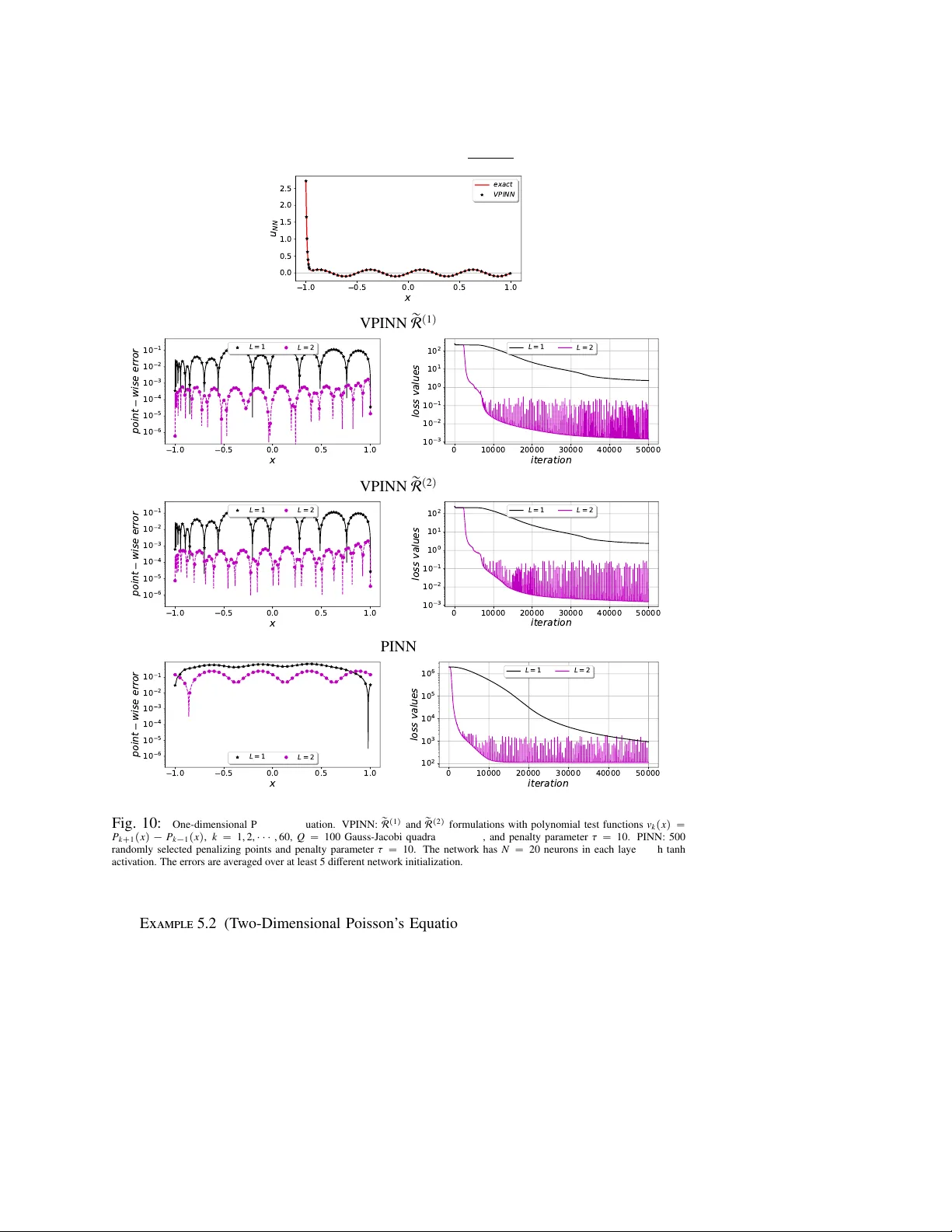
VPINNs: V ARIA TIONAL PHYSICS-INFORMED NEURAL NETWORKS FOR SOL VING P ARTIAL DIFFERENTIAL EQU A TIONS ˚ EHSAN KHARAZMI : , ZHONGQIANG ZHANG ; , GEORGE EM KARNIADAKIS §¶ Abstract. Physics-informed neural networks (PINNs) [ 31 ] use automatic di ff erentiation to solve partial di ff er- ential equations (PDEs) by penalizing the PDE in the loss function at a random set of points in the domain of interest. Here, we de velop a Petrov-Galerkin version of PINNs based on the nonlinear approximation of deep neural networks (DNNs) by selecting the trial space to be the space of neural netw orks and the test space to be the space of Legendre polynomials. W e formulate the variational residual of the PDE using the DNN approximation by incorporating the variational form of the problem into the loss function of the network and construct a variational physics-informed neural network (VPINN). By integrating by parts the inte grand in the variational form, we lo wer the order of the dif- ferential operators represented by the neural networks, hence e ff ecti vely reducing the training cost in VPINNs while increasing their accuracy compared to PINNs that essentially emplo y delta test functions. For shallo w networks with one hidden layer , we analytically obtain explicit forms of the variational r esidual . W e demonstrate the performance of the new formulation for several examples that show clear advantages of VPINNs over PINNs in terms of both accuracy and speed. Key word. physics-informed learning, PINNs, v ariational neural network, automatic di ff erentiation, PDE, Petrov-Galerkin formulation 1. Introduction. Dev eloping e ffi cient and accurate numerical methods for simulating the multiscale dynamics of physical and biomedical phenomena has been a long-standing challenge in scientific computing. Se veral methods ha ve been de veloped in the literature that aim to provide stable, con v ergent and accurate approximations of the partial di ff erential equa- tions (PDEs) that govern multiscale dynamics. The most popular and standard approaches are finite di ff erence, finite element and spectral methods. These methods generally con vert the mathematical model into its discrete counterpart using a grid o ver the computational do- main and then solve the resulting linear or nonlinear system of PDEs for the unkno wn state variables at the nodes of the grid or for the unknown coe ffi cients of functional expansions describing these state variables. Spectral methods, in particular , consider a linear combina- tion of some kno wn basis (trial) functions as a modal / nodal approximation, where the span of these basis functions constructs a conv ergent discrete solution space of the problem. The resulting system of unknown coe ffi cients is then obtained by testing the equation with suit- able test functions. In a Petrov-Galerkin setting, the trial basis and test function spaces are distinct and hence di ff erent choices yield di ff erent numerical schemes, while in the Galerkin framew ork the trial basis functions and test functions are identical. These methods have been significantly advanced ov er the past five decades and successfully employed in simulating physical and biological problems, e.g. [ 22 ] and the references therein. In a more general setting, a di ff erent technique put forward more recently is the nonlin- ear approximation [ 11 , 12 ], which extends the approximants to belong to a nonlinear space and does not limit the approximation to linear spaces, leading to a more robust estimation by sparser representation and cheaper computation. The nonlinear approximation contains di ff erent approaches including wa velet analysis [ 7 ], dictionary learning [ 35 ], adaptive pur- : Division of Applied Mathematics, Brown University , 170 Hope st., Providence , RI 02906, USA. Email: ehsan kharazmi@brown.edu ; Department of Mathematical Sciences, W orcester Polytechnic Institute, 100 Institute Rd, W orcester , MA 01609, USA. Email: zzhang7@wpi.edu § Division of Applied Mathematics, Brown University , 170 Hope st., Providence , RI 02906, USA. Email: george karniadakis@brown.edu ¶ Pacific Northwest National Laboratory , Richland, W A 99354, USA. ˚ This work was supported by the Applied Mathematics Program within the Department of Energy on the PhILMs project (DESC0019434 and DE-SC0019453). 1 2 suit and compressed sensing [ 9 , 27 , 4 , 5 ], adaptive splines [ 11 ], radial basis functions [ 10 ], Gaussian kernels [ 16 ], and neural networks [ 24 , 26 , 8 ]. F or example, for functions in Besov spaces with smoothness s and input dimensionality of d , it has been sho wn that an approxi- mation of order O p N ´ s { d q that is almost optimal can be constructed [ 10 , 16 , 23 ]. Moreover , for H ¨ older continuous functions of order 1 on r 0 , 1 s d , an O p´ 1 2 d q approximation was constructed in [ 38 ] and then further improved to O p´ 2 d q in [ 33 ]. While nonlinear approximation presents more capabilities, its nonlinear nature imposes extra complications, and achieving the optimal approximation rate, especially in high dimensional spaces, remains an ongoing challenging problem. A neural network (NN), and in particular a deep NN (DNN), can be built to construct a relation u N N p x q : Ω Ñ R between a high-dimensional input x P Ω Ă R d with some positiv e integer d and the output u N N P R via algebraic operations and nonlinear mapping. One of the main advantages of DNNs is that they can represent a large family of functions with a relati vely small number of parameters. It w as sho wn in [ 6 ] that a two-layer (containing only a single hidden layer) network has great expressi ve po wer , and in particular a two- layer network with sigmoid acti vations could approximate any continuous function. It was also shown in [ 1 ] that a one-to-one correspondence between the class of ReLU DNNs and piecewise linear (PWL) functions can be established, which shows that any PWL function can be representable by a ReLU DNN. DNNs are generally comprised of input, output, and hidden layer(s), where each layer may contain several neurons. Assuming a fully connected network, the connection between neurons forms a complete graph. In this case, each interior hidden layer recei ves the information from the pre vious layer and passes it to the next layer after applying a combination of scaling (by some weights), shifting (by some biases), and a nonlinear mapping. The final output of the network is then a nonlinearly-mapped weighted summation of input and hidden layers with certain biases, where the weights w and biases b are called the unknown parameters of the network. As DNNs use nonlinear compositional mappings, usually there is no closed form solution of the network parameters, and they are obtained via iterati ve algorithms, e.g. back propagation, that minimizes a properly defined objectiv e (loss) function. Generally , the loss function is designed as a discrepanc y measure between the network output u N N and the given data u , where its minimization returns the parameters that best approximate the solution. This process of loss minimization is called network training, and a trained network has usually “optimum” parameters that can accurately represent the training data sets, while its performance over any other admissible input data (test data) should be examined. In most of practical applications of NN, the constructed network can be thought of being ignorant of any possibly existing underlying mathematical model expressing physical laws, and therefore gi ves a model-ignorant algorithm as the network training process does not re- quire any knowledge of the underlying mathematical model. Recently , NNs ha ve been con- structed such that they incorporate the underlying mathematical model in the network graph and construct a physics-informed neural network (PINN) [ 31 ]. The loss function contains extra terms to merge the mathematical model as an additional constraint to ensure that the network output satisfies the mathematical model as well. F or accurate and reliable training, model-ignorant networks require a fairly large number of high fidelity training data points, which are in general expensi ve to obtain. The physics-informed approach, howev er , replaces such large volume data requirement by infusing information from the underlying physics by forcing the network output to satisfy the corresponding mathematical model at some penal- izing points that are av ailable at minimal cost, and thus the network only requires a minimal number of expensi ve training data. The recent de velopment of PINNs has been well estab- lished for forward and inv erse problem of solving di ff erential equations [ 30 , 32 , 39 , 29 ] and 3 since then a number of extensions has been made to tackle sev eral physical and biomedical problems [ 28 , 18 , 19 ]. All of these formulations employ the strong form of the mathemati- cal models into the network, i.e., the conservation laws are enforced at random points in the space-time domain. In this paper , we develop a v ariational physics-informed neural netw ork (VPINN) within the Petrov-Galerkin framework, where the solution is represented by nonlinear approximation via a (deep) neural network, while the test functions still belong to linear function spaces. Un- like a PINN that incorporates the strong form of the equation into the network, we incorporate the v ariational (weak) formulation of the problem and construct a variational loss function . The advantages of the v ariational formulation are multi-fold: ‚ The order of di ff erential operators can be e ff ectively reduced by proper integration- by-parts, which reduces the required re gularity in the (nonlinear) solution space. This will further mitigate the comple xity of PINNs in taking high-order deriv ativ es of nonlinear compositional functions, leading to less computationally expensiv e al- gorithms. ‚ In the case of shallow networks and for special activ ation and test functions, the loss function can be e xpressed analytically , which opens up the possibility of performing numerical analysis of such formulations. ‚ The lar ge number of penalizing points required by PINNs is replaced by a relati vely small number of quadrature points that are used to compute the corresponding inte- grals in the variational formulation. ‚ This setting can benefit from domain decomposition into man y sub-domains, where in each sub-domain we can use a separate number of test functions based on the local regularity of the solution. This yields a local (elemental) more fle xible learning approach. The rest of the paper is organized as follows. In section 2 , we briefly discuss the nonlinear function approximation of DNNs. In section 3 , we formulate the proposed VPINN, and then carry out the analytical approach in the deriv ation of variational residuals for shallow networks in section 4 . W e tak e the formulation to deeper networks in section 5 . Each section is supported by sev eral numerical examples to demonstrate the performance of the proposed method. W e conclude the paper with a summary section 6 . 2. Nonlinear Function Appr oximation. In general, a nonlinear approximation identi- fies the optimal approximant as a linear composition of some nonlinear approximators. Let x P Ω Ă R d and u : Ω Ñ R be a target function in a Hilbert space associated with some proper norm } ¨ } ‹ such as L 2 or L 8 norm. A DNN, comprised of L hidden layers with N i neurons in each layer and activ ation function σ , is a po werful nonlinear approximation that takes the compositional form u p x q « ˜ u p x q “ l ˝ T p L q ˝ T p L ´ 1 q ˝ ¨ ¨ ¨ ˝ T p 1 q p x q . (2.1) The nonlinear mapping in each hidden layer i “ 1 , 2 , ¨ ¨ ¨ , L is T p i q p¨q “ σ p W i ˆ ¨ ` b i q with weights W i P R N i ˆ N i ´ 1 and biases b i P R N i , where N 0 “ d is the input dimension. The output of the last hidden layer is finally mapped via the liner mapping l : R N L Ñ R to the network output. W e note that the acti vation function σ has similar form for each neuron, ho wever , it may also have di ff erent domain and image dimensionality based on the structure of network [ 20 , 19 ]. For a specific network structure (depth L and width N ) and a choice of activ ation func- tion, DNN ( 2.1 ) seeks an approximation that minimizes an objecti ve function that measures the discrepancy of NN output and the gi ven target function, i.e. } u p x q ´ ˜ u p x q} ‹ . Therefore, the approximated function is obtained as u ˚ p x q “ arg min W , b } u p x q ´ ˜ u p x q} ‹ . This minimization 4 problem, ho wev er, is not tri vial as usually DNNs take high dimensional inputs and hav e deep structures that can lead to some numerical issues such as local minima traps, and in practice, one finds ˆ u p x q « u ˚ p x q as the approximation. Hence, the accuracy of DNNs can be charac- terized by di viding the expected error into three main types: approximation error } ˜ u ´ u } ‹ , generalization error } u ˚ ´ ˜ u } ‹ , and optimization error } ˆ u ´ u ˚ } ‹ . There hav e been se veral works in the literature [ 21 , 8 , 25 , 34 , 14 , 33 ], which attempt to identify these di ff erent sources of error and de velop a proper framework for error analysis of deep NN. Achie ving an optimal approximation, howe ver , depends on man y factors and it still remains an open problem. 3. V ariational Physics-Inf ormed Neural Networks (VPINNs). In general, the under- lying gov erning equation of a physical problem in steady state can be written as L q u p x q “ f p x q , x P Ω (3.1) u p x q “ h p x q , x P B Ω (3.2) ov er the physical domain Ω Ă R d with dimensionality d and boundaries B Ω . The quantity u p x q : Ω Ñ R describes the underlying physics, the forcing f p x q is some (su ffi ciently) known external excitation, and L usually contains di ff erential and / or integro-di ff erential operators with parameters q . A proper numerical method obtains the approximate solution ˜ u p x q « u p x q to the abov e set of equations, while satisfying the boundary / initial conditions is a critical k ey in the stability and con ver gence of the method. ‚ PINNs : A solution of equations ( 3.1 ) and ( 3.2 ) can be obtained by employing a DNN as approximated solution, i.e. u p x q « ˜ u p x q “ u N N p x ; w , b q , where u N N is a neural network output with weights and biases t w , b u , respecti vely . This results in a physics-informed neural network (PINN), which was first introduced in [ 31 ]. The PINN algorithm infuses the gov- erning equation to the network by forcing the network output to satisfy the corresponding mathematical model in the interior domain and at boundaries. Let x r P Ω and x u P B Ω be some interior and boundary points, respectiv ely . W e define the str ong-form r esidual as re sidual s “ r p x q ´ r b p x q , (3.3) r p x q “ L q u N N p x q ´ f p x q , @ x P x r , r b p x q “ u N N p x q ´ h p x q , @ x P x u . Subsequently , we define the str ong-form loss function as L s “ L s r ` L u , (3.4) L s r “ 1 N r N r ÿ i “ 1 ˇ ˇ ˇ r p x r i q ˇ ˇ ˇ 2 , L u “ τ 1 N u N u ÿ i “ 1 ˇ ˇ ˇ r b p x u i q ˇ ˇ ˇ 2 , in which τ denotes a penalty parameter . Here, we use the superscript s to refer to the loss function associated with the strong form of residual and also later to distinguish between this from and other considered cases. In this setting, we pose the problem of solving ( 3.1 ) and ( 3.2 ) as: find ˜ u p x q “ u N N p x ; w ˚ , b ˚ q such that t w ˚ , b ˚ u “ argmin p L s p w , b qq . (3.5) The approximated solution u N N in PINNs does not necessarily satisfy the boundary con- ditions. Therefore, we see that the strong-form loss function is comprised of two parts: the first part that penalizes the strong-form residual at some interior (penalizing) points x r , and the 5 × × × × × × × × × × × × × × × × × × × × × × × × × × × × × × × × × × × × × × × × × Inte rior tra ini ng point s Boun dary tra ining points Inte rior pena li zi ng point s Fig. 1: A schematic of training and penalizing points on a complicated domain in evaluation of strong-form loss function L s p w , b q . The squares are training points scattered around on the domain boundary and triangles are a few interior training points. The crosses are penalizing points, which are largely av ailable in millions as mini batch sizes can be used. W e note that the training points can include some interior points as well, which can e ffi - ciently add the known information from the interior domain to the training algorithm; see [ 31 ] for more details. second part that penalizes the solution at boundary (training) points x u , leading to a penalty- like method. Fig. 1 schematically sho ws these points in an arbitrary domain. Several spectral penalty methods ha ve been de veloped in the literature, see e.g. [ 13 , 17 , 36 ]. In general, these penalty methods construct a unified equation by e ffi ciently adding the boundary conditions to the interior governing equation via a penalty term. This term includes a penalty function Q p x q and a penalty parameter τ that are designed such that the corresponding scheme maintains the coercivity in proper function spaces and norms. In the context of spectral methods, a penalty term is required when the basis functions do not naturally satisfy the boundary conditions, and in polynomial pseudospectral (or collocation) methods Q p x q takes similar polynomial form as the interpolation polynomials [ 13 ]. There is no analysis in the literature that formulates PINNs in the form of a penalty method. Thus, the penalty parameter τ in the strong-form loss function depends on the problem at hand and designed based on numerical e xperiments but it can also be set as a hyperparameter . ‚ VPINNs : Here, we develop the ne w setting of v ariational physics-informed neural netw ork, which is inspired by the variational form of the mathematical problem. W e let the approxi- mation form ˜ u p x q “ u N N p x ; w , b q with weights and biases t w , b u , respectively . W e also let v p x q be a properly chosen test function. W e multiply ( 3.1 ) by the test function and integrate ov er the whole domain to obtain the variational form p L q u N N p x q , v p x q q Ω “ p f p x q , v p x q q Ω (3.6) u p x q “ h p x q , x P B Ω (3.7) where p¨ , ¨q denotes the usual inner product. This variational form leads to the variational r esidual , defined as Re sid ual v “ R ´ F ´ r b , (3.8) R “ p L q u N N , v q Ω , F “ p f , v q Ω , which is enforced for any admissible test function v k , k “ 1 , 2 , ¨ ¨ ¨ and r b has the same form as in ( 3.3 ). Hence, we construct a discrete finite dimensional space V K by choosing a finite set of admissible test functions and let V K “ span t v k , k “ 1 , 2 , ¨ ¨ ¨ , K u . Subsequently , we define the variational loss function as L v “ L v R ` L u , (3.9) L v R “ 1 K K ÿ k “ 1 ˇ ˇ ˇ R k ´ F k ˇ ˇ ˇ 2 , L u “ τ 1 N u N u ÿ i “ 1 ˇ ˇ ˇ r b p x u i q ˇ ˇ ˇ 2 , in which τ denotes the penalty parameter . Here, we use the superscript v to refer to the loss function associated with the variational form of residual. In this setting, we pose the problem of solving ( 3.6 ) and ( 3.7 ) as: find ˜ u p x q “ u N N p x ; w ˚ , b ˚ q such that t w ˚ , b ˚ u “ argmin p L v p w , b qq . (3.10) 6                󰇛  󰇜     Input la y er Hidden la y er Output la y er V ari at iona l Form of Go verning Equation V ariation al Loss thresh ol d 󰇛     󰇜   󰇛    󰇜                                            T est Functi ons           󰇻      󰇛     󰇜   󰇛    󰇜                               Fig. 2: Schematic of VPINN in a Petrov-Galerkin formulation. Trial functions belong to the space of NN and test functions can be chosen from a separate NN or other function spaces such as polynomials and trigonometric functions. Red color represents the di ff erential operators on trial space. Green color represents the test functions and their deriv atives. Blue color represents the variational residuals R . R emark 3.1 (Analogy between strong-form and variational residual). A similar analogy as in standard numerical schemes to solve the strong and variational (weak) forms of di ff er- ential equations can be constructed her e too. Loosely speaking, by adopting the delta dirac function as the test function, i.e. v k p x q “ δ p x ´ x k q , the variational residual ( 3.8 ) becomes the str ong-form r esidual, given in ( 3.3 ) evaluated at (penalizing point) x k : R k ´ F k “ p L q u N N p x q , v k p x q q Ω ´ p f p x q , v k p x q q Ω “ p L q u N N p x q , δ p x ´ x k q q Ω ´ p f p x q , δ p x ´ x k q q Ω “ L q u N N p x k q ´ f p x k q “ r p x k q . Ther efor e, in the str ong-form, we evaluate the residual at some penalizing points while there ar e no such points in the variational form and instead we test the r esidual with a set of test functions. A major challenge in VPINN, unlike PINN, is to compute the integrals in the loss func- tion. The compositional structure of neural networks makes it almost impossible to obtain analytic expression of these integrals. Their computation is also not fully practically feasible as ev en in the case of network with two hidden layer there is no analysis for their quadrature rules. In order to av oid such a complication, we first choose a shallow network with one hidden layer . This enables us to carry out the deri vations analytically at least for some special cases. Then, we will introduce deep VPINNs by composing se veral hidden layers and consid- ering deep networks, where we need to employ numerical integration techniques to compute the integrals in the v ariational residuals. 4. Shallow VPINNs. W e consider a shallow neural network with one hidden layer and N neurons. W e let u p x q : Ω Ñ R , where Ω “ p´ 1 , 1 q , and consider the following boundary value problem ´ d 2 u p x q d x 2 “ f p x q , x P p´ 1 , 1 q (4.1) u p´ 1 q “ g , (4.2) 7 u p 1 q “ h , where h and g are constants and we assume the force term f p x q is fully av ailable (this assump- tion can be relaxed as we do not need the force term to be av ailable at all points). Let the approximate solution be u p x q « ˜ u p x q “ u N N p x q , then the strong-form residual ( 3.3 ) becomes re sidual s “ r p x q ´ r b p x q (4.3) r p x q “ ´ d 2 u N N p x q d x 2 ´ f p x q , x P p´ 1 , 1 q , r b p x q “ u N N p x q ´ u p x q , x “ ˘ 1 . W e choose a set of test functions v k p x q P V K with compact support on Ω such that v k p x q “ # non-zero , x P p´ 1 , 1 q , 0 , else where , k “ 1 , 2 , ¨ ¨ ¨ , K . (4.4) The variational residual ( 3.8 ) then becomes Re sid ual v k “ R k ´ F k ´ r b (4.5) R k “ ´ ˆ d 2 u N N p x q d x 2 , v k p x q ˙ Ω , F k “ p f p x q , v k p x q q Ω , where r b is giv en in ( 4.3 ). By integrating by parts in the first term R k , we can define three distinctiv e variational r esidual forms, namely R p 1 q k “ ´ ˆ d 2 u N N p x q d x 2 , v k p x q ˙ Ω , (4.6) R p 2 q k “ ˆ d u N N p x q d x , d v k p x q d x ˙ Ω ´ d u N N p x q d x v k p x q ˇ ˇ ˇ ˇ B Ω , (4.7) R p 3 q k “ ´ ˆ u N N p x q , d 2 v k p x q d x 2 ˙ Ω ´ d u N N p x q d x v k p x q ˇ ˇ ˇ ˇ B Ω ` u N N p x q d v k p x q d x ˇ ˇ ˇ ˇ B Ω . (4.8) The corresponding variational loss function s for each case take the form L v p i q “ L v p i q R ` L u , i “ 1 , 2 , 3 , (4.9) L v p i q R “ 1 K K ÿ k “ 1 ˇ ˇ ˇ R p i q k ´ F k ˇ ˇ ˇ 2 , L u “ τ 2 ˆ ˇ ˇ ˇ u N N p´ 1 q ´ g ˇ ˇ ˇ 2 ` ˇ ˇ ˇ u N N p 1 q ´ h ˇ ˇ ˇ 2 ˙ , R emark 4.1. Because the test functions have compact support o ver Ω , the first boundary term in ( 4.7 ) and ( 4.8 ) vanishes. Mor eover , by c hoosing a pr oper weight coe ffi cient τ in ( 4.9 ) , we make sur e that the network learns the boundary accurately . Therefor e, we replace the second boundary term in ( 4.8 ) by the exact values at boundaries. Hence, we have d u N N p x q d x v k p x q ˇ ˇ ˇ ˇ B Ω “ 0 , u N N p x q d v k p x q d x ˇ ˇ ˇ ˇ B Ω « u p x q d v k p x q d x ˇ ˇ ˇ ˇ B Ω . 4.1. Shallow VPINN With Sine Activation Functions And Sine T est Functions. A shallow network with one hidden layer has a relatively simple representation, which enables us to carry out the integrals analytically . Denoting the weights and biases associated with the 8 Fig. 3: A shallow neural network with one hidden layer , N neurons, and activ ation func- tion σ . W e let u N N j p x q “ a j σ p w j x ` θ j q and u N N p x q “ ř N j “ 1 u N N j p x q . 𝑥 𝜎 𝜎 𝑢 𝜎 𝑤 1 𝜃 1 𝑎 1 𝑤 𝑗 𝜃 𝑗 𝑎 𝑗 𝑤 𝑁 𝜃 𝑁 𝑎 𝑁 first layer by w j and θ j , respectiv ely , and the weights associated with the output by a j , we construct the neural network with N neurons and represent the approximate solution as u N N p x q “ N ÿ j “ 1 u N N j p x q “ N ÿ j “ 1 a j sin p w j x ` θ j q , (4.10) where σ “ sin is the activ ation function. Figure 3 sho ws the schematic of the network. W e also choose the test functions to be sine functions of the form v k p x q “ sin p k π x q , k “ 1 , 2 , ¨ ¨ ¨ , K . (4.11) The deriv ation of variational residuals is not complicated but requires careful use of se veral trigonometric identities. W e present the full deri vations in the Appendix A and only present the final results here. The variational residuals ( 4.6 )-( 4.8 ) become R p 1 q k “ R p 2 q k “ 2 p´ 1 q k k π N ÿ j “ 1 a j w 2 j cos p θ j q sin p w j q w 2 j ´ k 2 π 2 , (4.12) R p 3 q k “ 2 p´ 1 q k k π N ÿ j “ 1 a j k 2 π 2 cos p θ j q sin p w j q w 2 j ´ k 2 π 2 ` p´ 1 q k k π p h ´ g q . (4.13) W e note that the variational forms ( 4.6 ) and ( 4.7 ) hav e exact similar analytical expression, howe ver , the form ( 4.8 ) is di ff erent due to the additional boundary approximation explained in Remark 4.1 . ‚ Steady Burger’ s Equation: The Burger’ s equation is one of the fundamental PDEs arising in various physical fields, including nonlinear acoustics, gas dynamics, and fluid mechanics; see e.g. [ 37 ] and references therein. This equation was first introduced in [ 2 ] and then later in the conte xt of theory of turb ulence was studied in [ 3 ]. Here, we study the one-dimensional steady state Burger’ s equation, given as u d u d x ´ d 2 u d x 2 “ f p x q , (4.14) u p´ 1 q “ g , u p 1 q “ h . The variational residual ( 3.8 ) for this problem becomes Re sid ual v k “ R k ` R N L k ´ F k ´ r b , (4.15) in which R N L k “ ˆ u N N p x q d u N N p x q d x , v k p x q ˙ Ω , (4.16) 9 and other terms are the same as in ( 4.5 ). The corresponding variational loss function s for this problem can be written as L v p i q “ L v p i q R ` L u , L v p i q R “ 1 K K ÿ k “ 1 ˇ ˇ ˇ R p i q k ` R N L k ´ F k ˇ ˇ ˇ 2 , i “ 1 , 2 , 3 . (4.17) The shallow netw ork ( 4.10 ) with test functions ( 4.11 ) gives R N L k “ p´ 1 q k k π N ÿ i “ 1 N ÿ j “ 1 a i a j w i „ sin p w j ` w i q cos p θ j ` θ i q p w j ` w i q 2 ´ k 2 π 2 ` sin p w j ´ w i q cos p θ j ´ θ i q p w j ´ w i q 2 ´ k 2 π 2  . (4.18) The detailed deriv ation is gi ven in the appendix. ‚ Numerical Examples: Here, we examine the performance of our proposed method using a shallo w network with sine activ ation function to solve the steady state Burger’ s equation. W e also employ sine test functions and train the network using the loss function defined in ( 4.17 ). E xample 4.2. W e consider equation ( 4.14 ) and let the e xact solution, boundary values, and for ce term be of the form u e xact “ A sin p ω x q , g “ A sin p´ ω q , h “ A sin p ω q , f p x q “ A 2 ω { 2 sin p 2 ω x q ` A ω 2 sin p ω x q . W e show the r esults for variational forms R p 1 q and R p 2 q in F igs. 4 - 5 , and for variational form R p 3 q in F ig. 6 . T able 1: One dimensional steady state Burger’ s equation: Neural network, optimizer, and VPINN parameters. VPINN variational form R p 1 q , R p 2 q , R p 3 q # test functions 5 test functions sin p k π x q τ 5 NN # hidden layers 1 # neurons in each hidden layer 5 activ ation function sine optimizer Adam learning rate 10 ´ 3 1.0 0.5 0.0 0.5 1.0 x 1.0 0.5 0.0 0.5 1.0 u N N e x a c t V P I N N 1.0 0.5 0.0 0.5 1.0 x 0 1 2 3 4 5 6 p o i n t w i s e e r r o r 1e 7 Fig. 4: One-dimensional steady state Burger’ s equation: VPINN with R p 1 q “ R p 2 q formulation. Left: exact solution sin p 2 . 1 π x q and VPINN approximation. Right: point-wise error av eraged over several random network initializations. See T able 1 for VPINN hyperparameters. 10 0 5000 10000 15000 20000 i t e r a t i o n 1 0 1 4 1 0 1 0 1 0 6 1 0 2 1 0 2 l o s s v a l u e s r a n d o m i n i t i a l i z a t i o n # 1 r a n d o m i n i t i a l i z a t i o n # 2 1.0 0.5 0.0 0.5 1.0 x 0.0 0.2 0.4 0.6 0.8 p o i n t w i s e e r r o r 1e 6 L n o r m : O ( 1 0 9 ) L n o r m : O ( 1 0 6 ) Fig. 5: One-dimensional steady state Burger’ s equation: network initialization e ff ect on optimization performance. Left: com- parison of loss values. Right: comparison of point-wise error . The red dashed line shows a more successful optimization and thus a much lower error . See T able 1 for VPINN hyperparameters. 1.0 0.5 0.0 0.5 1.0 x 0 1 2 3 4 p o i n t w i s e e r r o r 1e 4 = 1 = 2 = 5 = 1 0 = 1 5 0 10000 20000 30000 40000 50000 i t e r a t i o n 1 0 5 1 0 3 1 0 1 1 0 1 1 0 3 l o s s v a l u e s = 1 = 2 = 5 = 1 0 = 1 5 1.00 0.95 0.90 0.85 0.80 x 0 1 2 3 4 p o i n t w i s e e r r o r 1e 4 0.80 0.85 0.90 0.95 1.00 x 0 1 2 3 4 p o i n t w i s e e r r o r 1e 4 Fig. 6: One-dimensional steady state Burger’ s equation: e ff ect of penalty parameter τ in the R p 3 q formulation. T op Left: comparison of exact solution sin p 2 . 1 π x q and VPINN approximation for di ff erent τ . T op Right: loss value. Bottom: the zoom-in display of point-wise error close to boundaries. See T able 1 for VPINN hyperparameters. ‚ Discussion: In Example 4.2 , the e xact solution is the sine function with a fixed frequency ω . In the de veloped VPINN to solve this problem, we construct a shallow network of one hidden layer with N neurons and sine activ ation function. Therefore, each neuron represents a sine function with adaptiv e frequency w j . Ideally , one neuron would be su ffi cient to ex- actly capture the solution if the neuron frequency w j could be precisely optimized to exact frequency ω . This is not the case in practice howe ver , as the optimizer may fail to con v erge if the netw ork initialization is very far from the target v alues. In general, weights and biases are initialized from known probability distributions. Xavier initialization [ 15 ] is one of the most widely used initialization method, which initializes the weights in the network by drawing them from a distribution with zero mean and a finite variance. The optimal value of v ariance is given 1 { N , where N is the number of nodes feeding into that layer . This optimal value, howe ver , leads to optimizer failure in our VPINN formulation for the problem at hand. This is due to the fact that the neuron frequencies are initially drawn from a very narrow distribu- tion and therefore they may fall very far from the target frequency . T o a void this failure, we need to widen the distribution and increase the number of neurons to make sure at least one of the neuron frequencies will fall close enough to the target frequency . W e also note that the construction of force vector is carried out exactly and we do not use an y quadrature rules. Therefore, we can isolate the error associated with the optimization process of the network. 11 Figure 4 shows the point-wise error , averaged over sev eral di ff erent random network initial- izations. In the most successful case of optimization, we report the L 8 -norm error of order 10 ´ 9 for this specific problem. In the formulation of R p 3 q in ( 4.8 ) and then later in ( 4.13 ) for a shallow network, we use Remark 4.1 to replace the boundary terms in the variational loss with the exact kno wn boundary conditions. In this case, the con ver gence of error depends strongly on how well the network learns the boundary conditions, in that any error from the inaccurate approximation of the boundary condition will propagate through the interior domain. Therefore, by increas- ing the penalty coe ffi cient in the loss function, we mitigate the error at the boundaries and contain its adverse propagation to the interior domain; see Fig. 6 . The PINN formulation with sine activ ation function fails to lead to an accurate approx- imation. W e used a shallow network with single hidden layer, N “ 50 neurons, N r “ 1000 penalizing points, and obtained the L 8 approximation error of or O p 1 q . W e note, howe ver , that the choice of tanh activ ation function performs much more accurately , and with similar network structure results in L 8 approximation error of or O p 10 ´ 5 q . This is still not compara- ble with VPINN, as in VPINN, we obtain a much more accurate result with a much simpler network. E xample 4.3. W e consider equation ( 4.14 ) , however , we let the exact solution vanish at the two boundaries, i.e. u e xact “ A p 1 ´ x 2 q sin p ω x q , g “ h “ 0 . The for ce term f p x q can be obtained easily by substituting u e xact in ( 4.14 ) . W e show the err or con ver gence by incr easing the number of neur ons and test functions for variational forms R p 1 q “ R p 2 q and R p 3 q in F ig. 7 . In all cases, the value of the penalty parameter is fixed to τ “ 100 . ‚ Discussion: W e first consider the projection of the exact solution u e xact onto the network. By using the sine test functions ( 4.11 ), we introduce the v ariational residual of projection and the loss function as u e xact « u N N p x q “ N ÿ j “ 1 a j sin p w j x ` θ j q , R pro j k “ p u N N p x q , v k p x q q Ω , U k “ p u e xact p x q , v k p x q q Ω , L pro j “ 1 K K ÿ k “ 1 ˇ ˇ ˇ R p k ´ U k ˇ ˇ ˇ 2 ` τ ˆ ˇ ˇ ˇ u N N p´ 1 q ´ g ˇ ˇ ˇ 2 ` ˇ ˇ ˇ u N N p 1 q ´ h ˇ ˇ ˇ 2 ˙ . Follo wing similar steps as in ( 4.13 ), we can obtain an analytical expression of the v ariational residual, R pro j k “ 2 p´ 1 q k k π N ÿ j “ 1 a j cos p θ j q sin p w j q w 2 j ´ k 2 π 2 . (4.19) The con vergence of u N N p x q Ñ u e xact by minimizing the loss function L pro j depends strongly on the number of neurons N , number of test functions K , and performance of optimization. W e observe that we can obtain the best L 8 projection error of order O p 10 ´ 4 q by choosing N “ K “ 5, where any other combination leads to less accurate results. In solving the di ff erential equation, we expect VPINN to giv e an accuracy level of almost similar order as the projection. In example 4.3 , the periodic boundary conditions simplifies the R p 3 q formulation 12 u e xact “ p 1 ´ x 2 q sin p 2 . 1 π x q 1.0 0.5 0.0 0.5 1.0 x 1.0 0.5 0.0 0.5 1.0 u N N e x a c t V P I N N R p 2 q Formulation 1.0 0.5 0.0 0.5 1.0 x 0.0 0.2 0.4 0.6 0.8 1.0 p o i n t w i s e e r r o r 1e 4 N = K = 4 N = K = 5 N = K = 6 0 10000 20000 30000 40000 50000 i t e r a t i o n 1 0 1 4 1 0 1 0 1 0 6 1 0 2 1 0 2 l o s s v a l u e s N = K = 4 N = K = 5 N = K = 6 R p 3 q Formulation 1.0 0.5 0.0 0.5 1.0 x 0.0 0.2 0.4 0.6 0.8 1.0 p o i n t w i s e e r r o r 1e 4 N = K = 4 N = K = 5 N = K = 6 0 10000 20000 30000 40000 50000 i t e r a t i o n 1 0 1 4 1 0 1 0 1 0 6 1 0 2 1 0 2 l o s s v a l u e s N = K = 4 N = K = 5 N = K = 6 Fig. 7: Example 4.3 . One-dimensional steady state Burger’ s equation: error conver gence by increasing N (number of neurons) and K (number of test functions). Shallow network with L “ 1 hidden layer, sine acti vation, and sine test function. by removing the term p h ´ g q in ( 4.13 ). Howe ver , the approximation in Remark 4.1 still exists, and thus, R p 3 q does not necessarily perform better , compared to the other formulations. W e see that by increasing the number of neurons and test functions, the error over the whole domain decreases. It will, ho wever , saturate at some points, where the optimization error becomes dominant. In general, we can decompose the expected error associated with VPINN into four main types: NN approximation (expressi vity of NN), spectral projection, numerical integration, and optimization. Y et, it is hard to isolate single sources in the analysis of error as they are strongly related to each other . High expressivity , i.e. higher number of neurons N in the network, may complicate the loss function, leading to poor optimization performance. More importantly , the choice of sine acti vation function further requires additional care in network initialization, as was explained in example 4.2 . In our deriv ations for the shallow network, we remove the error of numerical integration by analytically expressing the loss functions. Then, by increasing N and K , we seek the best combination that leads to better accuracy . 4.2. Shallow Network with Sine Activation Functions and Polynomial T est Func- tions. By considering sine activ ation function, we construct a similar shallow network as in ( 4.10 ); also sho wn in Fig. 3 . Here, we choose a combination of Legendre polynomials as test 13 functions, i.e., v k p x q “ P k ` 1 p x q ´ P k ´ 1 p x q , k “ 1 , 2 , ¨ ¨ ¨ , K , (4.20) which naturally vanish at the boundary points v k p´ 1 q “ v k p 1 q “ 0. W e note that the construc- tion of variational residuals in this case is not unique, as one can use di ff erent properties of Jacobi polynomials to take the integrals and deriv e various formulations. W e use the recursion formula of Legendre polynomials to obtain the v ariational residuals ( 4.6 )-( 4.7 ). Therefore, R p 1 q k “ N ÿ j “ 1 a j w 2 j ż 1 ´ 1 sin p w j x ` θ j q p P k ` 1 p x q ´ P k ´ 1 p x q q d x (4.21) “ N ÿ j “ 1 a j w 2 j ż 1 ´ 1 Im t e i p w j x ` θ j q u p P k ` 1 p x q ´ P k ´ 1 p x q q d x “ N ÿ j “ 1 a j w 2 j Im e i θ j p I k ` 1 p w j q ´ I k ´ 1 p w j q q ( “ N ÿ j “ 1 a j w 2 j p C k ` 1 p w j q ´ C k ´ 1 p w j q q and R p 2 q k “ N ÿ j “ 1 a j w j ż 1 ´ 1 cos p w j x ` θ j q d d x p P k ` 1 p x q ´ P k ´ 1 p x q q d x (4.22) “ N ÿ j “ 1 a j w j ż 1 ´ 1 Re t e i p w j x ` θ j q u p 2 k ` 1 q P k p x q d x “ p 2 k ` 1 q N ÿ j “ 1 a j w j Re e i θ j I k p w j q ( “ p 2 k ` 1 q N ÿ j “ 1 a j w j B k ` 1 p w j q , where i “ ? ´ 1, Re t¨u and Im t¨u are the real and imaginary parts, respecti vely , and the following quantities I k p w j q “ ż 1 ´ 1 e iw j x P k p x q d x , C k p θ j , w j q “ Im e i θ j I k p w j q ( , B k p θ j , w j q “ Re e i θ j I k p w j q ( , hav e the following recursion formulas for k “ 2 , 3 , ¨ ¨ ¨ , K I k “ i 2 k ´ 1 w j I k ´ 1 ` I k ´ 2 , I 0 “ 2 sin p w j q w j , I 1 “ ´ 2 i w j ˆ sin p w j q ´ cos p w j q w j ˙ , C k “ 2 k ´ 1 w j B k ´ 1 ` C k ´ 2 , B 0 “ 2 sin p w j q cos p θ j q w j C 1 “ ´ 2 cos p θ j q w j ˆ sin p w j q ´ cos p w j q w j ˙ , B k “ ´ 2 k ´ 1 w j C k ´ 1 ` B k ´ 2 , C 0 “ 2 sin p w j q sin p θ j q w j , B 1 “ 2 sin p θ j q w j ˆ sin p w j q ´ cos p w j q w j ˙ . The full deriv ations of recursi ve formulas are giv en in Appendix B . ‚ Numerical Examples: Here, we consider the Poisson’ s equation as the analytical expres- sion of nonlinearity becomes very complicated, if not impossible, using polynomial test func- tions. Thus, ´ d 2 u d x 2 “ f p x q , u p´ 1 q “ g , u p 1 q “ h . (4.23) 14 The variational residual of the netw ork then becomes Re sid ual v k “ R k ´ F k ´ R b k , (4.24) and therefore, the corresponding variational loss function for this problem can be written as L v p i q “ 1 K K ÿ k “ 1 ˇ ˇ ˇ R p i q k ´ F k ˇ ˇ ˇ 2 ` τ 2 ˆ ˇ ˇ ˇ u N N p´ 1 q ´ g ˇ ˇ ˇ 2 ` ˇ ˇ ˇ u N N p 1 q ´ h ˇ ˇ ˇ 2 ˙ , i “ 1 , 2 . (4.25) E xample 4.4. W e consider equation ( 4.23 ) and let the exact solution be of the form u e xact “ A sin p ω x q ` tanh p r x q . The for ce term is simply obtained by substituting e xact solution in the equation. W e show the r esults for A “ 0 . 1 , ω “ 4 π , and r “ 5 in F ig. 8 . W e set the penalty parameter τ “ 10 . u e xact “ 0 . 1 sin p 4 π x q ` tanh p 5 x q 1.0 0.5 0.0 0.5 1.0 x 1.0 0.5 0.0 0.5 1.0 u N N e x a c t V P I N N 1.0 0.5 0.0 0.5 1.0 x 1 0 8 1 0 6 1 0 4 1 0 2 1 0 0 p o i n t w i s e e r r o r N = K = 2 N = K = 6 N = K = 1 0 N = K = 1 4 N = K = 1 8 0 10000 20000 30000 40000 50000 i t e r a t i o n 1 0 1 5 1 0 1 1 1 0 7 1 0 3 1 0 1 l o s s v a l u e s N = K = 2 N = K = 6 N = K = 1 0 N = K = 1 4 N = K = 1 8 Fig. 8: One-dimensional Poisson’s equation: error conv ergence by increasing number of neurons N and number of test functions K . VPINN: R p 1 q formulations of shallow network with L “ 1 hidden layer, sine activ ation, and Legendre test function. A shallow PINN with L “ 1 hidden layer, N “ 50 neurons, sine activ ation, and N r “ 1000 penalizing points has the L 8 error of O p 10 ´ 1 q . ‚ Discussion: The performance of VPINN by employing polynomial test functions ( 4.20 ) is much better compared to sine test functions ( 4.11 ) when the exact solution is not of a simple sinusoidal form. Howe ver , the analytical expression for the variational residual and the loss function become more complicated. When a high number of test functions is used, the recursion formulas lead to a high exponent of weights in the denominator , which makes the loss function very sensitiv e to the initialization of weights and biases. In Fig. 8 , we show the error conv ergence of a shallow VPINN for di ff erent number of neurons and test functions, based on variational residual R p 1 q ; we observe similar results for the formulation R p 2 q too. W e note that in Fig. 8 , the best approximation for N “ K “ 18 (blue line) has the highest loss value, compared to other cases. This shows that although the network has higher e xpressivity , the optimizer has more di ffi culty to train the network, and in case that the optimizer performs better , one can expect more accurate approximation by increasing N and K . Compared to a shallow PINN with L “ 1 hidden layer and sine activ ation, but a much 15 higher number of neurons, N “ 50, the network fails to accurately capture the exact solution and with N r “ 1000 penalizing points gives the L 8 error of O p 10 ´ 1 q . W e should mention that we choose the sine activ ation in PINN to compare with VPINN, howe ver , the tanh activ ation function can provide more accurate approximation in PINN; we further discuss this in the next section. 5. Shallow to Deep VPINNs. The advantage of neural networks is their high expres- sivity in their deep constructions. The composition of layers provides a high nonlinear repre- sentation of networks to more accurately approximate a function. On the other hand, unlike the shallo w networks, the analysis of deep constructions becomes more challenging as they do not lend themselves to simple analytical expressions. In the formulation of our proposed VPINN using deep neural networks, we cannot take the integrals of variational residuals an- alytically anymore and hav e to employ a numerical integration technique such as quadrature rules. Y et, there exist no works in the literature on analysis of quadrature integration for compositional function spaces of (deep) neural networks. In this section, we e xtend our for- mulation of shallo w VPINN to deep networks by employing Gauss type quadrature rules to compute the corresponding integrals in the loss function. Therefore, by choosing quadrature points and weights t x q , W q u q “ Q q “ 1 , test functions defined in ( 4.4 ) and by using Remark 4.1 , the variational residuals ( 4.6 )-( 4.8 ) can be written as R p 1 q k « r R p 1 q k “ ´ Q ÿ q “ 1 W q d 2 u N N p x q q d x 2 v k p x q q R p 2 q k « r R p 2 q k “ Q ÿ q “ 1 W q d u N N p x q q d x d v k p x q q d x R p 3 q k « r R p 3 q k “ ´ Q ÿ q “ 1 W q u N N p x q q d 2 v k p x q q d x 2 ` u p x q d v k p x q d x ˇ ˇ ˇ ˇ 1 ´ 1 which only requires the ev aluation of network (and / or its deriv ativ es) at sev eral quadrature points x q ’ s. The above approximation giv es us the flexibility to combine di ff erent choices of activ ation functions, test functions, and quadrature rules. 5.1. Numerical Examples. W e examine the performance of de veloped VPINN by con- sidering sev eral numerical examples with di ff erent exact solutions. In each case, we use the method of fabricated solutions and obtain the forcing term by substituting the exact solution into the corresponding equation. E xample 5.1 (One-Dimensional Poisson’ s Equation). W e consider the P oisson’s equa- tion given in ( 4.23 ) . W e let the exact solution be of di ff er ent forms steep solution: u e xact p x q “ 0 . 1 sin p 4 π x q ` tanh p 5 x q (5.1) boundary layer solution: u e xact p x q “ 0 . 1 sin p 4 π x q ` e 0 . 01 ´p x ` 1 q 0 . 01 (5.2) The force term is obtained by substituting u e xact p x q into the equation. W e show the results in F igs. 9 and 10 . ‚ Discussion: As expected, by increasing the number of hidden layer while keeping the other hyperparameters unchanged, we observe that the error drops by magnitudes of orders. This explicitly sho ws the expressi vity of deep networks compared to shallow ones. By employing similar optimizer , ho wev er, we see that the training process and loss conv ergence become less stable as there are large numbers of spikes in the loss value over the training iterations. W e 16 u e xact “ 0 . 1 sin p 4 π x q ` tanh p 5 x q 1.0 0.5 0.0 0.5 1.0 x 1.0 0.5 0.0 0.5 1.0 u N N e x a c t V P I N N VPINN r R p 1 q 1.0 0.5 0.0 0.5 1.0 x 1 0 8 1 0 7 1 0 6 1 0 5 1 0 4 1 0 3 p o i n t w i s e e r r o r L = 1 L = 2 0 10000 20000 30000 40000 50000 i t e r a t i o n 1 0 4 1 0 2 1 0 0 l o s s v a l u e s L = 1 L = 2 VPINN r R p 2 q 1.0 0.5 0.0 0.5 1.0 x 1 0 8 1 0 7 1 0 6 1 0 5 1 0 4 1 0 3 p o i n t w i s e e r r o r L = 1 L = 2 0 10000 20000 30000 40000 50000 i t e r a t i o n 1 0 4 1 0 2 1 0 0 l o s s v a l u e s L = 1 L = 2 PINN 1.0 0.5 0.0 0.5 1.0 x 1 0 8 1 0 7 1 0 6 1 0 5 1 0 4 1 0 3 p o i n t w i s e e r r o r L = 1 L = 2 0 10000 20000 30000 40000 50000 i t e r a t i o n 1 0 3 1 0 1 1 0 1 l o s s v a l u e s L = 1 L = 2 Fig. 9: One-dimensional Poisson’ s equation. VPINN: r R p 1 q and r R p 2 q formulations with polynomial test functions v k p x q “ P k ` 1 p x q ´ P k ´ 1 p x q , k “ 1 , 2 , ¨ ¨ ¨ , 60, Q “ 100 Gauss-Jacobi quadrature points, and penalty parameter τ “ 25. PINN: 500 randomly selected penalizing points and penalty parameter τ “ 10. The network has N “ 20 neurons in each layer with tanh activ ation. The errors are av eraged over at least 5 di ff erent network initializations. also observe that the depth of network changes the learning pattern as the sudden drop in the loss v alue plots happens much earlier . Compared to PINN, the results are relativ ely similar for the case of steep solution. Howe ver , for the boundary layer solution, VPINN performs much more accurately . In this case, for PINN to capture the very sharp boundary layer, we need to cluster a large number of penalizing points in the neighborhood of boundary layer . W e also note the oscillatory behavior of point-wise error in VPINN compared to PINN, which is expected due to the projection of neural network residuals onto the hierarchical polynomial test functions. 17 u e xact “ 0 . 1 sin p 4 π x q ` e 0 . 01 ´p x ` 1 q 0 . 01 1.0 0.5 0.0 0.5 1.0 x 0.0 0.5 1.0 1.5 2.0 2.5 u N N e x a c t V P I N N VPINN r R p 1 q 1.0 0.5 0.0 0.5 1.0 x 1 0 6 1 0 5 1 0 4 1 0 3 1 0 2 1 0 1 p o i n t w i s e e r r o r L = 1 L = 2 0 10000 20000 30000 40000 50000 i t e r a t i o n 1 0 3 1 0 2 1 0 1 1 0 0 1 0 1 1 0 2 l o s s v a l u e s L = 1 L = 2 VPINN r R p 2 q 1.0 0.5 0.0 0.5 1.0 x 1 0 6 1 0 5 1 0 4 1 0 3 1 0 2 1 0 1 p o i n t w i s e e r r o r L = 1 L = 2 0 10000 20000 30000 40000 50000 i t e r a t i o n 1 0 3 1 0 2 1 0 1 1 0 0 1 0 1 1 0 2 l o s s v a l u e s L = 1 L = 2 PINN 1.0 0.5 0.0 0.5 1.0 x 1 0 6 1 0 5 1 0 4 1 0 3 1 0 2 1 0 1 p o i n t w i s e e r r o r L = 1 L = 2 0 10000 20000 30000 40000 50000 i t e r a t i o n 1 0 2 1 0 3 1 0 4 1 0 5 1 0 6 l o s s v a l u e s L = 1 L = 2 Fig. 10: One-dimensional Poisson’ s equation. VPINN: r R p 1 q and r R p 2 q formulations with polynomial test functions v k p x q “ P k ` 1 p x q ´ P k ´ 1 p x q , k “ 1 , 2 , ¨ ¨ ¨ , 60, Q “ 100 Gauss-Jacobi quadrature points, and penalty parameter τ “ 10. PINN: 500 randomly selected penalizing points and penalty parameter τ “ 10. The network has N “ 20 neurons in each layer with tanh activ ation. The errors are av eraged over at least 5 di ff erent network initialization. E xample 5.2 (T wo-Dimensional Poisson’ s Equation). W e consider the following two- dimensional P oisson’s equation ∆ u p x , y q “ f p x , y q , (5.3) subject to homogeneous Dirichlet boundary conditions over Ω “ r´ 1 , 1 s ˆ r´ 1 , 1 s , wher e we assume that the forcing term f p x , y q is available at some quadratur e points. W e consider the exact solution as u e xact p x , y q “ p 0 . 1 sin p 2 π x q ` tanh p 10 x q q ˆ sin p 2 π y q , (5.4) 18 wher e the for cing function is obtained by substituting the e xact solution in ( 5.3 ) . W e show the r esults in F igs. 11 and 12 . T able 2: T wo-Dimensional Poisson’ s Equation: Neural network, optimizer , and VPINN parameters. VPINN variational form R p 2 q # test function K x “ 10 , K y “ 10 test functions P k ` 1 p . q ´ P k ´ 1 p . q # quadrature points Q x “ 70 , Q y “ 70 (Gauss-Lobatto) # (boundary) training points x : 2 ˆ 80, y : 2 ˆ 80 NN # hidden layers 4 # neurons in each layer 20 activ ation function sine optimizer Adam learning rate 10 ´ 3 Fig. 11: T w o-dimensional Poisson’ s equation. Left: exact solution ( 5.4 ). Middle: VPINN. Right: point-wise error. Neural network, optimizer , and VPINN parameters are given in T able 2 . x slices, — Exact, ‚ ‚ ‚ VPINN 1.0 0.5 0.0 0.5 1.0 x = 1 . 0 1.0 0.5 0.0 0.5 1.0 x = 0 . 6 1.0 0.5 0.0 0.5 1.0 x = 0 . 2 1.0 0.5 0.0 0.5 1.0 x = 0 . 2 1.0 0.5 0.0 0.5 1.0 x = 0 . 6 1.0 0.5 0.0 0.5 1.0 x = 1 . 0 y slices, — Exact, ‚ ‚ ‚ VPINN 1.0 0.5 0.0 0.5 1.0 y = 1 . 0 1.0 0.5 0.0 0.5 1.0 y = 0 . 6 1.0 0.5 0.0 0.5 1.0 y = 0 . 2 1.0 0.5 0.0 0.5 1.0 y = 0 . 2 1.0 0.5 0.0 0.5 1.0 y = 0 . 6 1.0 0.5 0.0 0.5 1.0 y = 1 . 0 Fig. 12: T wo-dimensional Poisson’s equation with solution ( 5.4 ). The red line is the exact solution and the dotted black line is VPINN. Neural network, optimizer , and VPINN parameters are given in T able 2 . Giv en a neural network that returns an approximation u N N p x , y q and similar to the one dimensional case, we define r p x , y q “ ∆ u N N p x , y q ´ f p x q as the network residual. T o define the variational residual of the network, we choose proper test functions v p x , y q P V and then 19 following similar formulation as in ( 4.6 )-( 4.8 ), we ha ve R “ p ∆ u N N p x , y q , v p x , y q q Ω , (5.5) F “ p f p x , y q , v p x , y q q Ω . The finite dimensional space of test functions is comprised of the tensor product of the sub- spaces V x “ span t φ k x p x q , k x “ 1 , 2 , ¨ ¨ ¨ , K x u , and V y “ span t φ k y p y q , k y “ 1 , 2 , ¨ ¨ ¨ , K y u . Similar to one-dimensional problem setting, we can define three distincti ve variational r esid- uals R p 1 q , R p 2 q , and R p 3 q by taking integration-by-parts, and thus, similarly define three dis- tinctiv e variational loss functions. T able 2 shows the structure of the network and the param- eters used in VPINN. Figure 11 shows the exact solution, prediction, and point-wise error . Figure 12 shows x , and y slices of e xact solution and prediction, respectively . ‚ Discussion: The exact solution of ( 5.4 ) has a steep change along the x direction and a sinu- soidal beha vior in the y direction, where each behavior is indi vidually studied in the previous one-dimensional problems. Thus, by employing similar test functions in each direction, we observe that VPINNs can accurately capture the exact solution. The point-wise error in Fig. 11 sho ws that the maximum error occurs close to the steep change, while in the other regions, the error is relativ ely smaller . This can be also observed from the slight mismatch of VPINN and exact solution close to the steep part of solution in the y slices in Fig. 12 . In higher -dimensional problems, the computation of integrals in the variational residuals in VPINNs requires multi-dimensional numerical integrations, which can further impose ex- tra computational cost. In e xample 5.2 , we employ 70 quadrature points in each direction and thus need to e valuate the inte grands in the v ariational residuals at 70 ˆ 70 points. For the case of more complicated solutions, higher dimensional problems, and employing higher number of test functions, one need to further increase the quadrature points, which adversely a ff ect the computational costs. Other numerical methods, such as sparse grids, can be employed to help this issue. 6. Summary . W e de veloped the v ariational physics-informed neural network (VPINN) in the context of a Petrov-Galerkin method based on the nonlinear approximation of DNNs as the trial functions and polynomials and trigonometric functions as test functions. W e showed that since VPINN considers the v ariational form of the underlying mathematical model, it has the advantage of reducing the order of di ff erential operator by integration-by-parts, which can e ff ectiv ely lower the required regularity in the output of NN. For the case of shallo w netw orks with one hidden layers, we analytically obtained distinct forms of the variational residual of the network, which can open up possibilities of further in vestigating the numerical analysis of VPINN. Howe ver , a deep network can provide a more accurate approximation, and therefore, the numerical integration of the v ariational formulation is a necessity in the case of deep networks. The VPINNs formulation compared to PINNs penalizes the strong-form residual of the network by testing it with sev eral test functions, and thus replaces the penalizing points with quadrature points. T o the best of our kno wledge, there is no proper quadrature rule in the literature dev eloped for integrals of DNNs, and thus we aim to carry out an extensi ve in vestigation on this subject in our future works, by taining NN to perform such integrations. 20 Appendix A. Derivation of V ariational Residuals for Shallow Network With Sine Activation Functions and Sine T est Functions. W e chose the sine activ ation functions and sine test functions to obtain the variational residuals. The variational residual R p 2 q k is gi ven in ( 4.7 ). W e assume that w j ‰ k π and therefore, hav e R p 2 q k “ ż 1 ´ 1 d u N N p x q d x d v k p x q d x d x “ N ÿ j “ 1 a j w j k π ż 1 ´ 1 cos p w j x ` θ j q cos p k π x q d x “ k π 2 N ÿ j “ 1 a j w j w j ` k π r sin p w j ` k π ` θ j q ´ sin p´ w j ´ k π ` θ j q s ` a j w j w j ´ k π r sin p w j ´ k π ` θ j q ´ sin p´ w j ` k π ` θ j q s “ k π N ÿ j “ 1 a j w j cos p θ j q „ sin p w j ` k π q w j ` k π ` sin p w j ´ k π q w j ´ k π  “ p´ 1 q k k π N ÿ j “ 1 a j w j cos p θ j q sin p w j q „ 1 w j ` k π ` 1 w j ´ k π  “ 2 p´ 1 q k k π N ÿ j “ 1 a j w 2 j cos p θ j q sin p w j q w 2 j ´ k 2 π 2 . The variational residual R p 3 q k is giv en in ( 4.8 ). For the first term, we ha ve ´ ż 1 ´ 1 u N N p x q d 2 v k p x q d x 2 d x “ N ÿ j “ 1 a j k 2 π 2 ż 1 ´ 1 sin p w j x ` θ j q sin p k π x q d x “ k 2 π 2 2 N ÿ j “ 1 a j ż 1 ´ 1 cos pp w j ´ k π q x ` θ j q ´ cos pp w j ` k π q x ` θ j q d x “ k 2 π 2 N ÿ j “ 1 a j „ cos p θ j q sin p w j ´ k π q w j ´ k π ´ cos p θ j q sin p w j ` k π q w j ` k π  “ k 2 π 2 N ÿ j “ 1 a j cos p θ j q „ sin p w j ´ k π q w j ´ k π ´ sin p w j ` k π q w j ` k π  “ p´ 1 q k k 2 π 2 N ÿ j “ 1 a j cos p θ j q sin p w j q „ 1 w j ´ k π ´ 1 w j ` k π  “ 2 p´ 1 q k k 3 π 3 N ÿ j “ 1 a j cos p θ j q sin p w j q w 2 j ´ k 2 π 2 21 Also, the boundary term becomes u N N p x q d v k p x q d x ˇ ˇ ˇ ˇ 1 ´ 1 « u p x q d v k p x q d x ˇ ˇ ˇ ˇ 1 ´ 1 “ u p x q k π cos p k π x q ˇ ˇ ˇ ˇ 1 ´ 1 “ p´ 1 q k k π p h ´ g q . Therefore, R p 3 q k “ 2 p´ 1 q k k π « h ´ g 2 ` k 2 π 2 N ÿ j “ 1 a j cos p θ j q sin p w j q w 2 j ´ k 2 π 2 ff . (A.1) The nonlinear part of the variational residual for the steady state Burger’ s equation takes the form R N L k “ ˆ u N N p x q d u N N p x q d x , v k p x q ˙ Ω , “ N ÿ i “ 1 N ÿ j “ 1 a i a j w i ż 1 ´ 1 sin p w j x ` θ j q cos p w i x ` θ i q sin p k π x q d x “ N ÿ i “ 1 N ÿ j “ 1 a i a j w i ż 1 ´ 1 sin pp w j ` w i q x ` θ j ` θ i q ` sin pp w j ´ w i q x ` θ j ´ θ i q 2 sin p k π x q d x , and using the same steps as in deriv ations of R p 3 q k , we obtain R N L k “ k π N ÿ i “ 1 N ÿ j “ 1 a i a j w i ” sin p w j ` w i q cos p θ j ` θ i ` k π q p w j ` w i q 2 ´ k 2 π 2 ` sin p w j ´ w i q cos p θ j ´ θ i ` k π q p w j ´ w i q 2 ´ k 2 π 2 ı “ p´ 1 q k k π N ÿ i “ 1 N ÿ j “ 1 a i a j w i ” sin p w j ` w i q cos p θ j ` θ i q p w j ` w i q 2 ´ k 2 π 2 ` sin p w j ´ w i q cos p θ j ´ θ i q p w j ´ w i q 2 ´ k 2 π 2 ı Appendix B. Derivation of V ariational Residuals for Shallow Network With Sine Activation Functions and Legendre T est Functions. Let P k p x q be Legendre polynomials of order k “ 0 , 1 , ¨ ¨ ¨ . The recursion formula for construction of Legendre polynomials is giv en as p k p x q “ 2 k ´ 1 k x p k ´ 1 p x q ´ k ´ 1 k p k ´ 2 p x q , k “ 2 , 3 , ¨ ¨ ¨ , (B.1) p 0 p x q “ 1 , p 1 p x q “ x . The integral I k for k “ 2 , 3 , ¨ ¨ ¨ takes the form I k “ ż 1 ´ 1 e i w j x p k p x q d x “ 2 k ´ 1 k ż 1 ´ 1 e i w j x x p k ´ 1 p x q d x ´ k ´ 1 k ż 1 ´ 1 e i w j x p k ´ 2 p x q d x . By integration by parts and using the property x p k ´ 1 p x q “ k ´ 1 2 k ´ 1 p 1 k p x q ` k 2 k ´ 1 p 1 k ´ 2 p x q , where p 1 q denotes d { d x , we obtain I k “ 2 k ´ 1 k „ C 1 ´ 1 i w j ż 1 ´ 1 e i w j x ` p k ´ 1 p x q ` x p 1 k ´ 1 p x q ˘ d x  ´ k ´ 1 k ż 1 ´ 1 e iw j x p k ´ 2 p x q d x , “ 2 k ´ 1 k „ C 1 ´ 1 i w j I k ´ 1 ´ 1 i w j ˆ k ´ 1 2 k ´ 1 C 2 ` k 2 k ´ 1 C 3 ˙ ` k ´ 1 2 k ´ 1 I k ` k 2 k ´ 1 I k ´ 2  ´ k ´ 1 k I k ´ 2 22 “ ´ 1 i w j p 2 k ´ 1 q I k ´ 1 ` I k ´ 2 ` p 2 k ´ 1 q C 1 ´ k i w j ˆ k ´ 1 k C 2 ` C 3 ˙ , where C 1 “ 1 i w j e i w j x x p k ´ 1 p x q ˇ ˇ ˇ ˇ 1 ´ 1 , C 2 “ e i w j x p k p x q ˇ ˇ ˇ ˇ 1 ´ 1 , C 3 “ e i w j x p k ´ 2 p x q ˇ ˇ ˇ ˇ 1 ´ 1 . By using the special values p k p˘ 1 q “ p˘ 1 q k , we can show that C 2 “ C 3 and thus, p 2 k ´ 1 q C 1 ´ k i w j ˆ k ´ 1 k C 2 ` C 3 ˙ “ 0 . Therefore, I k “ i 2 k ´ 1 w j I k ´ 1 ` I k ´ 2 , k “ 2 , 3 , ¨ ¨ ¨ , I 0 “ 2 sin p w j q w j , I 1 “ ´ 2 i w j ˆ cos p w j q ´ sin p w j q w j ˙ . Subsequently , we can simply obtain the recursion formulas for C k and B k . 23 REFERENCES [1] R. A rora , A. B asu , P . M ianjy , and A. M ukherjee , Understanding deep neural networks with r ectified linear units , arXiv preprint arXi v:1611.01491, (2016). [2] H. B a teman , Some recent resear ches on the motion of fluids , Monthly W eather Revie w , 43 (1915), pp. 163– 170. [3] J. M. B urgers , A mathematical model illustrating the theory of turb ulence , in Advances in applied mechanics, vol. 1, Else vier, 1948, pp. 171–199. [4] E. J. C and ` es et al ., Compr essive sampling , in Proceedings of the international congress of mathematicians, vol. 3, Madrid, Spain, 2006, pp. 1433–1452. [5] E. J. C and ` es and M. B. W akin , An intr oduction to compressive sampling [a sensing / sampling paradigm that goes against the common knowledge in data acquisition] , IEEE signal processing magazine, 25 (2008), pp. 21–30. [6] G. C ybenko , Approximation by superpositions of a sigmoidal function , Mathematics of control, signals and systems, 2 (1989), pp. 303–314. [7] I. D aubechies , T en lectur es on wavelets , vol. 61, Siam, 1992. [8] I. D a ubechies , R. D e V ore , S. F oucart , B. H anin , and G. P etro v a , Nonlinear approximation and (deep) r elu networks , arXiv preprint arXi v:1905.02199, (2019). [9] G. D a vis , Adaptive nonlinear appr oximations , PhD thesis, New Y ork Univ ersity , Graduate School of Arts and Science, 1994. [10] R. D e V ore and A. R on , Appr oximation using scatter ed shifts of a multivariate function , T ransactions of the American Mathematical Society , 362 (2010), pp. 6205–6229. [11] R. A. D e V ore , Nonlinear approximation , Acta numerica, 7 (1998), pp. 51–150. [12] , Nonlinear approximation and its applications , in Multiscale, Nonlinear and Adapti ve Approximation, Springer , 2009, pp. 169–201. [13] W . S. D on and D. G ottlieb , The Chebyshev–Le gendre method: implementing Le gendre methods on Chebyshev points , SIAM Journal on Numerical Analysis, 31 (1994), pp. 1519–1534. [14] W . E, C. M a , and L. W u , Barr on spaces and the compositional function spaces for neural network models , arXiv preprint arXi v:1906.08039, (2019). [15] X. G loro t and Y . B engio , Understanding the di ffi culty of training deep feedforward neural networks , in Pro- ceedings of the thirteenth international conference on artificial intelligence and statistics, 2010, pp. 249– 256. [16] T . H angelbr oek and A. R on , Nonlinear appr oximation using Gaussian kernels , Journal of Functional Analy- sis, 259 (2010), pp. 203–219. [17] J. S. H estha ven , Spectral penalty methods , Applied Numerical Mathematics, 33 (2000), pp. 23–41. [18] A. D. J agt ap and G. E. K arniadakis , Adaptive activation functions accelerate conver gence in deep and physics-informed neural networks , arXi v preprint arXiv:1906.01170, (2019). [19] , Adaptive activation functions accelerate con vergence in deep and physics-informed neur al networks , Journal of Computational Physics - In Press, (2019). [20] A. D. J a gt ap , K. K a w a guchi , and G. E. K arniad akis , Locally adaptive activation functions with slope r ecovery term for deep and physics-informed neural networks , arXi v preprint arXiv:1909.12228, (2019). [21] P . J in , L. L u , Y . T ang , and G. E. K arniadakis , Quantifying the generalization err or in deep learning in terms of data distribution and neur al network smoothness , arXiv preprint arXiv:1905.11427, (2019). [22] G. E. K arniadakis and S. J. S herwin , Spectr al / h p element methods for computational fluid dynamics , Oxford Univ ersity Press, New Y ork, 2013. [23] S. L in , X. L iu , Y . R ong , and Z. X u , Almost optimal estimates for appr oximation and learning by radial basis function networks , Machine learning, 95 (2014), pp. 147–164. [24] H. N. M haskar and C. A. M icchelli , Appr oximation by superposition of sigmoidal and radial basis functions , Advances in Applied mathematics, 13 (1992), pp. 350–373. [25] H. N. M haskar and T . P oggio , Deep vs. shallow networks: An appr oximation theory perspective , Analysis and Applications, 14 (2016), pp. 829–848. [26] , Function appr oximation by deep networks , arXiv preprint arXi v:1905.12882, (2019). [27] H. O hlsson , A. Y . Y ang , R. D ong , and S. S. S astr y , Nonlinear basis pursuit , in 2013 Asilomar Conference on Signals, Systems and Computers, IEEE, 2013, pp. 115–119. [28] G. P ang , L. L u , and G. E. K arniad akis , fPINNs: Fr actional physics-informed neur al networks , SIAM Journal on Scientific Computing, 41 (2019), pp. A2603–A2626. [29] M. R aissi and G. E. K arniadakis , Hidden physics models: Machine learning of nonlinear partial di ff erential equations , Journal of Computational Physics, 357 (2018), pp. 125–141. [30] M. R aissi , P . P erdikaris , and G. E. K arniad akis , Machine learning of linear di ff er ential equations using Gaussian pr ocesses , Journal of Computational Physics, 348 (2017), pp. 683–693. [31] , Physics-informed neural networks: A deep learning framework for solving forward and in verse pr ob- lems involving nonlinear partial di ff erential equations , Journal of Computational Physics, 378 (2019), 24 pp. 686–707. [32] M. R aissi , Z. W ang , M. S. T riant afyllou , and G. E. K arniadakis , Deep learning of vorte x-induced vibr ations , Journal of Fluid Mechanics, 861 (2019), pp. 119–137. [33] Z. S hen , H. Y ang , and S. Z hang , Nonlinear approximation via compositions , arXiv preprint arXiv:1902.10170, (2019). [34] T . S uzuki , Adaptivity of deep ReLU network for learning in Besov and mixed smooth Besov spaces: optimal rate and curse of dimensionality , arXi v preprint arXiv:1810.08033, (2018). [35] S. T ariy al , A. M ajumd ar , R. S ingh , and M. V a tsa , Gr eedy deep dictionary learning , arXiv preprint arXiv:1602.00203, (2016). [36] N. W ang , Z. M a o , C. H u ang , and G. E. K arniad akis , A spectral penalty method for two-sided fractional di ff er ential equations with general boundary conditions , SIAM Journal on Scientific Computing, 41 (2019), pp. A1840–A1866. [37] G. B. W hitham , Linear and nonlinear waves , vol. 42, John W iley & Sons, 2011. [38] T . F . X ie and F . L. C a o , The rate of appr oximation of Gaussian radial basis neural networks in continuous function space , Acta Mathematica Sinica, English Series, 29 (2013), pp. 295–302. [39] A. Y azdani , M. R aissi , and G. E. K arniadakis , Hidden fluid mechanics: A Navier-Stokes informed deep learning framework for assimilating flow visualization data , arXi v preprint arXiv:1808.04327, (2018).