Neural Network-Inspired Analog-to-Digital Conversion to Achieve Super-Resolution with Low-Precision RRAM Devices

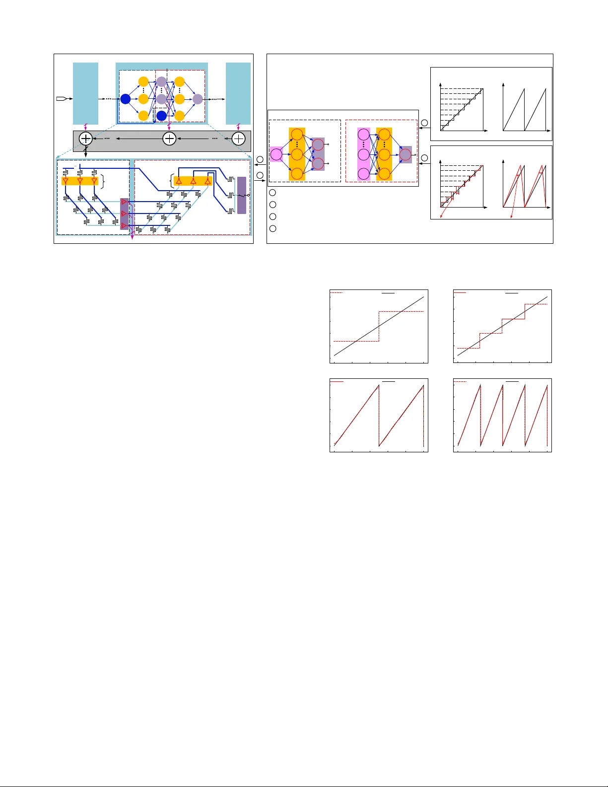
Neural Network-Inspired Analog-to-Digital Con version to Achie ve Super -Resolution with Lo w-Precision RRAM De vices W eidong Cao*, Liu Ke*, A yan Chakrabarti** and Xuan Zhang* * Department of ESE, ** Department of CSE, W ashington Univ ersity , St.louis, MO, USA Abstract — Recent works propose neural netw ork- (NN-) inspired analog-to-digital conv erters (NNADCs) and demon- strate their gr eat potentials in many emerging applications. These NN ADCs often rely on resistive random-access memory (RRAM) devices to realize the NN operations and require high-precision RRAM cells (6 ∼ 12-bit) to achieve a moderate quantization resolution (4 ∼ 8-bit). Such optimistic assumption of RRAM resolution, however , is not supported by fabrication data of RRAM arrays in large-scale production process. In this paper , we pr opose an NN-inspir ed super-r esolution ADC based on low-precision RRAM devices by taking the advantage of a co-design methodology that combines a pipelined hardware architectur e with a custom NN training framework. Results obtained from SPICE simulations demonstrate that our method leads to rob ust design of a 14-bit super -r esolution ADC using 3- bit RRAM de vices with impro ved power and speed performance and competitive figure-of-merits (FoMs). In addition to the linear uniform quantization, the proposed ADC can also sup- port configurable high-resolution nonlinear quantization with high con version speed and low conv ersion energy , enabling future intelligent analog-to-information interfaces f or near - sensor analytics and processing. I . I N T R O D U C T I O N Many emerging applications hav e posed new challenges for the design of conv entional analog-to-digital (A / D) con- verters (ADCs) [1]–[4]. For example, multi-sensor systems desire programmable nonlinear A / D quantization to maxi- mize the extraction of useful features from the raw analog signal, instead of directly performing uniform quantization by con ventional ADCs [3], [4]. This can alleviate the compu- tational burden and reduce the power consumption of back- end digital processing, which is the dominant bottleneck in intelligent multi-sensor systems. Howe ver , such flexible and configurable quantization schemes are not readily supported by conv entional ADCs with dedicated circuitry that has fixed con version references and thresholds. T o ov ercome this inherent limitation of con ventional ADCs, sev eral recent works [5]–[7] have introduced neural network-inspired ADCs (NN ADCs) as a novel approach to designing intelligent and flexible A / D interfaces. For instance, a learnable 8-bit NN ADC [7] is presented to approximate multiple quantization schemes where the NN weight parameters are trained off-line and can be config- ured by programming the same hardware substrate. Another example is a 4-bit neuromorphic ADC [6] proposed for general-purpose data conv ersion using on-line training by lev eraging the input amplitude statistics and application sen- sitivity . These NN ADCs are often b uilt on resistiv e random- access memory (RRAM) crossbar array to realize the basic NN operations, and can be trained to approximate the spe- cific quantization / con version functions required by dif ferent systems. Howe ver , a major challenge for designing such NN ADCs is the limited conductance / resistance resolution of RRAM devices. Although these NN ADCs optimistically assume that each RRAM cell can be precisely programmed with 6 ∼ 12-bit resolution, measured data from realistic fab- rication process suggest the actual RRAM resolution tends to be much lower (2 ∼ 4-bit) [8], [9]. Therefore, there exists a gap between the reality and the assumption of RRAM precision, yet lacks a design methodology to build super- resolution NN ADCs from lo w-precision RRAM devices. In this paper , we bridge this gap by introducing an NN- inspired design methodology that constructs super-resolution ADCs with lo w-precision RRAM devices. T aking adv antage of a co-design methodology that combines a pipelined hard- ware architecture with deep learning-based custom training framew ork, our method is able to achieve an NN-inspired ADC whose resolution far exceeds the precision of the underlying RRAM devices. The key idea of a pipelined architecture is that many consecuti ve low-resolution (1 ∼ 3- bit) quantization stages can be cascaded in a chain structure to obtain higher resolution. Since each stage now only needs to resolve 1 ∼ 3-bit, we can accurately train and instantiate it with low-precision RRAM devices to approximate the ideal quantization functions and residue functions. Key innov a- tions and contributions in this paper are as follow: • W e propose a co-design methodology lev eraging pipelined hardware architecture and custom training framew ork to achie ve super -resolution analog-to-digital con version that far exceeds the limited precision of the RRAM device. • W e systematically ev aluate the impacts of NN size and RRAM precision on the accuracy of NN-inspired sub-ADC and residue block and perform design space exploration to search for optimal pipelined stage con- figuration with balanced trade-of f between speed, area, and power consumption. • SPICE simulation results demonstrate that our proposed method is able to generate robust design of a 14-bit super-resolution NNADC using 3-bit RRAM devices. Comparisons with both the state-of-the-art ADCs and other NNADC designs reveal improv ed performance and competitiv e figure-of-merits (FoMs). • Our proposed ADC can also support configurable non- linear quantization with high-resolution, high con ver - sion speed, and low con version energy . I I . P R E L I M I N A R I E S A. RRAM Device, Cr ossbar Array and NN 1) RRAM device: A RRAM device is a passive two- terminal element with variable resistance and possesses many special advantages, such as small cell size (4 F 2 , F – the minimum feature size), excellent scalability ( < 10 nm ), faster read / write time ( < 10 ns ) and better endurance ( ∼ 10 10 cycles) than Flash devices [2], [10]. 2) RRAM cr ossbar array: RRAM devices can be orga- nized into various ultra-dense crossbar array architectures. Fig. 1(a) shows a passiv e crossbar array composed of two sub-arrays to realize bipolar weights without the use of power -hungry operational-amplifiers (op-amps) [7]. The relationship between the input voltage “vector” ( ~ V in ) and output voltage “vector” ( ~ V o ) can be expressed as V o ,j = P k W k,j · V in ,k + V off ,j . Here, k ( k ∈ { 1 , 2 , . . . , H } ) and j ( j ∈ { 1 , 2 , . . . , M } ) are the indices of input ports and output ports of the crossbar array . The weight W k,j can be represented by the subtraction of two conductances in upper ( U ) sub-array and lower ( L ) sub-array as W k,j = ( g U k,j − g L k,j ) / X , X = X k ( g U k,j + g L k,j ) . (1) Therefore, the RRAM crossbar array is capable of per- forming analog vector-matrix multiplication (VMM) and the parameters of the matrix rely on the RRAM resistance states. 3) Artificial NN: With the RRAM crossbar array , an NN shown in Fig. 1(b) can be implemented on such hardware substrate. Generally , the NN processes the data by ex ecuting the following operations layer-wise [17]: ~ y i + 1 = f ( W i,i + 1 · ~ x i + ~ b i + 1 ) . (2) Here, W i,i + 1 is the weight matrix to connect the layer i and layer ( i + 1 ) . f ( · ) is a nonlinear activ ation function (N AF). These basic NN operations, e.g., VMM and N AF , can be mapped to the RRAM crossbar array and CMOS inv erters shown in Fig. 1(a), where the voltage transfer characteristic (VTC) is used as an N AF [7]. B. NN-Inspir ed ADCs ADC can be viewed as a special case of classification problems which maps a continuous analog signal to a multi- bit digital code. An NN can be trained to learn this input- output relationship, and a hardware implementation of this NN can be instantiated in the analog and mixed-signal domain. This is the basic idea behind NN ADCs which imple- ments the learned NN on a hardware substrate to approximate the desired quantization functions for data con version: M X i = 1 2 i − 1 · b o ,i = round  V in − V min V max − V min × ( 2 M − 1 )  , (3) where, M is the resolution; V in is input analog signal and b o is the output digital codes; V min and V max are the minimum and maximum values of the scalar input signal V in . Since RRAM crossbar array provides a promising hardware substrate to build NNs, recent work has demonstrated sev eral NN ADCs based on RRAM devices [5]–[7]. Although the NN architectures adopted by these NN ADCs are various, they all ( b ) ( a ) u p p e r s u b - a r r a y l o w e r s u b - a r r a y S o u r c e l i n e B i t l i n e P i n , H V P i n , k V P i n , 1 V N i n , 1 V N i n , k V N i n , H V U k , j g L k , j g o , M V o , j V o , 1 V PN i n i n i n V ( V , V ) PN i n , k i n , k i n , k D D i n , k V V , V V V V T C i , i 1 i , 1 X i , 2 X i , 3 X i , n X i 1 , 1 b i 1 , 2 b i 1 , m b i 2 , 1 b i 2 , p b i 1 , i 2 ( b ) ( a ) u p p e r s u b - a r r a y l o w e r s u b - a r r a y S o u r c e l i n e B i t l i n e P i n , H V P i n , k V P i n , 1 V N i n , 1 V N i n , k V N i n , H V U k , j g L k , j g o , M V o , j V o , 1 V PN i n i n i n V ( V , V ) PN i n , k i n , k i n , k D D i n , k V V , V V V V T C i , i 1 i , 1 X i , 2 X i , 3 X i , n X i 1 , 1 b i 1 , 2 b i 1 , m b i 2 , 1 b i 2 , p b i 1 , i 2 ( b ) ( a ) u p p e r s u b - a r r a y l o w e r s u b - a r r a y S o u r c e l i n e B i t l i n e V T C , P i n H V , P i n k V ,1 P in V , N i n H V , N i n k V ,1 N in V , N kj g , P kj g , in X ,3 i X ,1 i X ,2 i X 1,  im b 1 , 2  i b 1 , 1  i b 2,  ip b 2 , 1  i b ,1  ii ω 1 , 2  ii ω , , , , ,    PN i n k i n k i n k D D i n k V V V V V  in V ( , ) PN i n i n VV (b) (a) uppe r sub-ar ray lower sub- a rra y Sou r c e line Bit line VTC , P in H V , P in k V ,1 P in V , N in H V , N in k V ,1 N in V , N kj g , P kj g , , , , ,    PN in k in k in k DD in k V V V V V  in V ( , ) PN in in VV i, n X i, 3 X i, 2 X i, 1 X i 1 , m b  i 1 , 2 b  i 1 , 1 b  i 2,p b  i 2, 1 b  i, i 1  ω i 1 , i 2  ω Fig. 1: (a) Hardware substrate to perform basic NN operations, where the passiv e crossbar array with two sub-arrays e xecutes VMM and the VTC of CMOS inv erter acts as NAF . (b) An example of NN. rely on a training process to learn the appropriate NN weights to approximate flexible quantization schemes that can be configured by programming the weights stored in RRAM conductance / resistance. Howe v er , existing NN ADCs [5]– [7] often exhibit modest conv ersion resolution (4 ∼ 8-bit) and in v ariably rely on optimistic assumption of the RRAM precision (6 ∼ 12-bit), which is not well substantiated by mea- surement data from realistic RRAM fabrication process [8], [9]. This resolution limitation se verely constrains the appli- cation of NN ADCs in emerging multi-sensor systems that require high-resolution ( > 10-bit) A / D interfaces for feature extraction and near-sensor processing [1], [3], [4]. C. Pipelined ADCs Pipelined architecture is a well-established ADC topology to achieve high sampling rate and high resolution with low- resolution quantization stages [11]. Fig. 2(a) illustrates a typical pipelined ADC with M stages whose resolution RESO can be achieved by concatenating N i -bit of each stage with digital combiner: RESO = P M i = 1 N i . Note that N i is usually ≤ 4 and not necessarily identical in all stages. As the Fig. 2(a) illustrates, an arbitrary stage- i contains two sub- blocks: a sub-ADC and a residue. The sub-ADC resolves N i -bit binary codes D N i from input residue r i − 1 , while the residue part amplifies the subtraction between the input residue r i − 1 and the analog output of sub-ADC by 2 N i to generate the output residue r i for next stage. This process can be expressed as a simple function: r i = [ r i − 1 − REF ( D N i )] · 2 N i . (4) Here, REF ( D N i ) is the analog output of sub-DA C that depends on D N i . For example, assuming r i − 1 ∈ [ 0 , V DD ] and N i = 1, then REF ( 0 ) = 0 and REF ( 1 ) = V DD / 2; and Fig. 2(b) shows the corresponding residue function. T o understand the basic working principle of pipelined ADCs, we use a 4-bit pipelined ADC with four 1-bit stages in Fig. 2(c) as an example. Assuming the initial analog input is 0 . 7 V ( V DD = 1 V ), then the first stage will output “1”— a digital code, and “0 . 4 V ”— an analog residue according to Eq. (4) which will be processed by the following stage in the same way as initial analog input. Finally , we can obtain 4-bit outputs 1011, which is the quantization of 0 . 7 V (0 . 7 / 1 = 11 . 2 / 2 4 ≈ 11 / 2 4 ). This example also shows that a higher resolution (4-bit) can indeed be constructed with low-precision (1-bit) stages in a pipelined ADC. V IN G e n e r a l P i p e l i n e d A D C A r c h i t e c t u r e L S B S t a g e - 1 . . . S t a g e - M N 1 - b i t N M - b i t . . . M S B D i g i t a l C o m b i n e r S t a g e - i S t a g e - M V IN D O U T S u p e r - r e s o A D C A r c h i t e c t u r e F l a sh A D C R e si d u e p a r t N i 1 i1 r i r 1 r M1 r r i ( a ) H a r d w a r e S u b s t r a t e o f S t a g e - i R e si d u a l p a r t ( b ) N i ... ... r i 1 N i ... ... ... ... ... F l a sh A D C S / H i1 r S t a g e - 1 - b i t 1 N - b i t i N M N - b i t 1 2 M 1 M N N . . . N N - b i t N i 1 ... V IN O f f l i n e T r a i n i n g M o d e l o f S t a g e - i F l a sh A D C V IN N i 1 i r - b i t i N R e si d u a l p a r t R e s i d u e 0 V in V DD V DD Q u a n t i z a t i o n o u t p u t s 0 V in L i n e a r U n i f o r m V DD G r o u n d T r u t h D a t a s e t s T r a i n i n g O b j e c t i v e R e s i d u e 0 V in V DD V DD M i n i m i z e co st b a s e d o n d i scre p a n cy b e t w e e n t ru e a n d p re d i ct e d b i t s 0 V in Q u a n t i z a t i o n o u t p u t s V DD M i n i m i z e co st b a s e d o n d i scre p a n cy b e t w e e n t ru e a n d p re d i ct e d re si d u e O p ti m a l T r a i n i n g F l o w 2 4 1 3 e st a b l i sh l e a r n i n g o b j e ct i ve g e n e r a t e d a t a se t s a n d t r a i n t h r o u g h b a ckp r o p a g a t i o n i n st a n t i a t e d e si g n p a r a m e t e r s m o d e l h a r d w a r e su b st r a t e co n st r a i n t s 1 2 3 4 ( c ) Q u a n t i z a t i o n f u n c t i o n R e s i d u a l f u n c t i o n ( d ) ( e ) T r a i n i n g F r a m e w o r k 1 F , 1 b 1 F , 2 b 1 F , H b 1 R , 1 b 1 R , 2 b 1 R , H b 2 F , 1 b i 2 F , N b 2 R , 1 b O p ti m a l H a r d w a r e A r c h i te c tu r e 1 r i1 r i r M1 r R e s i d u e 0 V in V DD V DD s u b - A D C s u b - D A C D i g i t a l C o m b i n e r S t a g e - i V IN 1 2 M ( N N . . . N ) - b i t D O U T G e n e r a l P i p e l i n e d A D C A r c h i t e c t u r e L S B A D C R e s i d u e S t a g e - 1 . . . S t a g e - M N 1 - b i t N i - b i t N M - b i t ... M S B ... ... 1 r i1 r i N 2 i r M1 r r i 0 r i - 1 V DD V DD R e s i d u e r i 0 r i - 1 V DD V DD R e s i d u e 0 . 7 V 0 . 5 V ( m i d ) 0 . 4 V N i - b i t S t a g e - i s u b - A D C s u b - D A C A D C R e s i d u e i N 2 N i - b i t i1 r i r 1 V 0 .1 0 . 8 V 0 . 6 V . . . 0 . 1 G e n e r a l P i p e l i n e d A D C A r c h i t e c t u r e 1 2 3 4 ( a ) ( c ) 1 0 1 1 ( b ) V IN L S B S t a g e - 1 . . . S t a g e - M N 1 - b i t N M - b i t . . . M S B 1 r i1 r i r M1 r r i 0 r i - 1 V DD V DD R e s i d u e f u n c t i o n 0 . 7 V 0 . 5 V ( m i d ) 0 . 4 V N i - b i t S t a g e - i s u b - A D C s u b - D A C A D C R e s i d u e i N 2 N i - b i t i1 r i r 1 V 0 .1 0 . 8 V 0 . 6 V . . . 0 . 1 G e n e r a l P i p e l i n e d A D C A r c h i t e c t u r e 1 2 3 4 ( a ) ( c ) 1 0 1 1 ( b ) S t a g e V IN L S B S t a g e - 1 . . . S t a g e - M N 1 - b i t N M - b i t . . . M S B r i 0 r i - 1 V DD V DD R e s i d u e f u n c t i o n 0 . 7 V 0 . 5 V ( m i d ) 0 . 4 V N i - b i t S t a g e - i s u b - A D C s u b - D A C S u b - A D C R e s i d u e 1 V 0 . 8 V 0 . 6 V . . . 0 . 1 G e n e r a l P i p e l i n e d A D C A r c h i t e c t u r e 1 2 3 4 ( a ) ( c ) 1 0 1 1 ( b ) S t a g e 1  i r 2 i N i r N i - b i t 1 r 1  i r i r 1  M r 0 . 1  s u b - A D C V IN LSB Stage-1 ... N 1 -bit N M -bit ... MSB r i 0 r i-1 V DD V DD Residue fu nction 0.7 V 0.5 V (mid) 0.4 V N i -bit Stage-i sub-A DC sub- DAC Sub- ADC Res idue 1 V 0.8 V 0.6 V ... 0.1 Gen eral P i pelined ADC Arc hitectu re 1 2 3 4 (a) (c) 1 0 1 1 (b) Stage 1  i r 2 i N i r N i -bit 1 r 1  i r i r 1  M r 0.1  sub- ADC Stage-M Fig. 2: (a) General architecture of pipelined ADC. (b) An example of residue function when N i = 1. (c) A quantization example of a 4-bit pipelined ADC with four 1-bit stages. I I I . C O - D E S I G N M E T H O D O L O G Y A. Har dwar e Substrate 1) Pipelined ar chitectur e: The observ ation from tradi- tional pipelined ADCs motiv ates us to extend such archi- tecture to NNADC to enhance its resolution beyond the limit of RRAM precision. The overall hardware architec- ture for the proposed high-resolution NN ADC is presented in Fig. 3(a), where a pipelined architecture composed of cascaded con version stages is adopted in the design. This pipelined architecture brings two direct benefits. First, each stage in the proposed NN ADC no w only needs to resolve 1 ∼ 3-bit quantization, which is well within the precision limit of current RRAM fabrication process [8], [9] and can be easily achie ved with the automated design methodology introduced in previous work [7]. Second, although many cascading stages are needed, there only exist three distinct low-resolution configurations to choose from for each stage, namely N i = 1 , 2 , 3. This allows us to simplify the design process by focusing on optimizing the sub-block design of each stage with dif ferent resolutions. The full pipelined system can then be assembled by iterating through different combinations of the sub-blocks with different resolutions. 2) Low-r esolution NNADC stage: For stage- i in the pro- posed NN ADC, we use a fiv e-layer NN to implement the sub-ADC and the residue block. The five-layer NN can be decomposed into two three-layer sub-blocks, and each of them can be mapped into the corresponding sub-ADC and residue in Fig. 2(a). The cornerstone of this mapping methodology is the uni versal approximation theorem that a feed-forward three-layer NN with a single hidden layer can approximate arbitrary complex functions [13]. W e use the RRAM crossbar array and CMOS in verter illustrated in Fig. 1(a) as the hardware substrate to design the sub-blocks of each stage. As Fig. 3(b) shows, for the sub-ADC, the input analog signal represents the single “place holder” neuron in MLP’ s input layer . Therefore, the weight matrix dimensions are H F,i × 1 between the hidden and the input layer , and H F,i × S i between the hidden and the output layer , assuming there are H F,i and S i neurons in the hidden and output layer . Here, we use a redundant “smooth” S i → N i encoding method to replace the standard N i -bit binary encoding with S i bits ( S i > N i ) according to pre vious work [7], as it improv es the training accuracy and reduces hidden layer size of the sub-ADC. For example, we use 3 → 2 smooth codes to train a 2-bit sub-ADC with 3-bit smooth codes as output in Fig. 4(b). For the residue, there are (1 + S i ) input neurons (one analog input and S i -bit smooth digital codes from the proceeding sub-ADC block), and only one analog output neuron; therefore, the weight matrix dimensions are H R,i × ( 1 + S i ) between the hidden and the input layer and H R,i × 1 between the hidden and the output layer , assuming there are H R,i hidden neurons. The sampling / hold (S / H) circuits [18] are used in the output layer to drive the next stage. Since the op-amps in Fig. 2(a) are eliminated in the NN-inspired design of residue circuit, considerable power saving can be obtained from each stage. B. T r aining F ramework 1) T r aining overview: W e propose a training framework that accurately captures the circuit-level behavior of the hardware substrate in its mathematical model and is able to learn the robust NNs and its associated hardware design parameters (i.e., RRAM conductance) to approximate the sub-ADC and residue for each stage. The training frame- work incorporates two important features. First, we employ collaborativ e training for the two sub-blocks in each stage. The sub-ADC is initially trained to approximate the ideal quantization function with high-fidelity , then its digital out- puts and original analog input are directly fed to the residue block for the residue training. This collaborativ e training flow can ef fecti vely minimize the discrepancy between the circuit artifacts and the ideal conv ersion at each stage. Second, non- idealities of devices, such as process, voltage and temperature (PVT) variations of the CMOS device and limited precision of the RRAM devices, can be incorporated into training to make the proposed NNADC robust to these defects [14]. This is another advantage of the proposed NN ADC ov er traditional ADC designs, where even with delicate calibration techniques, the non-idealities cannot be fully mitigated [11]. 2) T r aining steps: The detailed training flow is shown in Fig. 3(b), which consists of four steps. W e focus on de- scribing the training steps for the residue block, as we adopt similar sub-ADC training method that has been elaborated in previous work [7], [14]. Step 1  : establish learning objectiv e. For the residue circuit, its output is an analog v alue; therefore, the hardware substrate can be modeled as a three-layer NN with a “place- holder” output neuron: ˜ h i = L 1 ( r i − 1 , D S i ; θ 1 ,i ) , r i = L 2 ( h i ; θ 2 ,i ) . (5) Here, h i = σ VTC,i ( ˜ h i ) . D S i indicates the digital output of the ADC (“1” means V DD , and “0” means GND), and r i − 1 is the scalar residue input of stage- i ; ˜ h i denote the outputs of the first crossbar layer , which are modeled as a linear function L 1 of r i − 1 and D S i , with learnable parameters θ 1 ,i = { W 1 , V 1 } corresponding to RRAM crossbar array conductances. Each of these voltages is passed through an in verter (shown in Fig. 1(a)), whose input-output relationship is modeled by the nonlinear function σ VTC,i ( · ) , to yield the vector h i . The linear function L 2 models the second layer of the crossbar to ( b ) N i 1 ... V IN O f f l i n e T r a i n i n g M o d e l o f S t a g e - i F l a sh A D C V IN N i 1 i r - b i t i N R e si d u a l p a r t R e s i d u e 0 V in V DD V DD Q u a n t i z a t i o n o u t p u t s 0 V in L i n e a r U n i f o r m V DD G r o u n d T r u t h D a t a s e t s T r a i n i n g O b j e c t i v e R e s i d u e 0 V in V DD V DD M i n i m i z e co st b a s e d o n d i scre p a n cy b e t w e e n t ru e a n d p re d i ct e d b i t s 0 V in Q u a n t i z a t i o n o u t p u t s V DD M i n i m i z e co st b a s e d o n d i scre p a n cy b e t w e e n t ru e a n d p re d i ct e d re si d u e 2 4 1 3 e st a b l i sh l e a r n i n g o b j e ct i ve g e n e r a t e d a t a se t s a n d t r a i n t h r o u g h b a ckp r o p a g a t i o n i n st a n t i a t e d e si g n p a r a m e t e r s m o d e l h a r d w a r e su b st r a t e co n st r a i n t s 1 2 3 4 ( c ) Q u a n t i z a t i o n f u n c t i o n R e s i d u a l f u n c t i o n ( d ) ( e ) T r a i n i n g F r a m e w o r k 1 F , 1 b 1 F , 2 b 1 F , H b 1 R , 1 b 1 R , 2 b 1 R , H b 2 F , 1 b i 2 F , N b 2 R , 1 b ... ... S u b - A D C ... ... 1 S i r i S / H i1 r H a r d w a r e S u b s t r a t e o f S t a g e - i R e si d u e ci r cu i t ... H F , i H R , i ... ... D i g i t a l C o m b i n e r S t a g e - i S t a g e - M V IN D O U T S u b - A D C R e si d u e ci r cu i t S i 1 i1 r i r 1 r M1 r ( a ) S t a g e - 1 - b i t 1 N - b i t i N M N - b i t 1 2 M 1 M N N . . . N N - b i t H a r d w a r e A r c h i t e c t u r e N i 1 ... V IN O f f l i n e T r a i n i n g M o d e l o f S t a g e - i F l a sh A D C V IN N i 1 i r - b i t i N R e si d u a l p a r t R e s i d u e 0 V in V DD V DD Q u a n t i z a t i o n o u t p u t s 0 V in L i n e a r U n i f o r m V DD G r o u n d T r u t h D a t a s e t s T r a i n i n g O b j e c t i v e R e s i d u e 0 V in V DD V DD M i n i m i z e co st b a s e d o n d i scre p a n cy b e t w e e n t ru e a n d p re d i ct e d b i t s 0 V in Q u a n t i z a t i o n o u t p u t s V DD M i n i m i z e co st b a s e d o n d i scre p a n cy b e t w e e n t ru e a n d p re d i ct e d re si d u e 2 4 1 3 e st a b l i sh l e a r n i n g o b j e ct i ve g e n e r a t e d a t a se t s a n d t r a i n t h r o u g h b a ckp r o p a g a t i o n i n st a n t i a t e d e si g n p a r a m e t e r s m o d e l h a r d w a r e su b st r a t e co n st r a i n t s 1 2 3 4 ( b ) Q u a n t i z a t i o n f u n c t i o n R e s i d u e f u n c t i o n 1 F , 1 b 1 F , 2 b 1 F , H b 1 R , 1 b 1 R , 2 b 1 R , H b 2 F , 1 b i 2 F , N b 2 R , 1 b T r a i n i n g F r a m e w o r k D i g i t a l C o m b i n e r S t a g e - i S t a g e - M V IN D OU T S u b - A D C R e si d u e ci r cu i t S i 1 i1 r i r 1 r M1 r S t a g e - 1 - b i t 1 N - b i t i N M N - b i t H a r d w a r e A r c h i te c tu r e ... ... S u b - A D C ... ... 1 S i r i S / H i1 r R e si d u e ci r cu i t ... H F , i H R , i ... ... ... - b i t M i i1 N ( a ) S i 1 ... V IN O f f l i n e T r a i n i n g M o d e l o f S t a g e - i S u b - A D C V IN S i 1 i r - b i t R e si d u e R e s i d u e 0 V in V DD V DD Q u a n t i z a t i o n o u t p u t s 0 V in L i n e a r U n i f o r m V DD G r o u n d T r u t h D a t a s e t s T r a i n i n g O b j e c t i v e R e s i d u e 0 V in V DD V DD M i n i m i z e co st b a s e d o n d i scre p a n cy b e t w e e n t ru e a n d p re d i ct e d b i t s 0 V in Q u a n t i z a t i o n o u t p u t s V DD M i n i m i z e co st b a s e d o n d i scre p a n cy b e t w e e n t ru e a n d p re d i ct e d re si d u e 2 4 1 3 e st a b l i sh l e a r n i n g o b j e ct i ve g e n e r a t e d a t a se t s a n d t r a i n t h r o u g h b a ckp r o p a g a t i o n i n st a n t i a t e d e si g n p a r a m e t e r s m o d e l h a r d w a r e su b st r a t e co n st r a i n t s 1 2 3 4 ( b ) Q u a n t i z a t i o n f u n c t i o n R e s i d u e f u n c t i o n 1 F , 1 b 1 F , 2 b 1 F , H b 1 R , 1 b 1 R , 2 b 1 R , H b 2 F , 1 b 2 R , 1 b T r a i n i n g F r a m e w o r k D i g i t a l C o m b i n e r S t a g e - i S t a g e - M V IN D OU T S u b - A D C R e si d u e S i 1 i1 r i r 1 r M1 r S t a g e - 1 - b i t 1 N - b i t i N M N - b i t H a r d w a r e A r c h i te c tu r e ... ... S u b - A D C ... ... 1 S i r i S / H i1 r R e si d u e ... H F , i H R , i ... ... ... - b i t M i i1 N ( a ) i 2 F , S b S i S i 1 ... V IN O f f l i n e T r a i n i n g M o d e l o f S t a g e - i S u b - A D C V IN S i 1 i r - b i t R e si d u e R e s i d u e 0 V in V DD V DD Q u a n t i z a t i o n o u t p u t s 0 V in L i n e a r U n i f o r m V DD G r o u n d T r u t h D a t a s e t s T r a i n i n g O b j e c t i v e R e s i d u e 0 V in V DD V DD M i n i m i z e co st b a s e d o n d i scre p a n cy b e t w e e n t ru e a n d p re d i ct e d b i t s 0 V in Q u a n t i z a t i o n o u t p u t s V DD M i n i m i z e co st b a s e d o n d i scre p a n cy b e t w e e n t ru e a n d p re d i ct e d re si d u e 2 4 1 3 e st a b l i sh l e a r n i n g o b j e ct i ve g e n e r a t e d a t a se t s a n d t r a i n t h r o u g h b a ckp r o p a g a t i o n i n st a n t i a t e d e si g n p a r a m e t e r s m o d e l h a r d w a r e su b st r a t e co n st r a i n t s 1 2 3 4 ( b ) Q u a n t i z a t i o n f u n c t i o n R e s i d u e f u n c t i o n 1 F , 1 b 1 F , 2 b 1 F , H b 1 R , 1 b 1 R , 2 b 1 R , H b 2 F , 1 b 2 R , 1 b T r a i n i n g F r a m e w o r k D i g i t a l C o m b i n e r S t a g e - i S t a g e - M V IN D OU T S u b - A D C R e si d u e S i 1 i1 r i r 1 r M1 r S t a g e - 1 - b i t 1 N - b i t i N M N - b i t H a r d w a r e A r c h i t e c t u r e ... ... S u b - A D C ... ... 1 S i r i S / H i1 r R e si d u e ... H F , i H R , i ... ... ... - b i t M i i1 N ( a ) i 2 F , S b S i S i 1 ... V IN O f f l i n e T r a i n i n g M o d e l o f S t a g e - i S u b - A D C V IN S i 1 i r - b i t R e si d u e R e s i d u e 0 V in V DD V DD Q u a n t i z a t i o n o u t p u t s 0 V in L i n e a r U n i f o r m V DD G r o u n d T r u t h D a t a s e t s T r a i n i n g O b j e c t i v e R e s i d u e 0 V in V DD V DD M i n i m i z e co st b a s e d o n d i scre p a n cy b e t w e e n t ru e a n d p re d i ct e d b i t s 0 V in Q u a n t i z a t i o n o u t p u t s V DD M i n i m i z e co st b a s e d o n d i scre p a n cy b e t w e e n t ru e a n d p re d i ct e d re si d u e 2 4 1 3 e st a b l i sh l e a r n i n g o b j e ct i ve g e n e r a t e d a t a se t s a n d t r a i n t h r o u g h b a ckp r o p a g a t i o n i n st a n t i a t e d e si g n p a r a m e t e r s m o d e l h a r d w a r e su b st r a t e co n st r a i n t s 1 2 3 4 Q u a n t i z a t i o n f u n c t i o n R e s i d u e f u n c t i o n 1 F , 1 b 1 F , 2 b 1 F , H b 1 R , 1 b 1 R , 2 b 1 R , H b 2 F , 1 b 2 R , 1 b T r a i n i n g F r a m e w o r k D i g i t a l C o m b i n e r S t a g e - i S t a g e - M V IN D OU T S u b - A D C R e si d u e S i 1 i1 r i r 1 r M1 r S t a g e - 1 - b i t 1 N - b i t i N M N - b i t H a r d w a r e A r c h i t e c t u r e ... ... S u b - A D C ... ... 1 S i r i S / H i1 r R e si d u e ... H F , i H R , i ... ... ... - b i t M i i1 N ( a ) i 2 F , S b S i ( b ) S i 1 ... V IN Offline Training Model of Stage-i Sub-ADC V IN S i 1 i r -bit Residue Res idue 0 V in V DD V DD Quan t izat io n output s 0 V in Linea r Uniform V DD Ground Truth Datasets Training Objective Res idue 0 V in V DD V DD M inim iz e co st bas ed o n discrepancy between tru e and predicted bits 0 V in Quan t izat io n output s V DD M inim iz e co st bas ed o n discrepancy between tru e and predicted residue 2 4 1 3 establish learning objective generate datasets and train through backpropaga t i on instantiate design parameters model hardware substrate constraints 1 2 3 4 Quan t izat io n function R esidue f unc ti on 1 F, 1 b 1 F,2 b 1 F,H b 1 R, 1 b 1 R,2 b 1 R,H b 2 F, 1 b 2 R, 1 b Trai ning F ram ework Digital Combiner Stage-i Stage-M V IN D OUT Sub-ADC Residue S i 1 i r 1 r Stage-1 -bit 1 N -bit i N M N -bit H ardwa re Arc hitect ure ... ... Sub-ADC ... ... 1 S i r i S/H i 1 r Residue ... H F,i H R,i ... ... ... (a) i 2 F,S b S i (b) -bit M i i1 N   i1 r  M1 r  Fig. 3: Proposed co-design frame work for the super-resolution NNADC. (a) Pipelined architecture for the proposed NNADC. (b) Of f-line training model of each stage- i . Proposed training framework takes ground truth datasets as inputs during of f-line training to find the optimal weights and deri ve the RRAM resistances to minimize cost function and best approximate ideal quantization function and residue function. produce the output residue r i for next stage, with learnable parameters θ 2 ,i = { W 2 , V 2 } . The learning objectiv e is to find optimal values for the parameters { θ 1 ,i , θ 2 ,i } such that for all v alues of r i − 1 in the input range, the circuit yields corresponding residue r i that are equal or close to the desired “ground truth” r GT in Eq. (4). T o achieve this aim, we define a cost function C ( r i , r GT ) to measure the discrepancy between predicted r i and true r GT based on the mean-square loss: C ( r i , r GT ) = X j [ r GT ( j ) − r i ( j )] 2 . (6) Step 2  : model hardware constraints. Hardware constraints come from three aspects: CMOS neuron PVT v ariations, limited precision of RRAM device, and passiv e crossbar array . T o reflect these hardware constraints, we first group all VTCs obtained by Monte Carlo simulations in A VTC using the technology specification in Section IV -A. Meanwhile, we control the precision of weight with A R -bit during the training. Finally , we let the summation of all elements (absolute value) in each column (“0”) of W 1 , 2 be < 1: X ( abs ( W 1 ) , 0 ) < 1 ; X ( abs ( W 2 ) , 0 ) < 1 , (7) to reflect the weights constraints in Eq. (1). Step 3  : hardware-oriented training. W e initialize the parameters { θ 1 ,i , θ 2 ,i } randomly , and update them itera- tiv ely based on gradients computed on mini-batches of { ( r i − 1 , D N i , r GT ) } pairs randomly sampled from the input range. T o incorporate the hardware constraints in step 2  into training, we let each neuron j in Eq. (5) randomly pick up a VTC from A VTC during training: σ j VTC,i = A VTC [ randint ( N )] , j = 1 , 2 , ..., H R,i . (8) W e then periodically clip all values of W 1 between [ − 1 / ( 1 + N i ) , 1 / ( 1 + N i )] , as well as W 2 between [ − 1 /H R,i , 1 /H R,i ] to satisfy Eq. (7). Step 4  : instantiate conductance values. W e adopt the same instantiation method based on pre vious work [7], which is prov en to always find a set of equiv alent conductances from the trained weights and biases to map to the RRAM ( a ) ( b ) 1 . 0 0 . 8 0 . 6 0 . 4 0 . 2 0 . 0 0 . 0 0 . 2 0 . 4 0 . 6 0 . 8 1 . 0 In p u t ( V ) Res i d u e ( V ) I d e a l re si d u e T ra i n e d re si d u e A m p l i tu d e ( V ) 1 . 0 0 . 8 0 . 6 0 . 4 0 . 2 0 . 0 0 . 0 0 . 2 0 . 4 0 . 6 0 . 8 1 . 0 0 1 0 . 0 0 . 2 0 . 4 0 . 6 0 . 8 1 . 0 A m p l i tu d e ( V ) 1 . 0 0 . 8 0 . 6 0 . 4 0 . 2 0 . 0 In p u t ( V ) In p u t ( V ) 00 01 10 11 O rg i n a l R e co n st ru ct e d O rg i n a l R e co n st ru ct e d 1 . 0 0 . 8 0 . 6 0 . 4 0 . 2 0 . 0 0 . 0 0 . 2 0 . 4 0 . 6 0 . 8 1 . 0 In p u t ( V ) Re s i d u e ( V ) I d e a l re si d u e T ra i n e d re si d u e N i = 1 , 1 - b i t s t a g e N i = 2 , 2 - b i t s t a g e S u b - ADC R e s i d u e S u b - ADC R e s i du e (a) (b) 1.0 0.8 0.6 0.4 0.2 0.0 0.0 0.2 0.4 0.6 0.8 1.0 Input (V) Residue (V) Ideal residue Trained residue Amplitude (V) 1.0 0.8 0.6 0.4 0.2 0.0 0.0 0.2 0.4 0.6 0.8 1.0 0 1 0.0 0.2 0.4 0.6 0.8 1.0 Amplitu d e (V) 1.0 0.8 0.6 0.4 0.2 0.0 Input (V ) Input (V ) 00 01 10 11 Orginal Reconstructed Orginal Reconstructed 1.0 0.8 0.6 0.4 0.2 0.0 0.0 0.2 0.4 0.6 0.8 1.0 Input (V) Residue (V) Ideal residue Trained residue N i =1 , 1-bit stage N i =2 , 2-bit stage Sub-ADC Residue Sub-ADC Residue Fig. 4: Illustrations of trained sub-ADC and residue functions for a pipeline stage with different resolution. (a) 1-bit stage ( N i = 1). (b) 2-bit stage ( N i = 2). devices in the hardware substrate. After this, we perturb each resistance R by: R ← R · e θ ; θ ∼ N ( 0 , σ 2 ) , (9) to e valuate the robustness of the NN model to the stochastic variation of RRAM resistance [2]. C. Examples of T r ained Sub-ADC and Residue Fig. 4 illustrates the SPICE simulation of different trained stages with the proposed training frame work. The sub-ADC and the residue in Fig. 4(a) are trained through a 1 × 3 × 2 NN and a 3 × 5 × 1 NN respectively by setting N i = 1, while the sub-ADC and the residue in Fig. 4(b) are trained through a 1 × 4 × 3 NN and a 4 × 7 × 1 NN by setting N i = 2. In both figures, we use 3-bit RRAM and set σ = 0 . 05 in Eq. (9) for ev aluation. The comparison between the trained function and the ideal function shows that each stage with low-precision RRAM can accurately approximate the ideal stage function with the aid of the proposed training framew ork. I V . E X P E R I M E N TA L R E S U LT S A. Experimental Methodology 1) T r aining configur ation: W e set N i = 1 , 2 , 3 to get three distinct resolution configurations in each pipeline stage in our experiments. For each stage, we train different NN models and each NN model is trained via stochastic gradient descent with the Adam optimizer using T ensorFlow [15]. The weight precision A R during training is set to be 1 ∼ 7-bit. The batch size is 4096, and the projection step is performed every 256 iterations. W e train for a total of 2 × 10 4 iterations for each sub-ADC model and residue model, varying the learning rate from 10 − 3 to 10 − 4 across the iterations. 2) T echnolo gy model: W e use the HfO x -based RRAM device model to simulate the crossbar array [16]. W e set the resistance stochastic variation σ = 0 . 05, since it is a moder- ate variation based on the e valuations from prior work [17]. The transistor model is based on a standard 130 nm CMOS technology . The inv erters, output comparators, and transistor switches in the RRAM crossbars are simulated with the 130nm model using Cadence Spectre. The VTC group A VTC is obtained by running 100 times Monte Carlo simulations. The simulation results presented in the following section are all based on SPICE simulation. 3) Metric of training accuracy: The trained accuracy of the sub-ADC / proposed NNADC is represented by the effecti v e number of bits (ENOB)–a metric to ev aluate the effecti v e resolution of an ADC. W e report ENOB based on its standard definition ENOB = (SNDR-1.76) / 6.02, where the signal to noise and distortion ratio (SNDR) is measured from the sub-ADC’ s / proposed NNADC’ s output spectrum. The training accuracy of the residue circuit is represented by the mean-square error (MSE) between predicted residue function and ideal residue function. W e report the MSE based on 2048 uniform sampling points in the full range of input [ 0 , V DD ] . B. Sub-block Evaluations 1) Resolution and r obustness: T o find a robust design for each stage, we study the relationship between the trained accuracy and RRAM precision of each sub-block with dif- ferent NN sizes at a fixed stochastic v ariation. For these experiments, we first incorporate both CMOS PVT v ariations and limited precision of RRAM de vice into training, and then instantiate sev eral batches of 100-run Monte Carlo simulations with a resistance variation σ = 0 . 05 in Eq. (9), and finally compute the median accuracy of each model. W e plot the trends in Fig. 5. Generally , an ( N i + 1 ) - bit RRAM precision is enough to train an NN model to accurately approximate an N i -bit sub-ADC, which confirms the conclusion in previous work [7]. Particularly , larger size NN models with more hidden neurons can even accu- rately approximate an N i -bit sub-ADC with N i -bit RRAM precision. Similar conclusions can also be made from the trained performance of residue circuits. As the Fig. 5(b) shows, an ( N i + 2 ) -bit RRAM precision is enough to train an NN model to accurately approximate a residue circuit. Moreov er , a larger size NN with more hidden layer neurons ( b ) ( a ) MSE 1 2 3 4 5 6 7 MSE R R AM p re ci si o n ( b i t s ) 3 - b i t 1 2 3 4 5 6 7 MSE R R AM p re ci si o n ( b i t s ) 4 - b i t 1 2 3 4 5 6 7 R R AM p re ci si o n ( b i t s ) 5 - b i t R e s i du e E v a l ua t i on 3 6 1  3 5 1  3 4 1  4 7 1  4 6 1  4 5 1  5 7 1  5 6 1  5 5 1  0 10 1 10  2 10  3 10  4 10  0 10 1 10  2 10  3 10  4 10  0 10 1 10  2 10  3 10  4 10  1  i N 2  i N 3  i N 1 2 3 4 5 0 . 5 1 . 0 1 . 5 EN O B ( b i t s ) R R AM p re ci si o n ( b i t s ) R R AM p re ci si o n ( b i t s ) 1 2 3 4 5 0 . 5 1 . 0 1 . 5 2 . 0 2 . 5 3 . 0 3 . 5 EN O B ( b i t s ) 1 2 3 4 5 0 0 . 5 1 . 0 1 . 5 2 . 0 2 . 5 EN O B ( b i t s ) R R AM p re ci si o n ( b i t s ) 2 - b i t 3 - b i t 4 - b i t S u b - A D C E v a l u a t i o n 1  i N 2  i N 3  i N 1 4 2  1 3 2  1 2 2  1 4 3  1 3 3  1 2 3  1 4 4  1 3 4  1 2 4  ( b ) ( a ) MSE 1 2 3 4 5 6 7 MSE R R AM p re ci si o n ( b i t s ) 3 - b i t 1 2 3 4 5 6 7 MSE R R AM p re ci si o n ( b i t s ) 4 - b i t 1 2 3 4 5 6 7 R R AM p re ci si o n ( b i t s ) 5 - b i t R e s i d u e E v a l u a t i o n 3 6 1  3 5 1  3 4 1  4 7 1  4 6 1  4 5 1  5 7 1  5 6 1  5 5 1  0 10 1 10  2 10  3 10  4 10  0 10 1 10  2 10  3 10  4 10  0 10 1 10  2 10  3 10  4 10  1  i N 2  i N 3  i N 1 2 3 4 5 0 . 5 1 . 0 1 . 5 EN O B ( b i t s ) R R AM p re ci si o n ( b i t s ) R R AM p re ci si o n ( b i t s ) 1 2 3 4 5 0 . 5 1 . 0 1 . 5 2 . 0 2 . 5 3 . 0 3 . 5 EN O B ( b i t s ) 1 2 3 4 5 0 0 . 5 1 . 0 1 . 5 2 . 0 2 . 5 EN O B ( b i t s ) R R AM p re ci si o n ( b i t s ) 2 - b i t 3 - b i t 4 - b i t S u b - A D C E v a l ua t i on 1  i N 2  i N 3  i N 1 4 2  1 3 2  1 2 2  1 4 3  1 3 3  1 2 3  1 4 4  1 3 4  1 2 4  ( b ) ( a ) MSE 1 2 3 4 5 6 7 MSE R R AM p re ci si o n ( b i t s ) 3 - b i t 1 2 3 4 5 6 7 MSE R R AM p re ci si o n ( b i t s ) 4 - b i t 1 2 3 4 5 6 7 R R AM p re ci si o n ( b i t s ) 5 - b i t R e s i d u e E v a l u a t i o n 3 6 1  3 5 1  3 4 1  4 7 1  4 6 1  4 5 1  5 7 1  5 6 1  5 5 1  0 10 1 10  2 10  3 10  4 10  0 10 1 10  2 10  3 10  4 10  0 10 1 10  2 10  3 10  4 10  1  i N 2  i N 3  i N 1 2 3 4 5 0 . 5 1 . 0 1 . 5 EN O B ( b i t s ) R R AM p re ci si o n ( b i t s ) R R AM p re ci si o n ( b i t s ) 1 2 3 4 5 0 . 5 1 . 0 1 . 5 2 . 0 2 . 5 3 . 0 3 . 5 EN O B ( b i t s ) 1 2 3 4 5 0 0 . 5 1 . 0 1 . 5 2 . 0 2 . 5 EN O B ( b i t s ) R R AM p re ci si o n ( b i t s ) 2 - b i t 3 - b i t 4 - b i t S ub - A D C E v a l u a t i o n 1  i N 2  i N 3  i N 1 4 2  1 3 2  1 2 2  1 4 3  1 3 3  1 2 3  1 4 4  1 3 4  1 2 4  (b) (a) MSE 1 2 3 4 5 6 7 MSE RRAM precision (bits) 3-bit 1 2 3 4 5 6 7 MSE RRAM precision (bits) 4-bit 1 2 3 4 5 6 7 RRAM precision (bits) 5-bit Residue Evaluation 3 6 1  3 5 1  3 4 1  4 7 1  4 6 1  4 5 1  5 7 1  5 6 1  5 5 1  0 10 1 10  2 10  3 10  4 10  0 10 1 10  2 10  3 10  4 10  0 10 1 10  2 10  3 10  4 10  1  i N 2  i N 3  i N 1 2 3 4 5 0.5 1.0 1.5 ENOB (bits) RRAM precision (bits) RRAM precision (bits) 1 2 3 4 5 0.5 1.0 1.5 2.0 2.5 3.0 3.5 ENOB (bits) 1 2 3 4 5 0 0.5 1.0 1.5 2.0 2.5 ENOB (bits) RRAM precision (bits) 2-bit 3-bit 4-bit Sub-ADC Evaluation 1  i N 2  i N 3  i N 1 4 2  1 3 2  1 2 2  1 4 3  1 3 3  1 2 3  1 4 4  1 3 4  1 2 4  Fig. 5: Sub-block training performance using different NN models and RRAM precision at a fixed stochastic variation σ = 0 . 05. (a) The trend between ENOB and RRAM precision of sub-ADC under different NN models, where the N i is set as 1, 2, 3 respecti vely . (b) The trend between MSE and RRAM precision of residue circuit under different NN models, where the N i is set as 1, 2, 3 respectiv ely . can accurately approximate the residue circuit of N i -bit stage with ( N i + 1 ) -bit RRAM precision. 2) Sub-block design trade-of f: Each stage- i has design trade-off among power consumption P i , sampling rate f S,i and area A s,i . A completed design space exploration may in v olve the searching of different NN sizes of each sub- block in stage- i , RRAM precision and stochastic variations. Here, we use three pairs of sub-blocks highlighted by the solid boxes in Fig. 5 as an example to illustrate the design trade-off, since each of them shows enough accuracy and robustness with no more than 4-bit RRAM precision. For these experiments, we combine each pair of sub-blocks to form three distinct sub-blocks with resolution N i = 1 , 2 , 3, respectiv ely . W e then fix the precision of RRAM device with 3-bit for for all building blocks except for the residue in N i = 3 stage, which use 4-bit RRAM de vice. W e finally study the relationship between the po wer E j , speed f j , and area A j of each distinct stage- j ( j = 1 , 2 , 3) by simulating the minimum po wer consumption/area of each distinct stage that works well at different sampling rates. The trends are plotted in Fig. 6, which sho ws clear trade- offs between speed and power consumption, as well as speed and area, for each distinct stage. This is because in order to make each sub-block work well under faster speed, we need to increase the driving strength of the neurons by sizing up the in verters, which results in an increase of power consumption and area for each stage. 3) Design optimization: Based on the exploration of dif- ferent sub-block configurations, an optimal design for the 20 15 10 5 0 P o w e r ( mW ) S p e e d ( GS / s ) ( a ) 1 . 0 1 . 1 1 . 2 1 . 3 1 . 4 i N3 i N2 i N1 ( b ) 1 . 0 1 . 1 1 . 2 1 . 3 1 . 4 S p e e d ( GS / s ) i N3 i N2 i N1 A r e a 2 ( m m ) 0 . 4 0 . 2 0 . 1 0 . 05 0 . 0 2 5 20 15 10 5 0 P o w e r ( mW ) S p e e d ( GS / s ) ( a ) 1 . 0 1 . 1 1 . 2 1 . 3 1 . 4 ( b ) 1 . 0 1 . 1 1 . 2 1 . 3 1 . 4 S p e e d ( GS / s ) A r e a 2 ( m m ) 0 . 4 0 . 2 0 . 1 0 . 05 0 . 0 2 5 1  i N 2  i N 3  i N 1  i N 2  i N 3  i N 20 15 10 5 0 Power ( mW ) Speed ( GS /s) (a) 1.0 1.1 1.2 1.3 1.4 (b) 1.0 1.1 1.2 1.3 1.4 Speed ( GS /s) Area 2 (mm ) 0.4 0.2 0.1 0. 05 0.025 1  i N 2  i N 3  i N 1  i N 2  i N 3  i N Fig. 6: Design trade-offs of three distinct stages, with resolution N i = 1 , 2 , 3 respectiv ely . (a) Power VS speed. (c) Area VS speed. proposed ADC with a given resolution can be derived by solving the following optimization problem: min F oM W = P / ( 2 E N O B · f S ) min A ADC s.t.                      E N OB ≤ M P i = 1 N i N i ∈ { 1 , 2 , 3 } , P = M P i = 1 P i P i ∈ { E 1 , E 2 , E 3 } , f S = min 1 ≤ i ≤ M { f S,i } f S,i ∈ { f 1 , f 2 , f 3 } , A ADC = M P i = 1 A s,i A s,i ∈ { A 1 , A 2 , A 3 } . (10) Here, the first optimal objective F oM W ( fJ / con v ) is a stan- dard figure-of-merit that describes the energy consumption of one con v ersion for an ADC, and the second optimal objectiv e A ADC is the area of the proposed ADC. W e set F oM W as the main optimal objective, since energy efficienc y usually is the most important consideration for most applications. In this way , as shown in Fig. 7, we can obtain an optimal design for a maximum 14-bit pipelined NNADC with 12.5 bits of ENOB, and 11 . 6 fJ / con v of F oM W working at 1 GS / s . It showcases the adv antages of our proposed co-design framew ork that incorporates many circuit-lev el non-idealities in the training process, allo wing us to realize a robust design cascading up to ele v en stages, a le v el often unattainable with traditional pipelined ADCs. C. Full Pipelined NNADC Evaluation W e choose the three distinct stages in Section IV -B to e v al- uate the quantization ability of the proposed full pipelined NN ADC. W e find that although the co-design framework can help us to train a low-resolution stage to approximate the ideal quantization function and residue function with high- fidelity , the minor discrepanc y between the trained stage and ideal stage will propagate and aggregate along the pipeline and finally results in a wrong quantization. Our simulations based on various combinations of different pipeline stages show that a maximum 14-bit pipelined NNADC working at 1 GS / s can be achiev ed by cascading nine 1-bit stages, one 2- bit stage and one 3-bit sub-ADC with 3-bit RRAM precision. Note that the last stage of the 14-bit pipelined NNADC does not need to generate residue. The reconstructed signal of this 14-bit ADC is shown in Fig. 7(a), where the ENOB is 12.5 bits under 1 GH z sampling frequency . W e also report the SNDR trend with input signal frequency in Fig. 7(b). The SNDR begins to degenerate after 0 . 5 GH z input, verifying 1 . 0 0 . 5 0 . 0 0 1 2 3 4 5 6 EN O B = 1 4 b i t s A m p l i tu d e ( V ) P h a s e ( r a d ) ( b ) O ri g i n a l si g n a l R e co n st ru ct e d si g n a l 0 0 . 1 5 0 . 3 In p u t fr e q u e n cy ( G Hz ) S N D R S F D R 50 45 40 65 60 55 S N D R ( dB ) ( e ) 1 . 0 0 . 5 0 . 0 0 1 2 3 4 5 6 b i t s A m p l i t u d e ( V ) P h a s e ( r a d ) ( a ) O ri g i n a l si g n a l R e co n st ru ct e d si g n a l 0 0 . 25 0 . 5 I n p u t f r e q u e n cy ( G Hz ) 70 65 60 85 80 75 S N D R ( dB ) ( b ) 1 . 0 0 . 5 0 . 0 0 1 2 3 4 5 6 EN O B = 12 . 5 b i t s A m p l i t u d e ( V ) P h a s e ( r a d ) ( a ) O ri g i n a l si g n a l R e co n st ru ct e d si g n a l 1 . 0 0 . 5 0 . 0 A m p l i t u d e ( V ) 0 0 . 2 0 . 4 0 . 6 0 . 8 1 . 0 I n p u t a m p l i t u d e ( V ) O ri g i n a l si g n a l R e co n st ru ct e d si g n a l EN O B = 9 . 1 b i t s ( b ) EN OB 1 2 .5 in f 0 . 5 G HZ S f 1 GH Z 1 . 0 0 . 5 0 . 0 A m p l i t u d e ( V ) 0 0 . 2 0 . 4 0 . 6 0 . 8 1 . 0 I n p u t a m p l i t u d e ( V ) O ri g i n a l si g n a l R e co n st ru ct e d si g n a l EN O B = 9 . 1 b i t s ( b ) 1 . 0 0 . 5 0 . 0 A m p l i t u d e ( V ) 0 0 . 2 0 . 4 0 . 6 0 . 8 1 . 0 I n p u t a m p l i t u d e ( V ) O r i g i n a l s i g n a l R e c o n s t r u c t e d s i g n a l E N O B = 9 . 1 b i t s ( b ) 1 . 0 0 . 5 0 . 0 0 1 2 3 4 5 6 b i t s A m p l i t u d e ( V ) P h a s e ( r a d ) ( a ) O ri g i n a l si g n a l R e co n st ru ct e d si g n a l 0 0 . 25 0 . 5 I n p u t f r e q u e n cy ( G Hz ) 70 65 60 85 80 75 S N D R ( dB ) ( b ) EN OB 1 2 .5 in f 0 . 5 G HZ S f 1 GH Z L S B S t a g e - M . . . V IN S t a g e - 1 ... S t a g e - 9 ... 1 - b i t S t a g e - i S t a g e - 10 S u b - ADC 2 - b i t 3 - b i t 1 - b i t 1 - b i t 1 . 0 0 . 5 0 . 0 A m p l i t u d e ( V ) 0 0 . 2 0 . 4 0 . 6 0 . 8 1 . 0 I n p u t a m p l i t u d e ( V ) O ri g i n a l si g n a l R e co n st ru ct e d si g n a l EN O B = 9 . 1 b i t s V IN S t a g e - 1 ... S t a ge - 9 ... 1 - b i t S t a g e - i S t a g e - 10 1 - b i t 1 - b i t 1 - b i t 1.0 0.5 0.0 0 1 2 3 4 5 6 Amplitude (V) Phase (r ad) (a) Original signal Reconstructed signal 0 0. 25 0.5 Input frequency(G Hz ) 70 65 60 85 80 75 SNDR ( dB ) (b) S f 1 GHz  in f 0.5GHz  ENOB 12.5bits  Fig. 7: (a) Reconstruction of a 14-bit pipelined NNADC with 3-bit RRAM whose pipelined chain consists of eleven stages: nine 1-bit stages, one 2-bit stage and one 3-bit sub-ADC. (b) SNDR trend. 1 . 0 0 . 5 0 . 0 A m p l i t u d e ( V ) 0 0 . 2 0 . 4 0 . 6 0 . 8 1 . 0 I n p u t a m p l i t u d e ( V ) O ri g i n a l si g n a l R e co n st ru ct e d si g n a l 1.0 0.5 0.0 Amplitude (V) 0 0.2 0 .4 0.6 0 .8 1.0 Input amplitude (V) Original signal Reconstructed signal S f 1 GHz  in f 0.5GHz  ENOB 9.1 bits  Fig. 8: A 10-bit logarithmic NN ADC with ten 1-bit stages. the sampling frequency ( × 2 of input signal frequency) of the proposed 14-bit NN ADC is well abov e 1 GH z. Finally , we train a nonlinear ADC based on the same methodology using a logarithmic encoding on the input sig- nal by replacing V in in Eq. (3) with V in , log = V DD · log 2 ( a + 1 ) ( a ∈ { 0 , 1 } ) to train a 1-bit stage. W e find that a 10-bit logarithmic ADC with 9.1-bit ENOB working at 1 GS / s can be achiev ed by cascading ten such 1-bit stages, and the reconstructed signal is illustrated in Fig. 8. D. P erformance Comparisons 1) Comparison with existing NNADCs: W e first design an optimal 8-bit NNADC by cascading eight 1-bit stages in Section IV -B and compare it with previous NN ADCs [6], [7]. The comparati ve data are summarized in the left columns of T able I. Compared with them, the proposed 8-bit NN ADC can achiev e the same resolution and higher energy effi- ciency with ultra-lo w precision 3-bit RRAM devices. Both NN ADC1 and NNADC2 adopt a typical NN (Hopfield or MLP) architecture to directly train an 8-bit ADC without the optimization of architecture; therefore, they needs high- precision RRAM to achie ve the tar geted resolution of ADC. NN ADC1 uses a large size (1 × 48 × 16) three-layer MLP as the circuits model, where parasitic aggregations on the large size crossbar array degenerates the con v ersion speed. In addition, more hidden neurons are used in NN ADC1 which consume more energy . Since each stage in the proposed 8- bit NNADC resolves only 1-bit and has very small size, it can achiev e faster con version speed with higher energy- efficienc y , and high-resolution with low-precision RRAM devices. Please note that the F oM W reported in NNADC2 is based on sampling a low frequency (44 KH z) signal at high frequency (1.66 GH z). Therefore, it is considered outside the scope of a Nyquist ADC, and cannot be compared directly with our work on the same F oM W basis. 2) Comparison with traditional nonlinear ADCs: W e then compare the trained 10-bit logarithmic ADC with state-of- T ABLE I: Performance comparison with different types of ADCs. ADC types NN ADC Nonlinear ADC Uniform ADC W ork NN ADC1 [7] * NN ADC2 [6] * This w ork * JSSC 09’ [11] ** ISSCC 18’ [3] ** This w ork * JSSC 15’ [12] ** This w ork * T echnology ( nm ) 130 180 130 180 90 130 65 130 Supply ( V ) 1.2 1.2 1.5 1.62 1.2 1.5 1.2 1.5 Area ( mm 2 ) 0.2 0.005 / 0.01 0.02 0.56 1.54 0.03 0.594 0.1 Power ( mW ) 30 0.1 / 0.65 25 2.54 0.0063 31.3 49.7 67.5 f S ( S/s ) 0.3G 1.66G / 0.74G 1G 22M 33K 1G 0.25G 1G Resolution (bits) 8 4 / 8 8 8 10 10 12 14 ENOB (bits) 7.96 3.7 / (N / A) 8 5.68 9.5 9.1 10.6 12.5 F oM W ( f J /c ) 401 8.25 / 7.5 97.7 2380 263 57 108.5 11.6 RRAM precision 9 6 / 12 3 N / A N / A 3 N / A 3 Reconfigurable ? Y es Y es / Y es Y es No Y es Y es No Y es * The results are shown based on simulation. ** The results are shown on chip. the-art traditional nonlinear ADCs [3], [11]. The comparativ e data are summarized in the middle columns of T able I. As it shows, the proposed 10-bit logarithmic ADC has competitive advantages in area, sampling rate, and energy efficienc y . JSSC 09’ [11] uses a pipelined architecture to implement an 8-bit logarithmic ADC. Due to the devices mismatch, its ENOB degenerates a bit from the targeted resolution. ISSCC 18’ [3] requires > 10-bit capacitiv e DA C to achiev e a configurable 10-bit nonlinear quantization resolution; there- fore, it can achieve high ENOB but only works at ∼ KS / s with significant area overhead. Since we adopt the proposed training framework to directly train a log-encoding signal using small-sized NN models and incorporating de vice non- idealities, we can achie ve a logarithmic ADC with small area, high sampling rate and high ENOB. 3) Comparison with traditional uniform ADC: Finally , we compare the trained 14-bit uniform ADC with state-of- the-art traditional uniform ADC. The comparativ e data are summarized in the right columns of T able I. It shows that the proposed 14-bit NN ADC has competitiv e advantages in sam- pling rate, ENOB, and ener gy efficiency . JSSC 15’ [12] uses power hungry op-amps and dedicated calibration techniques, resulting in the power consumption ov erhead and degen- eration of con version speed. The proposed 14-bit NNADC uses low-resolution stages with very small NN size, enabling faster conv ersion speed with higher energy efficiency . The slight ENOB degeneration of the proposed ADC is caused by the discrepancy (between the trained stage and ideal stage) propagation along the pipeline stages. Also note that the performance of the proposed NNADCs and the performance of previous NN ADCs are based on simulations, while the performance of the traditional nonlinear ADCs and uniform ADC are based on measurements. V . C O N C L U S I O N In this paper, we present a co-design methodology that combines a pipelined hardware architecture with a cus- tom NN training framework to achiev e high-resolution NN- inspired ADC with low-precision RRAM devices. A sys- tematic design e xploration is performed to search the design space of the sub-ADCs and residue blocks to achie ve a balanced trade-off between speed, area, and po wer consump- tion of each distinct low-resolution stages. Using SPICE simulation, we ev aluate our design based on v arious ADC metrics and perform a comprehensive comparison of our work with different types of state-of-the-art ADCs. The comparison results demonstrate the compelling advantages of the proposed NN-inspired ADC with pipelined architecture in high energy efficiency , high ENOB and fast con v ersion speed. This work opens a new avenue to enable future intelligent analog-to-information interfaces for near-sensor analytics using NN-inspired design methodology . A C K N O W L E D G E M E N T This work was partially supported by the National Science Foundation (CNS-1657562). R E F E R E N C E S [1] R. LiKamW a et al., “RedEye: Analog Con vNet Image Sensor Archi- tecture for Continuous Mobile V ision, ” IEEE ISCA , 2016, pp. 255-266. [2] B. Li et al., “RRAM-Based Analog Approximate Computing, ” IEEE TCAD , vol. 34, no. 12, pp. 1905-1917, 2015. [3] J. Pena-Ramos et al., “ A Fully Configurable Non-Linear Mixed-Signal Interface for Multi-Sensor Analytics, ” IEEE JSSC , vol. 53, no. 11, pp. 3140-3149, Nov . 2018. [4] M. Buckler et al., “Reconfiguring the Imaging Pipeline for Computer V ision, ” IEEE ICCV , 2017, pp. 975-984. [5] L. Gao et al., “Digital-to-analog and analog-to-digital con version with metal oxide memristors for ultra-lo w power computing, ” IEEE/A CM NanoAr ch , 2013, pp. 19-22. [6] L. Danial et al., “Breaking Through the Speed-Power-Accurac y Trade- off in ADCs Using a Memristive Neuromorphic Architecture, ” IEEE TETCI , vol. 2, no. 5, pp. 396-409, Oct. 2018. [7] W . Cao et al., “NeuADC: Neural Network-Inspired RRAM-Based Synthesizable Analog-to-Digital Conversion with Reconfigurable Quantization Support, ” D A TE , 2019, pp. 1456-1461. [8] T . F . W u et al., “14.3 A 43pJ/Cycle Non-V olatile Microcontroller with 4.7 µ s Shutdo wn/W ake-up Integrating 2.3-bit/Cell Resistive RAM and Resilience T echniques, ” IEEE ISSCC , 2019, pp. 226-228. [9] Y . Cai et al., “Training lo w bitwidth con volutional neural network on RRAM, ” ASP-D A C , 2018, pp. 117-122. [10] H. -. P . W ong et al., “MetalOxide RRAM, ” in Pr oceedings of the IEEE , vol. 100, no. 6, pp. 1951-1970, June 2012. [11] J. Lee et al., “ A 2.5mW 80 dB DR 36dB SNDR 22 MS/s Logarithmic Pipeline ADC, ” IEEE JSSC , vol. 44, no. 10, pp. 2755-2765, Oct. 2009. [12] H. H. Boo et al., “ A 12b 250 MS/s Pipelined ADC W ith V irtual Ground Reference Buffers, ” IEEE JSSC , vol. 50, no. 12, pp. 2912-2921, 2015. [13] Kurt Hornik, “ Approximation capabilities of multilayer feedforward networks, ” Neur al Networks , vol. 4, issue. 2, pp. 251-257, 1991. [14] W . Cao et al., “NeuADC: Neural Network-Inspired Synthesizable Analog-to-Digital Conv ersion, ” IEEE TCAD , 2019, Early Access. [15] Kingma et al, “ Adam: A method for stochastic optimization, ” arXiv preprint arXiv:1412.6980, 2014. [16] P . Chen and S. Y u, “Compact Modeling of RRAM Devices and Its Applications in 1T1R and 1S1R Array Design, ” IEEE TED , v ol. 62, no. 12, pp. 4022-4028, Dec. 2015. [17] B. Li, et al., “MErging the Interface: Power , area and accuracy co-optimization for RRAM crossbar-based mixed-signal computing system, ” IEEE A CM/ED AA/IEEE DA C , 2015, pp. 1-6. [18] W eidong Cao et al., “ A 40Gb/s 39mW 3-tap adaptive closed-loop decision feedback equalizer in 65nm CMOS, ” IEEE MWSCAS , 2015, pp. 1-4.