Emergent Structures and Lifetime Structure Evolution in Artificial Neural Networks

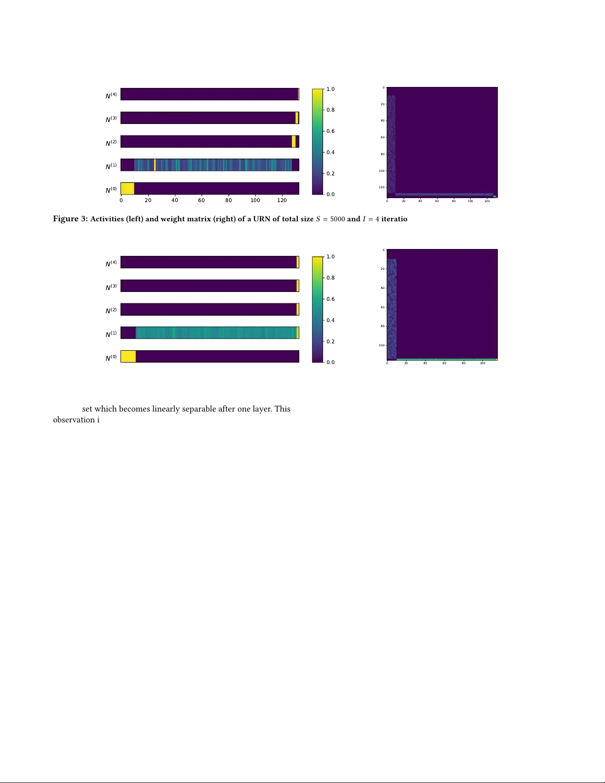
Emergent Structures and Lifetime Structur e Evolution in Artificial Neural Networks Siavash Golkar Flatiron Institute New Y ork University sgolkar@atironinstitute.org ABSTRA CT Motivated by the exibility of biological neural networks whose connectivity structure changes signicantly during their lifetime , we introduce the Unstructured Re cursive Network (URN) and demon- strate that it can exhibit similar exibility during training via gradi- ent descent. W e show empirically that many of the dierent neural network structures commonly used in practice today (including fully connected, locally conne cted and residual networks of dier- ent depths and widths) can emerge dynamically from the same URN. These dierent structures can be derived using gradient descent on a single general loss function where the structure of the data and the relative strengths of various regulator terms determine the structure of the emergent netw ork. W e show that this loss function and the r egulators arise naturally when considering the symmetries of the network as well as the geometric properties of the input data. 1 IN TRODUCTION A remarkable property of biological neural netowrks (BNNs) is their adaptability in the face of ne w environments, dierent tasks and when coping with structure damage [ 1 ]. In contrast, despite their successes, articial neural networks (ANNs) are limited in their applicability , and structures need to be designed for each particu- lar task. Inspired by the genetic evolution of BNNs, an active eld of neural architecture search has emerged leading to spe cialized networks which excel at specic tasks [ 3 ]. However , there is no ANN analog of the lifetime evolution of the structure of BNNs which provide exibility in the face of ne w challenges or damage. The question therefore naturally arises of 1. whether there exist exible ANNs which can adapt their connectivity structure to the task they are trained on during their lifetime and 2. whether ther e exists a new machine learning paradigm based on these exible networks which can compete with the highly specialize d networks in use today . The pr esent work is a small step towar ds answering some of these questions. In particular , we intr oduce the Unstruc- tured Recursive Network (URN), and show that when trained end to end via stochastic gradient descent, a URN dynamically chooses its structure. Specically , dep ending on the geometric structure of the data and the choice of regulator hyperparameters, the same URN can turn into networks which are r ecursive or feedforward, fully connected or lo cally connected (as in CNNs), and can choose whether or not to have residual skip connections. W e also show that the specic form of the URN and the loss function used is mostly determined by various symmetry arguments. Related work Dynamical network architectures where per viously discussed in Fahlman and Lebiere [ 4 ] , where the network is gro wn one neural at a time. Mor e recently , it was shown that r ecurrent neural networks with linear and convolutional lay ers can improv e performance in specic circumstances [ 2 , 7 ]. 2 EMERGEN T STRUCT URES Motivation W e start the discussion by the simple observation that (almost) any network architecture can be embedded in a recursive network. Input Hidden 1 Hidden 2 Output × W 1 × W 2 × W 3 (a) Original network. Input Hidden 1 Hidden 2 Output Input Hidden 1 Hidden 2 Output Input Hidden 1 Hidden 2 Output Input Hidden 1 Hidden 2 Output × W × W × W (b) Equivalent structure. Figure 1: Embedding a multi-layer perceptron (a) in an unrolled unstructured recursive netw ork (b). The purple nodes denote neu- rons that are identically zero. For demonstration, let us consider a feed-for ward neural network with two hidden layers. Fig. 1a shows a cartoon of this network with W i = 1 , 2 , 3 denoting the weights of each layer . W e can emb ed this feed-forward architecture inside a larger recursive structure by concatenating the neurons of all layers as in Fig. 1b and similarly embedding the weights of the dierent layers inside a larger weight matrix W dened as (biases are treated similarly): W = ©    « 0 0 0 0 W 1 0 0 0 0 W 2 0 0 0 0 W 3 0 . ª ® ® ® ¬ (1) It is simple to verify that consecutively applying the W matrix (along with the activation function) 3 times as in Fig. 1b is equivalent to the original MLP network. This block sub-diagonal structure of the weight matrix is a signature of MLPs. In a similar manner , almost all fee d-forward neural networks can b e emb edded in recursive networks. The Unstructured Recursive Network W e now show that it is possible to perform the converse of the above demonstration: starting from a general recursive structure NeurIPS workshop on Real Neurons & Hidden Units, De cemb er 2019, V ancouver , British Columbia, Canada Siavash Golkar without layers, we can arrive at an emergent netw ork which can be interpreted as a feedfor ward multi-layered perceptron. Consider a learning task with d i n and d ou t specifying the dimen- sion of the vectorized input and output. Motivated by the embed- ding arguments of the previous section, we dene a network with as little structure as possible as follows. First, we emb ed the input data in the rst d i n elements of N i , a vector of length S representing all the neurons of the system: N ( 0 ) i = ( x i i ≤ d i n 0 i > d i n , (2) where x i denotes the i ’th component of each vectorized training sample and the superscript ( 0 ) denotes that this is the input of the network (zeroth iteration). W e then dene dene a discreet iterativ e update rule for processing the data: N ( l + 1 ) i = ϕ ( W i j N ( l ) j + b i ) , (3) where W is an S × S matrix, b is the bias, and ϕ is the non-linear activation function. Note that W is initialize d as a (He normal) dense matrix and does not have the block structure of Eq. 1 at the beginning of training. W e apply this update rule a total of I times and then read o the output as the nal d ou t nodes of the neurons. ˆ y i = N ( I ) S − i , i ≤ d ou t (4) A cartoon of this structure is given in Fig. 2 . W e call this architecture the Unstructured Re cursive Network (URN). The only structural hyperparameters here are the total number of neurons S and the number of iterations I . W e will see that neither of these parameters are indicative of the structure of the nal emergent netw ork. Input Output I times N ( 0 ) N ( I ) embed extract Figure 2: Schematic of the Unstructured Recursive Network. W e train this network using standard loss functions and gradient descent methods. Specically , we demonstrate our methodology on classication tasks using a multi-class cross-entropy loss func- tion with added L 1 regulators on b oth network weights as well as the neuron activations after each iteration of the update rule. Correspondingly we have two hyperparameters c W and c N which control the strengths of these regulator terms: L = 1 N Õ L XE ( y , ˆ y ) + c W | W | + c N I Õ l = 1 | N ( l ) | . (5) The use of these regulators is to promote sparsity in the number of active neurons and nonzero weights of the network, which in turn make the emergent structure simpler to interpret. Emergent structures A primary nding of this paper is that when training a URN on a classication task with high values of weight and activity reg- ulation, the top ology of the emergent network is a fe ed-forward multi-layer perceptron. As an example w e train a URN with a total of S = 5000 neurons and I = 4 iterations on a binary classication task comprised of distinguishing inputs sampled from two uniform concentric 10-d spherical shell distributions. Fig. 3 shows a generic result for neural activities and the weight matrix for a network trained on 4000 training samples for 200 epochs with Adam Opti- mizer and learning rate 7 × 10 − 4 , c W = 5 × 10 − 7 and c N = 2 × 10 − 5 (Because of the simplicity of the task in this section, we only choose hyperparameters which consistently lead to 100% test accuracy). For these plots, w e have discarded the inactiv e neurons (i.e. neurons with zero activation) and sorted the remaining neurons according to the iteration number at which they are rst activated. Of the 5000 total initial neurons, only 123 ± 15 (mean + STD across 5 trials) neurons remain active at the end of training. Comparing Fig. 3 to the weight and neural activity structure of the previous section (see Eq. 1 and Fig. 1b ), we see that the neurons have neatly organized into an MLP with 3 hidden layers comprised of 115 ± 15 , 4 ± 1 . 4 , and 3 ± 0 . 7 neurons. In order to ascertain that this structure is indeed the correct topology of the emergent network, we manually set all other weights of the network to zer o and verify there is no change in the network output empirically . For a video of the evolu- tion of a URN during training see https://youtu.be/hvlAnwW - IyY . URN with emergent number of layers In the pre vious section, the number of layers of any emergent MLP is by construction equal to I , the number of the iterations of the recursive network. This is necessarily true since there are I applications of the update rule (Eq. 3 ) in the derivation of the nal values of the output (Eq. 4 ). In order to relax this requirement, we need to allow for pathways in the computation graph of the output values which include dierent numbers of the update rule. The network can then choose dynamically how many ’layers’ to utilize. This can be done using residual connections either on the input or on the output nodes. Residual output no des. Consider the following update rule: N ( l + 1 ) i = ( ϕ ( W i j N ( l ) j + b i ) i < S − d ou t N ( l ) i + ϕ ( W i j N ( l ) j + b i ) i ≥ S − d ou t . (6) This modication has the simple interpretation that it allows for the output of the neural network to accumulate gradually in the output nodes. The network can therefore dynamically cut o further changes to the output after iteration L ≤ I . The number of layers of the emergent network would then eectively b e L . Fig. 4 depicts the results of the training of a URN on the same problem as in the previous section (Fig. 3 ), with the modied update rule in Eq. 6 . The emergent network now has one hidden layer (compared to three in the previous section) despite the number of iterations I being 4. This can be attributed to the ( lack of ) complexity of Emergent Structures and Lifetime Structure Evolution in Artificial Neural Networks NeurIPS workshop on Real Neurons & Hidden Units, De cemb er 2019, V ancouver , British Columbia, Canada N ( 4 ) N ( 3 ) N ( 2 ) N ( 1 ) 0 20 40 60 80 100 120 N ( 0 ) 0.0 0.2 0.4 0.6 0.8 1.0 0 20 40 60 80 100 120 0 20 40 60 80 100 120 Figure 3: Activities (left) and weight matrix (right) of a URN of total size S = 5000 and I = 4 iterations on the concentric sphere dataset with d = 10 . The weight matrix and activities of neurons exhibit an emergent MLP structure. N ( 4 ) N ( 3 ) N ( 2 ) N ( 1 ) N ( 0 ) 0.0 0.2 0.4 0.6 0.8 1.0 0 20 40 60 80 100 0 20 40 60 80 100 Figure 4: Same setting as Fig. 3 with output nodes which have a residual update rule (Eq. 6 ). the dataset which becomes linearly separable after one layer . This observation is further reinforced in Sec. 3 where in a more dicult problem ( classication on CIF AR-10) the emergent network utilizes the maximum allowed number of layers (i.e. L = I ). Residual input nodes. This alternative modication has the intu- itive interpr etation of continuously feeding the input into the input nodes at every step of the iteration: N ( l + 1 ) i = ( x i + ϕ ( W i j N ( l ) j + b i ) i ≤ d i n ϕ ( W i j N ( l ) j + b i ) i > d i n . (7) The implementation of residual connections on the input nodes has the advantage that it allows for the formation of skip connections in the emergent network. How ever , because of this mixing of dierent layers (i.e. neurons that have dier ent numbers of iterations of the update rule applied), it also leads to neural activity patterns that ar e harder to interpret in terms of a simple feed-for ward network. W e leave the analysis of the emergence of more complicated networks with skip connections and feedback lo ops to future work. 3 INCORPORA TING INP U T STRUCT URE In this section we discuss the circumstances under which convo- lutional NNs (CNN) or rather locally connected networks (LCN) which are CNNs without weight sharing can arise from a URN. In an LCN, the neurons of each layer are connected to a small neigh- borhood of neurons in the previous layer . The denition of this neighborhood implicitly requires a proximity or a distance mea- sure dened on the neurons or on the individual comp onents of the input. Consequently , a dataset which has no such proximity information, or more generally datasets which are invariant under permutation of the components of the input (such as the spheres in Sec. 2 ), combined with an update rule which preser ves this symme- try (e.g. Eq. 3 ), would generally lead to emergent structures which also respect this permutation symmetr y and hence do not have lo- cal connectivity structure. This permutation symmetr y is naturally broken in many tasks. Here, we specialize to image recognition as an example and show how this symmetry breaking naturally leads to emergent networks with local connectivity structure. Let us assume that the input of the network is a two-dimensional matrix of size d x × d y . Implicit in this notation is the assumption of a Euclidean metric which determines the relative distance of dierent pixels on the 2D plane (the argument also applies to cur ved or other non-trivial geometries). It is therefore natural that when we embed this metric space inside the larger structure of the URN, there will be also be a metric induce d on this larger space given by the uplift of the 2D Euclidean metric of the input. The simplest such metric would be a product metric where there is a single extra dimension perpendicular to the nodes assigne d as the input (see Fig. 5 ): d s 2 = d s 2 input + β d z 2 , (8) where β is a hyperparameter determining the perpendicular length scale compared to the directions parallel to the input. This induced geometric structure on the neur ons of the network allows us to add extra regulator terms to the loss function which ar e interpretable as p enalizing the synaptic length connecting dierent NeurIPS workshop on Real Neurons & Hidden Units, De cemb er 2019, V ancouver , British Columbia, Canada Siavash Golkar Embed x y x y z Figure 5: Emb edding an input with geometric structure in the neu- rons of the URN. A metric on the input samples ( left) naturally in- duces a metric structure on this larger space (right). neurons. Thi s term was not allow ed under the permutation symme- try of the previous section. Also, this term is still invariant under the parts of the permutation symmetry which remain unbroken after the addition of the metric structure (e.g. discrete 90 degree rotations). L = 1 N Õ L XE ( y , ˆ y ) + c W | W | + c N I Õ l = 1 | N ( l ) | + c syn Õ i < j | W i j | d γ i j , (9) where c W and c N are as before, d i j is the distance of the i ’th and j ’th neuron under the metric in Eq. 8 , γ is the distance power hyper- parameter , and c len determines the strength of the ne w regulator term penalizing the length of each synapse. W e performed an experiment using monochromatic CIF AR-10 images using a URN with an uplift ge ometry e quivalent to a x × y × z cube of 60 × 60 × 6 = 21 , 600 total neurons (see Fig. 5 ). The input embedding rule (Eq. 2 ) is modied as follo ws: the 32 × 32 inputs are expanded to 60 × 60 using interp olation and are embedded in the z = 1 neurons. W e use I = 4 iterations of the residual output update rule describe d in Eq. 6 . Finally , the center 10 neurons at z = 6 or designated as the output nodes. The emergent network structure is depicted in Fig. 6 , where for ward going weights (connecting smaller z neurons to larger z neurons) are depicted in red, backward going weights in green and equal z weights are depicted in black. A clear feedfor ward and lo cally connecte d structure is appar ent with a very few green/black weights. Without hyperparameter ne-tuning this network achieves a test accuracy of 52%, a 10% impro vement over the same structure with only weight and activity regulators. Figure 6: Conne ctomics of a URN trained on CIF AR-10 with synap- tic length regularization. 4 DISCUSSION In this paper we have an empirical demonstration that many of the neural network structures in use to day can dynamically emerge from the same general framework of the URN. W e showed in exam- ples that the nal topology of these networks is easily interpr etable as feed-forward MLPs with number of layers and number of neu- rons per layer determine d during training. Furthermore, we showed that given input data with proximity information ( e.g. a metric), we can naturally extend the URN loss function such that we can derive locally connected networks whose generalization performance is considerably improved. These demonstrations, ho wever , are only the rst stages of this project and much work r emains to be done. For example, one can ask, how does the emergent netw ork topology vary with task diculty . This question is currently under study and beyond the scope of the demonstrations in this paper . One can also ask many other questions: e.g. under what circumstances, if any , recurrent neural NNs emerge from a URN or if it is p ossible to somehow naturally incorporate weight sharing such that we can arrive at a convolutional network. Finally , a the oretical understand- ing of why we generically arrive at fee d-forward networks beyond simple intuitive arguments is still needed. Never-Ending Structure Accumulation. In light of the recent works in continual and never-ending learning [ 6 ], and to circle back to the points raised in the introduction, we propose the follow- ing alternative learning scheme. Let us assume that we are given a series of related tasks of gradually increasing diculty . For example, in vision, these can start from simple edge detection and end with image classication. W e can intuitively predict what will happen if we train a network with dynamically chosen architecture on these tasks consecutively using a compatible lifelong learning algorithm which minimizes performance loss on prior tasks. When trained on the simple tasks, the emergent network would be shallow with few layers. However , as more complex tasks ar e trained, the depth of the network would gr ow and each consecutive tasks would naturally build on top of the structures already present in the architecture. Preliminary results show that this expectation is borne out when training a URN in conjunction with the lifelong learning algorithm from Golkar et al. [ 5 ] on a series of simple to dicult image tasks. This line of argument and experiments suggest an alternative learning paradigm to today’s highly specialized networks speci- cally built for each task. In this learning paradigm, which w e dub Never-Ending Structure Accumulation or NESA, the structure is simply determined by the series of simple to dicult tasks which culminate in the nal ML problem of interest. The responsibility of the ML practitioner in NESA would then b e to design this series tasks. While this is not a trivial undertaking for many ML problems, it brings the problem of training ANNs much closer to how BNNs learn to perform new tasks during their lifetime. Acknowledgments. W e would like to thank Jack Hidar y , K yunghyun Cho, Cristina Savin, Owen Marschall, Y ann LeCun, Dmitri Chklovskii and Anirvan Sengupta for interesting discussions and input. This work is partly supported by the James Arthur Postdoctoral Fellow- ship. Emergent Structures and Lifetime Structure Evolution in Artificial Neural Networks NeurIPS workshop on Real Neurons & Hidden Units, De cemb er 2019, V ancouver , British Columbia, Canada REFERENCES [1] D. B. Chklovskii, B. W . Mel, and K. Svoboda. 2004. Cortical rewiring and informa- tion storage. Nature 431, 7010 (2004), 782–788. https://doi.org/10.1038/nature03012 [2] David Eigen, Jason Rolfe, Rob Fergus, and Y ann LeCun. 2013. Understanding Deep Architectures using a Recursive Convolutional Network. arXiv e-prints , Article arXiv:1312.1847 (Dec 2013), arXiv:1312.1847 pages. arXiv: cs.LG/1312.1847 [3] Thomas Elsken, Jan Hendrik Metzen, and Frank Hutter. 2018. Neural Architecture Search: A Survey. , Article arXiv:1808.05377 (Aug. 2018), arXiv:1808.05377 pages. arXiv: stat.ML/1808.05377 [4] Scott E. Fahlman and Christian Lebiere. 1990. Advances in Neural Information Processing Systems 2. Chapter The Cascade-correlation Learning Architecture, 524–532. http://dl.acm.org/citation.cfm?id=109230.107380 [5] Siavash Golkar, Michael Kagan, and K yunghyun Cho. 2019. Continual Learning via Neural Pruning. (Mar 2019). arXiv: cs.LG/1903.04476 [6] T . Mitchell, W . Cohen, E. Hruschka, P. T alukdar , B. Y ang, J. Betteridge, A. Carlson, B. Dalvi, M. Gardner , B. Kisiel, J. Krishnamurthy , N. Lao, K. Mazaitis, T . Mohamed, N. Nakashole, E. Platanios, A. Ritter , M. Samadi, B. Settles, R. W ang, D. Wijaya, A. Gupta, X. Chen, A. Saparov , M. Greaves, and J. W elling. 2018. Never-ending Learning. Commun. ACM 61, 5 (April 2018), 103–115. https://doi.org/10.1145/ 3191513 [7] Jason T yler Rolfe and Y ann LeCun. 2013. Discriminative Recurrent Sparse A uto- Encoders. arXiv e-prints , Article arXiv:1301.3775 (Jan 2013), arXiv:1301.3775 pages. arXiv: cs.LG/1301.3775