Ground Truth Simulation for Deep Learning Classification of Mid-Resolution Venus Images Via Unmixing of High-Resolution Hyperspectral Fenix Data

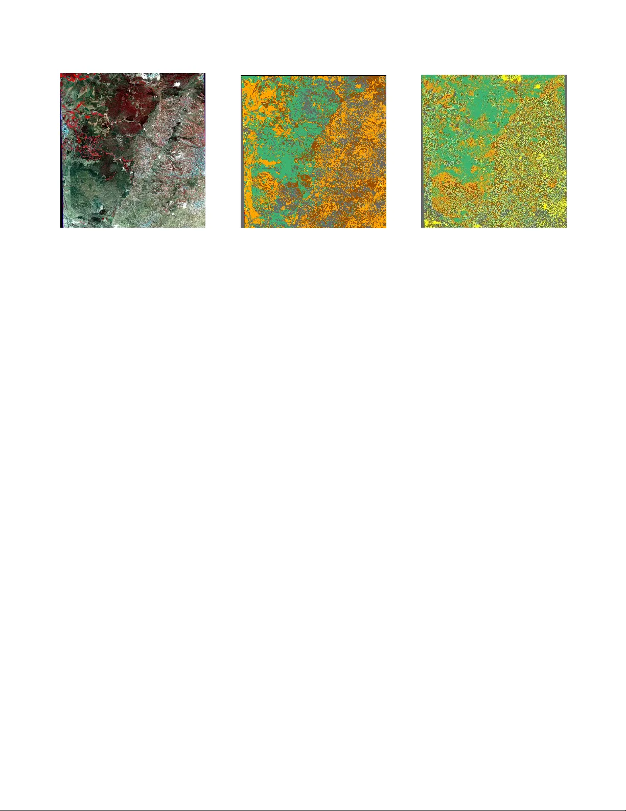
GR OUND TR UTH SIMULA TION FOR DEEP LEARNING CLASSIFICA TION OF MID-RESOLUTION VENUS IMA GES VIA UNMIXING OF HIGH-RESOLUTION HYPERSPECTRAL FENIX D A T A Ido F aran, Nathan S. Netanyahu Eli (Omid) David Bar-Ilan Uni versity Dept. of Computer Science ramat-gan 5290002, Israel Maxim Shoshany , F adi Kizel Jisung Geba Chang, Ronit Rud T echnion Israel Institute of T echnology Faculty of Ci vil and En vironmental Engineering Haifa 3200003, Israel ABSTRA CT T raining a deep neural network for classification constitutes a major problem in remote sensing due to the lack of adequate field data. Acquiring high-resolution ground truth (GT) by human interpretation is both cost-ineffecti ve and inconsistent. W e propose, instead, to utilize high-resolution, h yperspectral images for solving this problem, by unmixing these images to obtain reliable GT for training a deep network. Specifically , we simulate GT from high-resolution, hyperspectral FENIX images, and use it for training a con volutional neural network (CNN) for pixel-based classification. W e show ho w the model can be transferred successfully to classify ne w mid-resolution VEN µ S imagery . Index T erms — VEN µ S satellite, hyperspectral image classification, unmixing, deep learning, con volutional neural network. 1 Intr oduction Pixel-based classification of hyperspectral images is a major task in remote sensing, which inv olves assigning a class la- bel to ev ery pixel of an input image. This task, also known as pixel-wise classification or semantic segmentation, has at- tracted man y studies over the years. V arious methods hav e been proposed for this task. The traditional approach classi- fies hand-crafted features, using support vector machines [1], morphological profiles [2], sparse representation [3], etc. Howe ver , these methods rely typically on human exper - tise for tuning them on a specific dataset and they can extract only “shallo w” features of the original data [4]. An alternative approach is to extract useful features directly from the image pixels. Deep learning (DL) models ha ve prov en to be suitable for this kind of problem [5]. Such models are trained on image data sets, and are capable of learning both low-le vel and high- lev el feature representations directly from an input image, due to their deep hierarchical architectures. In addition, some DL models can exploit both spectral and spatial features of hyper- spectral images, leading to improv ed classification results. DL models can be categorized to supervised and unsu- pervised models. Unsupervised models (e.g., auto-encoders), are trained to extract features from large unlabeled data sets. By restricting the encoder-decoder structure, one can adjust the model to achiev e the results of the required task [6] [7] [8]. Supervised models (e.g., convolutional neur al networks (CNNs) and deep belief networks) are trained using ground truth (GT) information as e xpected output of the netw ork. In principle, supervised networks can learn more precise fea- tures by exploiting the label-specific information from the training data [9] [10] [11]. Although most supervised models achiev e superior classi- fication, they rely on a considerable amount of GT for training the model. Additionally , there is a limited amount of labeled datasets in the remote sensing community [5], especially for a new source of information such as a ne w satellite. The V e getation and En vir onment monitoring New Micr o- Satellite (VEN µ S) is a ne w satellite that w as launched in Au- gust 2017. It acquires frequent, high-resolution multispectral images of o ver 100 sites of interest around the world. This enables monitoring of plant growth and their health status, as well as the impact of en vironmental factors, such as hu- man acti vities and climate change, on land surfaces of the Earth [12]. Up to this day , there is a relativ ely small number of images acquired by VEN µ S and virtually no GT for training a model on this data. Thus, in an attempt to ov ercome the lack of labeled VEN µ S data, and in order to start using these images in supervised models, we need to generate GT correlated with the satellite data acquired. T o av oid the expensiv e task of obtaining a large number of labeled samples, we propose a nov el method for simulating GT from a higher spectral resolution airborne sensor , and us- ing it as initial training data for a CNN model. By applying a state-of-the-art spectral unmixing algorithm [13] to the abov e airborne data, and adapting the acquired images to the spa- tial and spectral resolutions of VEN µ S, we can train a CNN Ref: IEEE International Geoscience and Remote Sensing Symposium (IGARSS) , pages 807–810, Y okohama, Japan, July 2019. Fig. 1 : FENIX flight strip ov er Israel to classify VEN µ S images to se veral predefined endmembers (EMs). This approach may help provide initial classification of incoming VEN µ S images, without any GT , as part of a more comprehensi ve ef fort of processing time-series VEN µ S data on a continuous basis. The paper’ s contributions are as follows: (1) Introduction of a novel GT simulation for training a DL-classification model without manual labeling, (2) presentation for the first time of classification results for the recently launched VEN µ S satellite ov er a Mediterranean region that is of much interest (as far as climate change is concerned), i.e., the re- sults can serve as a baseline for comparison with further methods, and (3) providing simulated data that will allow us to train more sophisticated models (such as fully con volu- tional neural network [14]) or explore more complex tasks, such as spectral unmixing using neural networks, for further processing of VEN µ S data. 2 Backgr ound 2.1 FENIX A FENIX airborne scan took place on April 04, 2017 under clear sky conditions, along a transect from the Beit-Guvrin area (representing a semi-arid region with a rainfall rate of 450[mm/year]) to Leha vim (representing a desert fringe zone with 250[mm/year] rainfall). The scan was carried out over a 35-[km] long strip with a swath of 1.5[km] (Figure 1). A SPECIM AisaFENIX 1K airborne system was mounted on a Cessna 172 airplane flying at an altitude of 1,828[m] abov e sea le vel over a topographic area with an average height of 250[m]. The system consisted of VNIR and SWIR instruments, yielding a ground sampling distance of 1[m], and having wa velength ranges of 380-970[nm] (at 4.5[nm] spectral resolution) and 970-2500[nm] (at 12[nm] spectral resolution), respectively . The spectral bands were resampled into 41 bands of 5[nm] width in the wav elength range of 400-2400[nm]. 2.2 VEN µ S The VEN µ S satellite carries a super-spectral camera charac- terized by 12 narro w spectral bands ranging from 415[nm] to 910[nm]. The radiometric resolution for all bands is 10 bits and the spatial resolution is 5[m]. The spectral resolu- tion at the V is-NIR range is 40[nm], and 16[nm] and 20[nm], respectiv ely , for the red edge and water vapor bands. Each experimental site is of size 27 × 27 [km], with a 2-day revisit time. 2.3 Spectral Unmixing Giv en a spectral image and the spectra of a set of distinct EM materials, the spectral unmixing process allows for extract- ing quantitativ e subpixel information by estimating the abun- dance fraction of each EM, in each pixel. Assuming a linear mixtur e model (LMM), we write the spectral signature of each pixel as follo ws: m = Ef + n where m = [ m 1 , ..., m λ ] T is a signature of mixed pixel, λ is the number of spectral bands, E ∈ R λ × d is the matrix of d EMs, f ∈ R d × 1 is a vector of the corresponding fractions, and n ∈ R λ × 1 represents the system noise and assumed to be Gaussian with zero mean. Requiring a fully constrained solution, the unmixing problem is solved subject to two con- straints: f i ≥ 0 for i = 1 , . . . , d , and f T 1 ≤ 1 , where 1 ∈ R d × 1 is a vector of ones. In our case, we use the vec- torized code projected gradient descent unmixing (VPGDU) method [13]. VPGDU combines the pr ojected gr adient de- scent (PGD) and an exact line search strategy to optimize an objective function that is based on spectral angle mapper (SAM). 2.4 Con volutional Neural Network (CNN) CNNs hav e shown excellent performance in various visual perception tasks, such as object detection, object classifica- tion, semantic segmentation, etc., by exploiting the local con- nectivity between adjacent pixels. Recently , CNNs hav e also been used successfully for classification of hyperspectral im- ages; see, e.g., Hu et al. [9], Makantasis at el. [10], and Y ue et al. [11]. 3 PR OPOSED METHOD 3.1 Overview Figure 2 illustrates the framew ork of the proposed method. It consists of three parts: (1) Ground truth simulation, (2) train- ing a CNN model, and (3) e valuating its classification on a real VEN µ S image. In the first part, a spectral unmixing al- gorithm is executed on higher -resolution images using pre- defined labels and their estimated abundance vectors in order to extract fraction vectors. The original images are then ag- gregated and adjusted to match VEN µ S’ s spatial and spectral resolutions. In the second step, we use spatial patches around each labeled pixel to train a deep CNN. Finally , we apply the trained network to a calibrated VEN µ S L1 image to obt ain its classification map. The proposed method is described below in detail. Fig. 2 : Architecture of proposed method: CNN trained using simulated GT from hyperspectral image, and then used for classification of mid-resolution image. Fig. 3 : Illustration of synthesized GT pixel labels based on unmixing results. 3.2 Ground T ruth Simulation W e simulate plausible GT for VEN µ S by conv erting a giv en FENIX image (at 1[m] resolution). Non-contiguous regions of 5 × 5 pixels are aggregated to a single pixel (at 5[m] res- olution), and only the bands matching VEN µ S’ s spectral res- olution are selected. T o synthesize the GT labels (Figure 3), we first generate fraction maps of the high-resolution FENIX image (by applying VPGDU with respect to the se ven EMs selected). The label assigned to a gi ven pixel of the simulated VEN µ S image is the EM for which the aggregated fractions (ov er the corresponding 5 × 5 region in the FENIX image) is the greatest. 3.3 T raining Neural Networks The simulated input images are split to small patches [15] [16]. Each patch contains a spatially correlated area around a specific pixel and its label as explained above. This allows for creating a large amount of label samples for training. W e examined several DL models for the classification task; the best results were achiev ed for a deep CNN model. The proposed network receives an n × m × b input matrix (where n , m are the patch dimensions, and b is the number of spectral bands). It consists of L con volution layers with a decreasing amount of filters per layer . Because of the rela- tiv ely small input size, max-pooling layers are not necessary to simplify the dimensions of the model. Finally , the output of the last conv olution layer is flattened and fed into a number of fully connected layers. The softmax activ ation function is applied to the last layer’ s output for creating classification fractions. The output label of the center pixel of the patch is determined by the class of the greatest fraction. In addition, due to the unbalanced amount of samples per label, data augmentation and denoising layers are added to prev ent the network from over -fitting to the most frequent la- bels. Adding Gaussian noise, random rotations and image mirroring are used for creating balanced label counts per sam- ple. Batch normalization [17] and dropout [18] layers are also added between hidden layers to insert noise into the training process. 3.4 Evaluating on New Dataset The classification due to the trained network can be “trans- ferred” to new images acquired over similar geographical re- gions with the same EMs. This is applied to VEN µ S images at the L1 lev el (that were geographically calibrated to clean background noises while preserving spatial resolution). Im- age patches (from the real VEN µ S image) are then fed into the trained network as before to obtain a classification label for their center pixels. 4 EXPERIMENT AL RESUL TS 4.1 Datasets The suggested procedure has been tested on simulated and real VEN µ S images for quantitati ve/visual assessment. The simulated training data was acquired from the FENIX dataset by taking the the six most relev ant areas, with an av- erage picture size of 400 × 100 pixels. The VEN µ S test data of size 6829 × 7824 pixels, with a spatial resolution of 5[m] and 11 spectral bands 1 , was ac- quired ov er the S02 polygon of Israel [19] on June 15, 2018. W e worked with atmospherically corrected L1 products to maintain the original spatial resolution. The following se ven EMs that match the common land composition in this area were selected: Brown Soil, Light Soil, Rock, T all Tree/Shrub, Dwarf Shrub, Herbaceous, and Dense Shrub/Burned Area. 4.2 Parameters and Details T o obtain reliable results, we conducted a 6-fold cross v alida- tion; each time one of the images was left out for testing, and the rest were used for training and v alidation. Specifically , all of the pix els of the latter images were randomly shuf fled, and each time 90% of these pixels were used for training and the remaining 10% of the pixels for validation. Also, we normal- ized the images, as part of preprocessing, by standardizing the 1 band 6 is removed, as it is a duplication of band 5 for image quality (a) False color composite (b) Ground T ruth (c) CNN classification Fig. 4 : V isualization of the results obtained ov er the A visure2 area. values of each spectral band to have zero mean and a standard deviation of 1.0. After examining sev eral patch configurations, we selected 5 × 5 patches (i.e., 25[ m ] × 25[ m ] regions) around each pixel, labeled according to the center pix el of the patch. T o train a balanced model with a similar count of samples per label, data augmentation was applied via horizontal/vertical flips, rotations by 90 ◦ , 180 ◦ , and 270 ◦ , and addition of Gaussian noise with zero mean and 0.1 standard de viation. During each epoch, 30,000 samples per label (for a total of 210,000 sam- ples in each epoch) were created using a combination of the abov e techniques. The full network architecture is shown in Figure 2. For the CNN model, we used 4 layers of 3 × 3 con volution filters, with a different amount of filters per layer , i.e., 64, 64, 32, and 16 filters, respectiv ely . Batch normalization layers are used (before applying a ReLU acti v ation function), as well as dropout layers with a rate of 25%. The CNN is follo wed by 3 fully connected layers with an output size of 7 neurons. (The hidden layers are activ ated using the ReLU function, while the output layer uses softmax activ ation.) The following hyperparameters were arrived at after var - ious tuning attempts: Batch size = 64, cross entropy loss function, and Adam optimizer with a learning rate of 0.001. All weights were randomly initialized. The deep neural net- work was implemented using the Python programming lan- guage with T ensorFlow as the DL framew ork. The network was trained ov er 200 epochs using backpropagation on a PC equipped with Intel Core I7 and Nvidia GeForce GTX 1080 T i GPU. T esting Image V alidation Accuracy T est Accurac y Amazya1 80.67% 69.40% A visure1 82.65% 69.97% A visure2 80.61% 75.08% Between1 80.48% 70.96% Between2 82.49% 73.27% Lehavim1 80.80% 76.71% Overall 81.29% 72.56% T able 1 : Classification results on FENIX test images. 4.3 Results T able 1 reports the classification results obtains by the pro- posed network on the 6 test images. The a verage accuracy obtained was ∼ 72 . 6% . Although the quantitativ e results are not extremely high, visual assessment rev eals a notable simi- larity between GT and the classification maps for large parts of the simulated and real VEN µ S images (Figures 4 and 5, respectiv ely). This should attest to the good promise of our baseline method for further classification of ne w VEN µ S im- ages. 5 CONCLUSION W e proposed a novel method for GT simulation of mid- resolution data by applying unmixing to high-resolution hy- perspectral images. This allows to overcome a fundamental problem in remote sensing, i.e., a severe lack of labeled data. The simulated data was used for initial training of a CNN for pixel-based classification, as part of an ongoing project of temporally evolving CNNs for the analysis of the ecolog- ical mapping of Mediterranean en vironments using VEN µ S images. 6 Refer ences [1] F . Melgani and L. Bruzzone, “Classification of hyper- spectral remote sensing images with support vector ma- chines, ” IEEE T rans. Geosci. Remote Sens. , vol. 42, no. 8, pp. 1778–1790, 2004. [2] M. Fauvel, J. A. Benediktsson, J. Chanussot, and J. R. Sveinsson, “Spectral and spatial classification of hyper- spectral data using SVMs and morphological profiles, ” IEEE T rans. Geoscience and Remote Sensing , vol. 46, no. 11, pp. 3804–3814, 2008. [3] Y . Chen, N. M. Nasrabadi, and T . D. T ran, “Hyperspec- tral image classification using dictionary-based sparse representation, ” IEEE T rans. Geosci. Remote Sens. , v ol. 49, no. 10, pp. 3973–3985, 2011. [4] J. M. Bioucas-Dias, A. Plaza, G. Camps-V alls, P . Sche- unders, N. Nasrabadi, and J. Chanussot, “Hyperspec- tral remote sensing data analysis and future challenges, ” (a) False color composite (b) CNN classification (c) ISOD A T A output Fig. 5 : V isualization of the results on a real VEN µ S image. IEEE Geosci. Remote Sens. Mag. , vol. 1, no. 2, pp. 6– 36, 2013. [5] L. Zhang, L. Zhang, and B. Du, “Deep learning for remote sensing data: A technical tutorial on the state of the art, ” IEEE Geosci. Remote Sens. Mag. , v ol. 4, no. 2, pp. 22–40, 2016. [6] R. K emker and C. Kanan, “Self-taught feature learn- ing for hyperspectral image classification, ” IEEE T rans. Geosci. Remote Sens. , vol. 55, no. 5, pp. 2693–2705, 2017. [7] Z. Lin, Y . Chen, X. Zhao, and G. W ang, “Spectral- spatial classification of hyperspectral image using au- toencoders, ” in 9th IEEE Int. Conf. Inf., Commun. & Signal Pr ocess. IEEE, 2013, pp. 1–5. [8] C. T ao, H. Pan, Y . Li, and Z. Zou, “Unsupervised spectral–spatial feature learning with stacked sparse autoencoder for hyperspectral imagery classification, ” IEEE Geosci. Remote Sens. Lett. , vol. 12, no. 12, pp. 2438–2442, 2015. [9] W . Hu, Y . Huang, L. W ei, F . Zhang, and H. Li, “Deep con volutional neural networks for hyperspectral image classification, ” J . Sensors , v ol. 2015, 2015. [10] K. Makantasis, K. Karantzalos, A. Doulamis, and N. Doulamis, “Deep supervised learning for hyperspec- tral data classification through con volutional neural net- works, ” in IEEE Int. Symp. Geosci. Remote Sens. IEEE, 2015, pp. 4959–4962. [11] J. Y ue, W . Zhao, S. Mao, and H. Liu, “Spectral–spatial classification of hyperspectral images using deep con vo- lutional neural networks, ” Remote Sens. Lett. , v ol. 6, no. 6, pp. 468–477, 2015. [12] “V enus W ebsite, ” https://venus.cnes.fr/en/ VENUS/index.htm . [13] F . Kizel, M. Shoshany , N. S. Netanyahu, G. Even-Tzur , and J. A. Benediktsson, “ A stepwise analytical projected gradient descent search for hyperspectral unmixing and its code vectorization, ” IEEE T rans. Geosci. Remote Sens. , vol. 55, no. 9, pp. 4925–4943, 2017. [14] J. Long, E. Shelhamer , and T . Darrell, “Fully con volu- tional networks for semantic segmentation, ” in IEEE Conf. Comput. V is. P attern Recog . , 2015, pp. 3431– 3440. [15] J. Y ang, Y .-Q. Zhao, and J. C.-W . Chan, “Learning and transferring deep joint spectral–spatial features for hy- perspectral classification, ” IEEE T rans. Geosci. Remote Sens. , vol. 55, no. 8, pp. 4729–4742, 2017. [16] Y . Chen, Z. Lin, X. Zhao, G. W ang, and Y . Gu, “Deep learning-based classification of hyperspectral data, ” IEEE J. Sel. T opics Appl. Earth Obs. Remote Sens. , vol. 7, no. 6, pp. 2094–2107, 2014. [17] S. Iof fe and C. Szegedy , “Batch normalization: Acceler- ating deep netw ork training by reducing internal cov ari- ate shift, ” arXiv preprint , 2015. [18] N. Sriv astav a, G. Hinton, A. Krizhevsk y , I. Sutske ver , and R. Salakhutdinov , “Dropout: A simple way to pre- vent neural networks from ov erfitting, ” J. Mach. Learn. Res. , vol. 15, no. 1, pp. 1929–1958, 2014. [19] “V enus Israel W ebsite, ” https://venus.bgu.ac. il/venus .