DCSO: Dynamic Combination of Detector Scores for Outlier Ensembles

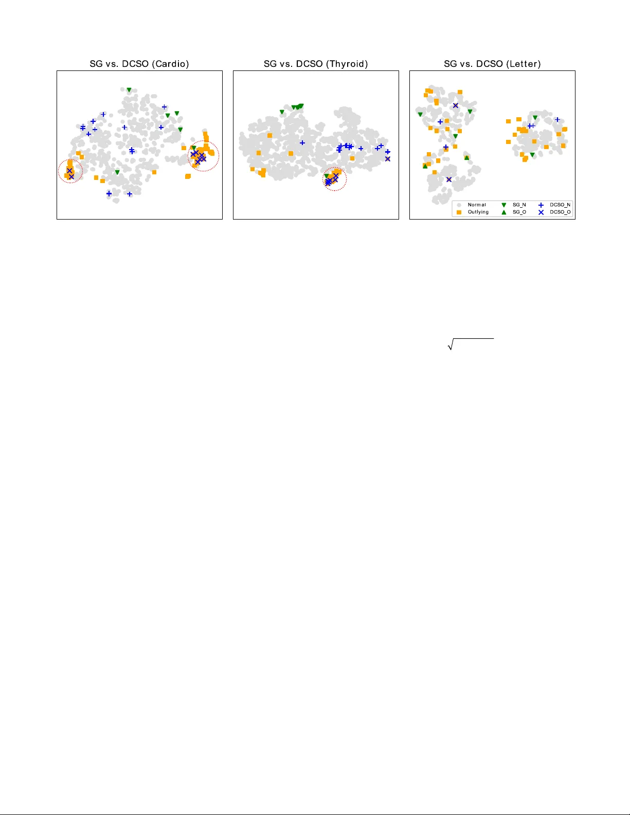
Outlier Ensembles Yue Zhao Department of Computer Science University of Toronto Toronto, Canada yuezhao@cs.toronto.edu Maciej K. Hryniewicki Data Assurance & A nalytics PricewaterhouseCoopers Toronto, Canada maciej.k.hryni ewicki@pwc.com ABSTRACT Selecting and combining the outlier scores of different base detectors used within outlier ens embles can be quite challengin g in the absence of ground truth. In this paper, an unsupervised outlier detector combination framework called DCSO is proposed, demonstrated and assessed for th e dynamic selection of most competent base detectors, with an emphasis on data locality. Th e proposed DCSO framework first defines the local region of a tes t instance by its k nearest neighbors and then identifies the top- performing base detectors within t he local region. Experimental results on ten ben chmark datasets d emonstrate that DCSO provides consistent performance i mprovement over existing stati c combination approaches in mining outlying objects. To facilitat e interpretability and reliability of the proposed method, DCSO i s analyzed using both theoret ica l frameworks and visualization techniques, and presented alongside empirical param eter setting instructions that can b e used to improve the over all performanc e. Keywords Outlier ensembles, outlier detection, anomaly detection, ensemb le learning, model com bination, dynamic c lassifier selection 1. INTRODUCTION Outlier detection methods aim to identify anomalous data points from normal ones and are useful in many applications including the detection of anomalous behavior in social media [10] as wel l as the detection of faulty mechanical devices [9]. Over the yea rs, numerous unsupervised outlier d etection methods have been proposed [7, 21–23] because the ground truth is often absent in outlier mining [1]. In spite of some recent successes in outlie r detection, unsupervised approaches have been critici zed for yielding both high false positive and high false neg ative rat es [12]. To improve the detection accuracy and stability, research ers have recently devoted their effo rts to the application of ensem ble methods to outlier detection problems [1, 2, 31, 38], and sever al new outlier ensemble algorithms h ave been proposed [22, 23, 30, 31, 37]. Ensemble learning uses combinations of various base estimators to achieve more reliab le and superior results than t hose attainable with an individual e stimator [14, 19]. This appro ach typically involves two key stag es [31]: (i) the Generation stage, which creates a pool of base estimators and (ii) the Combination stage , which synthetizes the base estimators to create an improved final output. The model combina tion is particularly important, as there is often an inherent risk that some of the constituent estimators could potentiall y deteriorate the capabilities of th e ensemble, rather than improve them [29, 30]. Although existing outlier ensemble methods show promising results, there is still room for improvement as the mode l combination stage could be quite challengi ng at times [1] . First of all, most existing combination methods are fully stati c and do not involve any detector sel ection processes, even though th ey are critical in detector combina tion for outlier ensembles [30] . The lack of detector selection limits the benefits of model combina tion as base detectors may not be fully capable of identifying all o f the unknown outlier instances [11]. Although static averaging of al l base detector scores is the most widely used method, it could possibly have the high-performi ng detectors being neutralized b y the low-performing ones in ove rall model perform ance [2]. Secondly, the importance of dat a locality is oft en underestimat ed and rarely discussed in detecto r selection and combination. Specifically, the competency of a base detector is typically evaluated globally on all training data points instead of being on the local region related to the test object. For instance, a po pular combination method called weighted averaging [38] uses the Pearson correlation between the detector score and the pseudo ground truth on a ll training points as the detector weight [38] . Numerous local detection algorithms [7, 21, 33] have therefore been developed as of late, under the premise that certain types o f outliers are more easily identified by local data relationships [33]. As a result, considering the base detector performance in the l ocal region of a test instance may be helpful to detector selection and combination. Thirdly, limited interpretability and reliability of unsupervis ed combination frameworks prevent these methods from being used in mission-critic al tasks. Some possible causes include: (i) th e lack of ground truth impedes a controlled combination process; (ii) the c ombination framework s may involve random processes leading to unstable performance and poor reproducibility; (iii) only the combination result is available, but the decision procedure is untraceable and (iv) algorithm results are often analyzed b y direct com parison instead of s tatistical analysis. To address the aforementioned limitations, a fully unsupervised framework called DCSO ( D ynamic C ombination of Detector S cores for O utlier Ensembles) is pr oposed in this research to select and combine base detectors dynamically with a focus on data localit y. The idea is motiva ted by an established supervis ed ensemble framework known as Dynamic Classifier Selection (DCS) [19]. DCS selects the best classifier for each test insta nce Permission to m ake digital or hard copies of all or part of thi s work for personal or classroom use is granted without fee provided that copies are not made or d istributed for profit or commercial advantage and that copies bear this notice and the full citation on the first page. To co py otherwise, or republish, to post on servers or to redistribute to lists, r equires prior specific permission and/or a fee. ACM SIGKDD Workshop on Outlier Detection De-constructed (ODD v5.0 ), August 20, 2018, London, UK. ACM ISBN 123-4567-24-5 67/08/06…$15.00 https://doi.org/10.475/123_4 © 2018 Copyright held by the owner/author(s). DCSO: Dynamic Combination of Detector Scores for on the fly by evaluating base cla ssifiers’ competency on the lo cal region of a test instance [11]. The rationale behind this is th at not every base classifier is good a t categorizing all unknown test instances and may be more like ly to specialize in different loc al regions [11]. Similarly, DCSO fi rst defines the local region of a test instance as its k nearest training points, and then identifies the most competent base detector in the local region by t he similar ity to the pseudo ground truth. To further improve algorithm stabil ity and capacity, ensem ble variations of DCSO are proposed: multiple promising detectors are kept for a second-phase combination instead of only using the most c ompetent detector. To the best of the authors’ knowledge, this is the first publis hed effort to adapt DCS from supervised classification tasks to unsupervised outlier ensembles. The proposed DCSO framework has th e following advantag es: 1. DCSO outperforms traditiona l static methods on most datasets with a significant i mprovement in precision; 2. DCSO has great extensibility as it is compatible with different types of base detectors, such as Local Outlier Factor (LOF) [7] and k Nearest Neighbors ( k NN); 3. DCSO can show the combination process for each test instance by providing the selected base detector(s), which helps model valida tion and reproducibility. To improve model interpretability and deconstruct the black-box nature of outlier detector combi nation, various a nalysis method s are employed herein. First, a theoretical explanation is provid ed under a recently proposed framework by Aggarwal and Sathe [3]. Second, visualization techniques are lever aged to intuitively explain why DCSO works a nd when best to use it. Third, statistical tests are used to reliably evaluate algorithm performance. And fourth, the eff ect of parameters is discussed alongside an empirical instructio n setting. In summary, DCSO is easy to understand, stable to use and effective for unsupervise d outlier detector combination. All source codes, experiment resu lts and figures are openly shared for reproduction 1 . 2. RELATED WORK 2.1 Dynamic Classifier Selection and Dynamic Ensemble Selection Dynamic Classifier Selection (DCS) is a representative Multiple Classifier Systems framework. The idea was first proposed by Ho et al. in 1994 [19], and extended by Woods et al. to DCS Local Accuracy in 1997 [36] that selects the best base clas sifier by its accuracy in the local region. The rationale is that base classi fiers may have distinct errors and some degree of complementarity [8] . Selecting and combining variou s base classifie rs dynamically leads to performance improvement over static ensembles such as majority vote of all base classi fiers. Both Ho and Wood’s work illustrates DCS’ superior performance in real-world application s. From a theoretical perspective, Giacinto and Roli proved that under certain assumptions, the optimal Bayes classifier could b e obtained by selecting non-optimal classifiers, as the foundatio n of DCS [17]. The idea of DCS is further expanded by Ko, Sabourin and Britto [20] to Dynamic Ense mble Selection (DES). Compared with DCS, DES picks multiple base classifiers for each test instance for a second-phase com bination. As the difficulty of identifying different test patterns varies, selecting a group o f classifiers should be more stable than only selecting one of th e best. DES helps distribute the risk over a group of classifiers instead of an individual classifier. Experimental results confi rm that DES is more stable than DCS [20]. Motivated by the idea of DCS and DES, DCSO has been designed by adapting both algorithms to unsupervised outlie r detector combination tasks. 2.2 Data Locality in Outlier Detection The relationship among data objects i s critical in outlier dete ction; anomaly mining algorithms c ould be roughly categorized as global versus local [21, 31, 32]. The former makes the decision using all objects, while the latter only considers a local sele ct ion of objects [32]. In both cases, t heir appl icability is data-d ep endent. For instance, global outlier algor ithms are useful when the out liers are far from the rest of the data [30] but may fail to find obj ects that are outliers in local nei ghborhoods, as is often the case with high-dimension datasets [7, 33]. Additionally, assuming that a data object is relative to all other objects could lead to low accuracy for the data generated from a mixture of distributions , where the global characteristic is rather irrelevant [33]. Many local algorithms have been therefore proposed, such as LOF [7], LoOP [21] and Gloss [33]. However, the importance of data locality has been rarely considered in outlier detector selecti on and combination. Most of the detector evaluation methods direct ly or indirectly depend on all training data points, e.g., the wei ght calculation in weighted averaging [38]. Therefore, it is reason able to consider the data locality of the test instance while select ing and combining constituent detectors, as different base detector s may only work in certain local regions. DCSO considers both global and local data relationshi p s : b as e d e t ec to r s a re t r ai ne d with the entire dataset globally, while the detector selection and combination focus on dat a locality. 2.3 Outlier Score Combination Recently, outlier ensemble has become a popular research area [1–3, 38] and numerous methods have been proposed, including: (i) parallel methods such as Fea ture bagging [22] and Isolation Forest [23]; (ii) sequential methods including CARE [31] and SELECT [30] and (iii) hybrid approaches like BORE [25] and XGBOD [37 ]. In classification ta sks, e nsemble methods can be categorized as bagging [6], boosting [15] and stacking [35]. Wh en the ground truth exists, base detector selection and combinatio n can be guided by the label, in which the supervised approach is also applicable [2]. Given a small number of labels are availab le, semi-supervised approaches are h elpful for model combination, i n which unsupervised methods can be used as representation extractors to improve supervised detection methods [2]; corresponding algorithms have also been proposed in [25, 37]. When the ground truth is unavailable, combining outlier models is important yet challenging, especia lly in bagging [3]. One of th e earliest works, Feature Bagging [22], constructs diversified ba se detectors by training on randomly selected subset s of features, and combines the outlier scores statically. Widely used unsupervise d combination algorithms in baggi ng are often both static and glo ba l (SG), e.g., averaging base detecto rs scores. A list of represen tative SG methods are described below ( see [1–3, 31, 38 ] for details): 1. Averaging ( SG_A ): averaging the scores of all base detectors as the f inal outlier score of a test objec t. 2. Maximization ( SG_M ): reporting the maximum outlier score across all bas e detectors regarding a test object. 3. Threshold Sum ( SG_THRESH ): discarding all outlier scores below a threshold (e .g., removing all negative scores) and summing over the remaining base detector scores. 1 https://gith ub.com/yzhao 062/DCSO 4. Average-of-Maximum ( SG_AOM ): af ter dividing base detectors into subgroups, taking the maximum score for each subgroup as the subgroup score. The final score is calculated by averaging all subgroup scores. 5. Maximum-of-Average ( SG_MOA ): after dividing base detectors into subgroups, taking the average score for each subgroup as the subgroup score. The final score is calculated as the maximum among al l subgroup scores. 6. Weighted Averaging ( SG_WA ): generating the pseudo training ground truth by averaging all base detector scores. The weight of each base detector is calculated as the Pearson correlation between its training score and the pseudo ground truth. Pearson Correlation in Eq. (1) m e a s u r e s t h e s i m i l a r i t y b e t w e e n t w o v e c t o r s p and q ( l denotes vector length), where p and q are the mean of the vectors. Once the detector weights are generated, the final score is the weighted average of all dete ctor scores. 1 22 11 () ( ) (, ) () ( ) l ii i ll ii ii pp q q pp q q ρ = == −− = −−   pq (1) As discussed in Section 2.2, SG methods ignore the importance o f data locality while evaluating and combining detectors, which may be i nappr opriate given the cha racter istics of outliers [7, 33]. Moreover, the absence of detector selection may have inaccurate detectors retained, causing an adverse effect [30, 31]. Taking SG_A a s a n e x a m p l e , s c o r e s a r e a v e r a g e d w i t h e q u a l w e i g h t s . Inevitably, high-performing detectors are negated by low- performing ones [2]. SG_M is rathe r heurist ic to re sult in unstable results [3]. For SG_A OM an d SG _MOA , they have a second-phase combination to improve the model capacity and stability. However, it is not easy to understand and interpret the model when randomness is inherently part of the procedure and limited traceability of the base detect ors’ contribution is a result. Selective detector combination can be beneficial for unsupervis ed outlier ensembles [30] by addressing the limitations of SG methods. There have been several attempts to build outlier ensembles dynamically and seque ntially in a boosting style. Rayana and Akoglu introduced SELECT [30] and CARE [31] to pick promising detectors and el iminate the underperforming ones . SELECT generates the pseudo ground by averaging detectors’ outlier probabilities; the weighted Pearson correlation between the pseudo ground truth and the base detector outlier probability i s then used to decide whether to keep the detector. SELECT shows great potential for both temporal graphs and multi-dimensional outlier data. In this study, DCSO is designed to fill the gaps of SG methods by stressing the importan ce of data locality and dynami c detector selection; all aforeme ntioned SG algorithms are thus included a s baselines. It should be noted that the purpose of DCSO is not to outperform the best base outlier detector when t he ground truth is missing, but rather to explore the use of dynam ic combination in outlier ensembles for the sake of improved accuracy, stabil ity and interpret ability. 2.4 Model Interpretability and Reliability Outlier detectio n is critical in many rea l-world applications. However, users often express th e concerns regarding outlier models interpretability [21] . To better analyze and demonstrate the mechanism of outlier detection methods, researchers have used both theoretical and practical explanations. Recently, Aggarwal and Sathe laid the the oretical foundation for outlier ensemble [3] using Bias-variance tradeoff, a widely used framework for analyzing the g ene ralization error in classification problems [37]. It is evident that outlier detection could be vi ewed as a s pecial cas e of binar y cla ssification w ith skew ed classes, where the minority class represents outliers [30, 31]. Similar to classification problems, the reducible generalizat ion error may b e minimized by either reducing sq uared bias or variance in outlie r ensemble, where the tradeoff appears. A low bias detector is sensitive to the data variation with high instability; a low va riance detector is less sensitive to data variation but may fit comple x da ta poorly. The goal of outlier ensemble is to control both bias an d variance to reduce the overall generalization error. Various ne wly proposed algorithms have been analyzed using this new framework to enhance interpretability and reliability [30, 31, 37]. Practical approaches, such as visualizations and interactive applications make it easier for users to understand the model. Both Micenková, McWilliams and Assent [25] as well as Zhao and Hryniewicki [37] used t-SNE visualization [24] t o show thei r methods succeed in separating outliers from the normal points. In addition, Perozz i and Akoglu [28] proposed an interactive visua l exploration and summarization t ool to provide interpretable results to users for identifying communities and anomalies in attributed graphs. Das et al. [12] introduced an interactive me thod to incorporating expert feedback into the anomaly detection. These visual and interactive methods help users understand and trust the model in a more intuitive way. Moreover, data mining algorithms have rarely been analyzed through quantitative methods such as statistical tests [13]. In this study, both theoretical and visualization techniques are used to further improve the DCSO framework’s inherently high interpretabilit y, and statistical tests are carried out to assess the model performance reliably. 3. ALGORITHM DESIGN As classification ensembles, DCSO has two key stages. In the Generation stage, the chosen base detector algorithm is initialized with distinct parameters to build a pool of diversified detecto rs, and all are then fitted on the entire training dataset. In the Combination stage, DCSO picks the most competent detector in the local region defined by the test instance. Finally, the sel ected detector is used to pr edict the outlier score for the t est inst ance. 3.1 Base Detector Generation An effective ensemble should be constructed with diversified ba se estimators [31, 38] ; the diversity among base estimators helps different data characteristics to be learned. If base detectors a r e highly correlated, the ben efit o f m odel combination is lim ited. With a group of homogeneous base detectors, the diversity can b e induced by training on different subsamples, using various subs ets of features or varying model parameters [8, 38]. DCSO uses distinct initial parameters to construct a pool of diversified base models when the same type of base detector is chosen. Let nd train X × ∈  denote the training data with n points and d features, and md test X × ∈  denote the test data wit h m points. The first step is to generate a pool of base detectors C , consisting of r detectors initial ized w ith differe nt parameters , e.g., a group of LOF detectors with distinct n_neighbors (also known as MinPts [7]). All base detectors are the n trained and asked to predict on train X , p r o d u c i n g a t r a i n o u t l i e r s c o r e m a t r i x () train OX shown as Eq. (2), where () i C ⋅ denotes the score prediction function. Each base detec tor score () it r a i n CX is supposed t o be normalized i nto a comparable scal e, e.g. using Z-n ormalization [3, 38] . 1 ( ) [ ( ), ..., ( )] nr train train r train OX C X C X × =∈  (2) 3.2 Model Selection and Combination As DCSO needs to evaluate the detector competency when the ground truth is missing, two pseudo ground truth generation methods are introduced, in which the pseudo ground truth of train X i s d e n o t e d a s target : (i) averaging all base detector scores as shown in Eq. (3) and (ii) taking the maximum score across al l detectors. Two DCSO methods are therefore designed: DCSO_A uses the pseudo training ground truth generated b y averaging, while DCSO_M depends on the pseudo training ground truth by maximization. It should be noted that the pseudo ground truth here is for training data, whic h is therefore different from SG_A and SG_M that generate the scores for test i nstances instead. 1 1 1 () r n it r a i n i target C X r × = =∈   (3) The local region of a test instance _ test i X is denoted as ψ , which consist of its k nearest training objects by Euclid ean dist ance. k NN is recommended for defining the local region over clustering since it has shown a better precision i n DCS [11]. Euclidean distance E d is calculated using Eq. (4), where p and q a r e t w o equal-length vectors ( l is th e vector length). 2 1 (, ) ( ) l Ei i i dp q = =−  pq (4) Once the pseudo training ground truth tar g et and the local reg ion ψ are defined, the local pseudo target 1 k k target × ∈  can be queried by selecting the points in ψ from tar g et . Similar ly, the local training outlier score _ () tra in k OX can be easily acquired by selecting from the pre-calculated training score matrix () train OX as _1 _ _ () [ () , . . . , () ] kr tra in k train k r train k OX C X C X × =∈  . Clearly, for different t est objects, the loc al region needs re -calcula ting, but the local pseudo ground truth and the detector outlier scores can b e queried from pre-calcula ted target and () train OX efficiently . For evaluating base estimator competency, DCS measures the local accuracy of base classifiers by the percentage of correct ly classified points [20, 36], while DCSO measures the sim ilarity between a base detector score to the pseudo target instead. T hi s di f f er e n ce is c a u s ed b y th e la c k o f di r e ct a n d r eli a b l e w a y s to g a in binary labels in unsupervised outlier mining. Although converti ng pseudo outlier scores to binary la bels is feasible, defining an accurate threshold for the conversion is challenging. Additiona lly, as outlier data is typically imbalanced, it is more stable to u se similarity measures such as Pearson Correlation other than absolute accuracy or precisio n for competency evaluation. Therefore, DCSO measures the local competenc y of a base detector by the Pearson correlation between the local pseudo ground truth k target and the local detector score _ () it r a i n k CX as _ (, ( ) ) ki t r a i n k targe t C X ρ with Eq. (1), iterating over all r b a s e detectors. The detector with t he highest Pearson Correlation * i C is chosen as the most competent local detector for _ test i X , and its prediction score * _ () it e s t i CX becomes the fin al score of _ test i X . 3.3 Dynamic Outlier Ensemble Selection Selecting only one detector, even if it is most similar to the pseudo ground truth, can be risky in unsupervised learning. However, this risk can be mitigated by selecting the top s m o s t similar detectors to the pse udo target for a second-phase combination instead of only using the most similar one. This i d ea c a n b e v i e w e d a s a n a d a p t i o n o f s u p e r v i s e d D E S [ 2 0 ] t o o u t l i e r detection tasks. DCSO ensemble variations ( DCSO_MOA a n d DCSO_AOM ) are therefore introduced. Specifically, DCSO_MOA takes the maximum scores of top s most similar detectors to the pseudo ground truth as the second-phase combination, while DCSO_A only take the most si milar one. Similarl y, DCSO_AOM additionally takes the av erage of s selected detectors when the pseudo target is generate d by maxim ization in D CSO_M . A lgorithm 1 Dynamic Outl ier Detect or Combin ation (DCSO) Input : the pool of detectors C , training data t r ain X , test data test X , the local r egion size k Output : outlier score for each te st instance _ test i X in test X 1. Train all ba se detectors in C on trai n X 2. Generate training ou tlier s core matrix () train OX with Eq. (2) 3. if ( DCSO_A or DCSO_MOA ) then 4. :( () ) train target avg O X = /* pseudo target by avg */ 5. else 6. :( ( ) ) train targ et ma x O X = /* pseudo target by max */ 7. end if 8. for each testin g instance _ test i X in test X do 9. Find its k nearest neighbors in trai n X as ψ 10. Get local ps eudo target k target by selecting the subset 11. of k neighbors in ψ from targ et 12. for each base det ector i C in C do 13. Let i C predict on ψ to get outlier score () i C ψ 14. Evalu ate the local competenc y of i C by the similarit y 15. between k target and () i C ψ , e.g., using Eq. (1) 16. end for 17. if ( DCSO_A or DCSO_M ) then /*select the b est one*/ 18. Select the most s imilar dete ctor * i C 19. Us e * () it e s t i CX as the output of test instance test i X 20. else /* DCSO ensem ble for sec ond-phase combination */ 21. Sele ct s m ost similar detector s dynamically and add 22. to set * s C , e.g., using Eq. (5) - (6) 23. if ( DC SO_AOM ) then 24. Tak e the aver age of * () it e s t i CX for detectors 25. in * s C as the final sc ore of _ test i X 26. else /* DCSO_MOA */ 27. Tak e the maxim ization of * () it e s t i CX for detectors 28. in * s C as the final sc ore of _ test i X 29. end if 30. end if 31. end for 3.4 The Similarities and Differences between SG and DCSO Methods The workflow of all four DCSO methods i s shown in Algorithm 1 and the critical differences between static global a lgorithms a nd dynamic combination algorithms are demonstrated in Figure 1. It is apparent that the correlation among detectors on k training points is different from the global correlation based on all n training points. This differen tiates DCSO from simple global averaging, as the former stresses the importance of the local d ata relationship. Besides, global av eraging considers all base detectors with either equal weights ( SG_A ) or different weights ( SG_WA ), while DCSO is “winner-takes-all”—only the best detector is kept and all the rest are discarded. In terms of DCSO_AOM a n d DCSO_MOA , they can be viewed as dynamic local variations of SG_AOM and SG_MOA . However, the difference is subtler than merely local versus global algorithm s; it also lies in how the constituent detectors are selected. SG_AOM and SG_MOA build subgroups by selecting base detectors randomly, while DCSO_AOM and DCSO_MOA select competen t detectors by similarity rank with less uncertainty. Compared with SG_AOM and SG_MOA , DCSO ensembles can show how the prediction is made for each test object, which enhances the mod el reliability. Table 1 presents so me intuitive connections betwee n the selected SG algorithms and o ur proposed DCSO algorithms. 3.5 The Impact of Parameters and Competency Evaluation Functions In the Combination s t a g e , k decides the number of nearest neighbors to consider while defi ning the local reg ion. Small k implies more attention to the lo cal relationship, while large k makes it more global. When k equals n , the number of training points, DCSO is similar to static global methods; k therefore should not be too large. Additionally, large k l e a d s t o h i g h e r computational cost. Nonetheless, the local region size should n ot be too small, because sm all k can be problem atic for Pearson correlation calculation due to lo w stability. Unlike supervised learning that can possibly determine optimal k by cross validation [20], unsupervised learning does not have a trivial way to de ci de. For ensemble variation DCSO ( DCSO_MOA and DCSO_AOM ), the number of selected base detectors, s , affects the strength of dynamic. Setting 1 s = produces e xactly the original DCSO algorithms ( DCSO_A an d DCSO_M ); increasing s from 1 to r, th e total number of base detectors, results in more static algorith ms. A varying s is recommended over a fixed s f or be tter flexibility . Let _ () test i X φ in E q. ( 5) de note the Pearson correlat ion of a ll base detectors for _ test i X , only the detectors exceeding the correlation threshold θ in Eq. (6) are selected for second-phase combination. Equation (6) calculates the local correlation threshold by find ing the v alues within α times standard deviation from the highest correlation. Larger selection strength factor α leads to lar ger s ; it indirectly controls the strength of dynamic in a m ore flexible way. _1 _ _ ( ) [ ( ( , ), ..., ( ( , )] test i train k k d train k k X C X targe t C X target φρ ρ = (5) _m a x _ () () test i test i XX σ θφ α φ =− ⋅ (6) As for local competency evaluati on, t here are alternative metho ds in addition to Pearson correlation, such as widely used Euclide an distance shown in E q. (4). Moreover, both Pearson correlation a nd Euclidean d istance could be use d along with weights, s uch as weighted Pearson correlation. Rayana and Akoglu used the outlyingness rank of the pseudo target as weights [30]. Alternatively, Ko et al. used the Euclidean distance betw een th e test instance and its k nearest neighbors as weights [20]. Th e former gives more attention to outliers whereas the latt er stre sses the importance of locality. Kd-tree can speed up the local region definition by k NN for low dimensional spaces, and prototype selection and fast approximat e methods can expedite k NN for more complicated feature spaces [11, 18]. With the appropriate implementation of DCSO_A and DCSO_M , the time complexity for each test instance is (l o g ( ) ) On d n n + ; () On d is for the distance calculation, and ( log( )) On n is for summation and sorting [20]. To combine s base detectors in DCSO_MOA a n d DCSO_AOM , additional () Os is needed, resulting in ( log( ) ) On d n n s ++ time comple xity. 3.6 Theoretical Analysis It has been shown that combining diversi fied base dete ctors, su ch as averaging, results in varian ce reduction [3, 30, 31]. Howeve r, simply combining all base detec tors may also include inaccurate ones, leading to higher bias. This explains why static global averaging does not work well due to high bias. In contrast, reducing bias in unsupervised outlier ensemble is not trivial [ 2, 3 1 ] . W i t h A g g a r w a l ’ s b i a s - v a r i a n c e f r a m e w o r k , D C S O c a n b e regarded as a combination of bot h variance a nd bias reduction. DCSO initializes various base detector with different parameter s to induce divers ity. DCSO_A u s e t h e p s e u d o t a r g e t g e n e r a t e d b y averaging that leads to an indirect variance reduction. DCSO focuses on the local competency evaluation, which helps to find the base detectors with low model bias. Additionally, DCSO_M is more stable than global maxim ization ( SG_M ), as the variance is reduced by using the most competent detector’s output other tha n using global maximum values of base detectors. In addition to t he benefits of DCSO_A a nd DCSO_M , DCSO_MOA a nd DCSO_AOM have a second-phase combination (maximization or averaging) to further decrease the generalization error through bias reduction and variance reduction, respectively. Thus, DCSO may reduce the generalization e rror through both variance and bias reduction channels. Despite, DCSO is a heuristic framework , and the result could be unpred ic table on patholog ical datasets. Table 1. The connec tions between SG and DCSO methods Combination or Pseudo Tar g et Generation Static Global Methods Dynamic Methods Averaging SG _ A DCS O _ A Maximization SG_M DCSO _M Maximum-of-Average SG_MOA DCSO_MOA Average-of-Maxim ization SG_AOM DCSO_AOM Figure 1. Workflows of SG and DCSO methods 4. NUMERICAL EXPER IMENTS 4.1 Datasets and Evaluation Metrics Table 2 shows ten outlier dataset s u s e d i n t h i s s t u d y t h a t a r e openly accessible at [27]. All datasets are randomly split at 6 0% for training and 40% for testing. The average scores of 20 independent trials are used for evaluation. Multiple comparison analyses are c onducted, in which the area under the receiver operating characteristic (ROC) curve and precision at rank m ( P @m ) are used for evaluation. Both metrics are widely used in outlier research [2, 4, 25, 30, 37]. Non-parametric Wilcoxon ra nk- sum test [34] is used to determine whether two results have a significant difference. For multi-group comparison, non- parametric Friedman test [16] fo llowed by p ost-hoc test, Nemeny i t e s t [ 2 6 ] , i s u s ed . F o r a l l t h e s e t e s t s , 0. 05 p < is considered to be statistically significant, o therwise non-significant. 4.2 Base Detector Initialization To test the applicability of DCSO, two unsupervised outlier detection methods, LOF and k NN, are used to construct the pool of base detectors, respectively. For a test instance, k NN regards the Euclidean distance between the instance and its k th nearest training point as the outlier score. Clearly, the k NN detector h e r e i n h a s a d i s t i n c t u s a g e f r o m t h e k NN used for defining the local region. To induce diversity among base detectors, distinc t initialization parameters a re used. For both LOF and k NN, the number of neighbors, n_neighbors , varies in the range of [ ] 10, 20, ..., 200 , resulting in 20 diversified base detectors. 4.3 Experiment Design Experiment I compares six SG algorithms introduced in Section 2.3 with four proposed DCSO algorithms shown in Table 1 and Algorithm 1. For SG_AOM and SG_MOA , 5 subgroups are built, and each subgroup contains 4 base detectors without replacement . For all DCSO algorithms, k , the local region size, i s fixed at 100 for consistency; selection strength factor α i n E q . ( 6 ) i s s e t t o 0 . 2 for DCSO ensemble methods ( DCSO_MOA and DCSO_AOM ). In this study, Z-normalization is applied first to eliminate th e scale difference among various base de tector scores before the combination [3, 38]. Z-normalization shown in Eq. (7) can scale a vector x to zero mean ( 0 μ = ) and unit variance ( 1 σ = ). () i i x Zx μ σ − = (7) Experiment II compares the performances between Pearson correlation and Euclidean distan ce for local detector competenc y evaluation. The effects of three choices of weight are analyzed a s well: (i) outlyingness rank [30]; (ii) Euclidean distance [20] and (iii) none. It is noteworthy that smaller Euclidean distance between two data points implie s higher weight, while smaller Pearson correlation implies lower weight. For the sake of consistency, the weight by Euclidean distance is inverted using () ii wm a x d =− d , where d denot es a Euclidean distance vector . 5. RESULTS AND DISCUSSIONS Due to its great compatibility, DCSO can work with both LOF and k NN base detectors. Table 3 and 4 show the results of ROC and P @ m on ten datasets, in which LOF is used as the base detector. The highest score is h ighlighted in bold, while the l owest is marked with an asterisk. The experimental results when k NN is used as the base detector are accessible online for brevity 1 . The analyses of both k NN and LOF detector demonstrate that DCSO can bring consistent performance improvement over its SG counterparts, which is especi ally significant regar ding P @ m . 5.1 Algorithm Performances The Friedman test shows there is a statistically significant difference of ten algorithms regarding P @ m ( 2 29.71 χ = , 0.0005 p = ). Despite, the Nemenyi test fails to spot specific pairs of algorithms with a significant difference due to its weak pow er [13], which is a cceptable given the limite d number of dat asets. I n general, DCSO algorithms show gr eat potential: they achieve the highest ROC score on eight out of ten datasets, and the highest P @ m score on all datasets. The improved P @ m is possibly due to DCSO’s strong ability to find local outliers, even at the expen se of misclassifying few normal points, leading to slightly lower ROC occasionally. Specifica lly, DODS_MOA is the most performing method that ran ks highest on five datasets and second highest o n two datasets for both ROC and P @ m . As for static global methods, SG_M achieves the highest ROC on Vowels a n d Letter but ranks the lowest on Thyroid . Other static global algorithms never a c h i e v e t h e h i g h e s t s c o r e on any dataset besides SG_AOM shows the highest P @ m on Annthyroid . It should be noted that the SG methods with a second-phase combination ( SG_MOA a n d SG_AOM ) show better perform ance than SG_A , and better stabil ity t han SG_M . The observations of SG methods well agree with the conclusions in Aggarwal ’s work [2, 3] : (i) averag ing ( SG_A ) could reduce variance but may lose the high performing ones, and get closer to random outlier score with the i ncreasin g dimension; (ii) maximization ( SG_M ) has bias reduction effect and is good at identifying “well hidden” outliers at the expens e of increased variance, leading to unstable results and (iii) SG_AOM and SG_MOA outperfom since they leverage both bias and variance reduction through th e second-phase combination. DCSO_A and DCSO_M do not s how superiority to their static global counterparts. It is unde rstood that the pseudo ground tr uth is unlikely to be accurate with inherent bias, causing inaccura te local competency evaluation. DCSO_A uses the pseudo groun d truth generated by averaging all detector scores. It achieves t he highest score on Pima and Thyroid , whereas ranks the lowest on four datasets. Theoretically, using averaged scores as the pseu do ground truth indirectly benefits from the variance reduction ef fect, and concentrating on the local reg ion to select the most compet ent detector reduces the model bias. However, DCSO_A only selects the most competent one and disca rds all other detectors, yieldi ng a weaker variance reduction effect than SG_A that use s all detector scores. The weak variance reduction may not offset the inherent bias of the pseudo ground truth, leading to poor results. As discussed, SG_M has unstable performances that vary drastically on different datasets. As for DCSO_M , it uses the maximizati on score as the pseudo ground truth and exhibits the unstable 1 https://gith ub.com/yzhao 062/DCSO Table 2. Real-world datasets used for evaluation Dataset [ 27 ] Pts ( n ) D i m ( d ) Outlier % Outlier Pima 768 8 268 34.89 Vowels 1456 12 50 3.434 Letter 1600 32 100 6.250 Cardio 1831 21 176 9.612 Thyroid 3772 6 93 2.466 Satellite 6435 36 2036 31.64 Pendigits 6870 16 156 2.271 Annthyroid 7200 6 534 7.417 Mnist 7603 100 700 9.207 Shuttle 49097 9 3511 7.151 behavior like SG_M ; it is even inferior to SG_M at times. Clearly, the pseudo ground truth generated by maximization also comes with high variance, a nd the model variance is further increased since DCSO_M focuses on the local region. For static global methods, Aggarwal has shown that averaging leads to limited performance improvement, while maximization is riskier but with potentially higher gains [3]. However, the difference is les s significant when they are used as the pseudo ground truth for DCSO_A and DCSO_M ; a Wilcoxon rank-sum test shows no significance between two generation methods. One explanation is that DCSO only uses the pseudo ground truth to find the most similar detector, and all unpick ed detectors are discarded. Thu s, the characteristics of the selected detector are kept instead o f being neutralized in SG_A or polarized in SG_M . This self- adaptive mechanism downplays the importance of pseudo ground truth generation m ethods. In addition, both generation methods are heuristic with unpredictable accurac y—it is not surprising to observe close perform ances between DCSO_A an d DCSO_M . Dynamic ensemble selection with a second-phase combination ( DCSO_MOA and DCSO_AOM ) may overcome the limitations of DCSO_A and DCSO_M . A Friedman test reveals there is a significant difference among four DCSO algorithms regarding P @ m ( 2 13.24 χ = , 0. 004 p = ). As discussed in [2, 3], averaging outlier scores often loses both highly performing and poorly performing ones, which produces mediocre results. Conducting a second-phase maximization could therefore mitigate this risk, leading to a low bias model. DCSO_MOA takes the maximiz ation of the selected detectors, which could be viewed as a further reduction of the model bias over DCSO_A . This helps when the pseudo ground truth has limited accuracy. The results show DCSO_MOA have better ROC and P @ m on eight out of ten datasets than DCSO_A , and the P @ m improvement is especially significant on Letter (17.97%) and Car dio (25.33%). DCSO_MOA also outperforms its static global counterpart ( SG_MOA ) regarding P @ m on eight out of ten da tasets, especially significant on Pendigits (31.44%). In contrast, the benefit of taking the second-phase combination is less effective for DCSO_AOM , which is not superior to neither DCSO_M nor SG_AOM . T heoretically, DCSO_AOM ’s concentration on the local competency evaluation could improve the model bias, and the second-phase averaging woul d decrease the model variance leading to a stability improvement effect. However, the varianc e reduction effect of the additional averaging does not offset th e bias increase by local competency evaluation in DCSO_AOM a n d its inherent high instability of the pseudo ground truth genera ted by maximization. Thus, only DCSO_MOA i s suggested for detector combination among all DCSO algorithms, leading to more stable and superior results due to DCSO_MOA ’s effective combined bias and vari ance reduction capacity. 5.2 Visualization Analysis Figure 2 visually c ompares the performance of the most competent SG and DCSO methods on Cardio , Thyroid a n d Letter using t-distributed stochastic neighbor embedding (t-SNE) [24]. The green and blue markers highlight objects that can onl y be correctly classified by e ither the SG or DCSO methods, respectively, to emphasize the m utual exclusivity of the two approaches. The visualizations of Cardio (left) and Thyroid (middle) illustrate that DCSO methods have an edge over S G methods in detecting lo cal outliers when they c luster together (highlighted by red dotted circle s in Fig. 2). Additionally, DC SO methods can contribute to classifying both outlying and normal points as long as the data locality matters. However, outlying data distribution on Letter (right) i s more dispersed—outliers do not form l ocal c lusters but mix with the normal points. This causes DCSO is slightly inferior to SG_M regarding ROC, although DCSO still shows a P @ m improvement. Based on the visualizations, some assumptions can be made . Firstly, DCSO is useful when outlying and normal objects are well separate, but Table 3. ROC performance s (average of 20 independent tr ials, hi ghest score highlighted in bold, lo west score marked with *) Dataset SG_A SG_M SG_WA SG_ THRESH SG_ AOM SG_ MOA DCSO_A DCSO_M DCSO_ MOA DCSO_ AOM Pima 0.6897 0.6542 0.6907 0.6285 * 0.6777 0.6836 0.6957 0.636 0.6911 0.6375 Vowels 0.9116 0.9302 0.9096 * 0.9229 0.9213 0.9178 0. 9209 0.9237 0.9146 0.9248 Lette r 0.7783 0.8481 0.7737 0.7980 0.8117 0.8016 0.7553 * 0.8469 0.7866 0.8456 Cardio 0.9062 0.8939 0.9077 0. 9087 0.9169 0.9166 0.9017 0.8973 0.9179 0.8783 * Th y roi d 0.9691 0.9389 * 0.9700 0.9679 0.9616 0.9657 0.9712 0.9427 0.9594 0.9438 Satellite 0.6001 0.6391 0.5995 0.6204 0.6313 0.6204 0.5949 * 0.6180 0.6412 0.6163 Pendi g its 0.8399 0.8587 0 .8443 0 .8564 0.8694 0.8574 0.8416 0.8701 0.8867 0.8035 * Annth y roi d 0.7684 0.7869 0.7657 0. 7639 0.7765 0.7752 0.7545 * 0.7967 0.7561 0.7987 Mnis t 0.8518 0.8417 0.8525 0.8243 0.8606 0.8580 0.8532 0.8138 0.8658 0.8056 * Shuttle 0.5388 0.5534 0.5388 0.5448 0.5514 0.5441 0.5327 * 0.5329 0.5682 0.5341 Table 4. P @ m performances (av erage of 20 inde pendent trials, high est score highlighted in bold, low est score marke d with *) Dataset SG_A SG_M SG_WA SG_ THRESH SG_ AOM SG_ MOA DCSO_A DCSO_M DCSO_ MOA DCSO_ AOM Pima 0.5100 0.4683 0.5127 0.4933 0.4957 0.5039 0.5175 0.4576 0.5083 0.4576 * Vowels 0.3074 0.3250 0.3029 * 0.3074 0.3302 0.3185 0.3682 0.3044 0.3395 0.3161 Lette r 0.2508 0.3547 0.2469 0.2508 0.2950 0.2699 0.2426 * 0.3795 0.2862 0.3785 Cardio 0.3601 0.3733 0.3624 0. 3728 0.4233 0.4104 0.3553 0.3676 0.4453 0.3201 * Thyroi d 0.3936 0.2589 0.4061 0.3968 0.3731 0.3896 0.4182 0.2080 * 0.3730 0.2449 Satellite 0.4301 * 0.4500 0.4306 0.4466 0. 4480 0.4414 0.4400 0.4427 0.4509 0.4398 Pendi g its 0.0733 0.0590 0.0709 0 .0700 0.0637 0.0617 0.0749 0.0595 0.0811 0.0560 * Annthyroi d 0.2943 0.2951 0.2975 0.2997 0.3215 0.3103 0.3065 0.2904 * 0.3075 0.3046 Mnis t 0.3936 0.3737 0.3944 0.3956 0.3966 0.3976 0.3973 0.3541 0.4123 0.3520 * Shuttle 0.1508 0.1484 0.1434 0. 1582 0.1591 0.1600 0.1589 0.1389 * 0.1604 0.1393 less effectiv e when they are interleaved with increased difficu lty to form local clusters. Secondly, the local region size k defines the data locality and therefore impacts the effec tiveness of DCSO. A Friedman test shows a significant different regarding different k choices (10, 30, 60 and 100) for both ROC ( 2 13.27 χ = , 0. 004 p = ) and P @ m ( 2 20.98 χ = , 0.0001 p = ). For instance, the total number of outliers in the testing set (40% of the entire dataset) of Vowels and Letter is only 20 and 40, respectively, which may not b e sufficient to form local ou tlier clusters sinc e k i s set to 100 in this study. A small er k is more appropriate when a limited number of outliers is assu med. Thirdly, defining the da ta locality using k NN can be problematic in high-dimensional space since many irrelevant features ma y be presented [4]. The datase ts with a relatively large number of features have a high possibil ity of including irrelevant features . This may explain why DCSO i s less performing on Letter ( 32 d = ) and Mnist ( 100 d = ). 5.3 Competency Evaluation Methods Local competency evaluation depends on the similarity measure among the pseudo ground truth and base detector scores. It is noted that a Friedman test carried out to compare Pearson correlation and Euclidean distan ce does not reveal significant difference r egarding ROC and P @ m . Num erical analysis show s that the performance difference is often negligible (within 1%) . In addition, a separate Friedman test shows that the choice of weight (outlyingness rank, Euclidean dis tance and none) does not pose an impact on model performance. Thus, it is unnecessary to use weighted similar ity measure th at has higher com putational cost . The observations are understandable because Pearson correlation is equivalent to Euclidean distance while measuring the similar ity between two normalized vectors [5]. Equation (8) shows the equivalence for two equal- length normalized vectors p a n d q ( l denotes vector l ength). DCSO a pplies Z-normaliz ation to ea ch detector scores first, so () it r a i n CX is normalized regarding all n training points. In this study, the local region size k is se t to a relatively large value 100, so k targ et and _ () it r a i n k CX can be considered approximately normalized, unless the local region contains a lot of outliers. T his explains why two similarity measures have close performances. Despite, when a relatively small k is c ho sen , Eq . ( 8) ma y f ail t o ap pl y, s i nc e th e lo c a l ps e u d o target and the local detector scores on k instances are less likely to be normalized . Therefore, when k value is large, the most efficient method, Euclidean distance wit hout considering the weight, is recommended as the similarity measure among the pseudo ground truth and base detectors scores for lower com putational cost. (, ) 2 (, ) E dl ρ =⋅ pq pq (8) 5.4 Limitations and Future Directions Numerous investigations a re underway. Firstly, the local region i s defined as the k nearest training data points of the test instance. However, it is not ideal due t o: (i) high time complexity [11]; (ii) the lack of a reliable k setting criteria and (iii) degraded performance when many irrelevant features are presented in high dimensional space [4]. This may be improved by using prototype selection [11], fast approximate methods [18] or even defining the local region by advanced c lustering methods instead [11]. Secondly, only simple pseudo gr ound truth generation methods are explored (averaging or maximization) in this study; more complicated and accurate methods should be considered, such as actively pruning base detectors [30]. Lastly , DCS has proven to work with heterogeneous base classifiers in classification problems [11, 20], which is pending for verification in DCSO. More significant improvement is expected, as the base detectors used in this study are homoge neous with lim ited diversity. 6. CONCLUSIONS A new and improved unsuper vised framework called DCSO (Dynamic Combination of Detector Scores for Outlier Ensembles) is proposed and assessed in the selection and combination of ba se outlier detector scores. Unlike tradition al ensemble methods th at combine constituent detectors statically, DCSO dynamically identifies top-performing base dete ctors for each test instance b y evaluating detector competency in its defined local region. Giv en the fact that local relationships for data are critical in outl ier score combination, DCSO ranks t he competency of i ndividual base detectors by its sim ilarity to the pseudo ground truth in the l ocal region. To improve model stability and reduce the risk of using an individual detector, ensemble variations of DCSO are also provided in this research. The proposed DCSO framework i s assessed using statistical evaluation techniques on ten real-world datasets . The results o f this evaluation validate the effectiveness of the DCSO framewor k Figure 2. t-SNE visualizations on Cardio (left), Thyroid (middl e) and Letter (right), where normal and outlying points are den oted as grey dots and orange squares, respectively. The normal and o utlying points that can only be c orrectly identified by SG meth ods are labeled as SG_N (green triangle-down) and SG_O (green triangle-up). Similarly, the normal and outlying points that can only be correctly i dentified by DCSO methods are labeled as DCSO_N (blue plus sign) and DCSO_O (blue cross sign). in detecting outliers over traditional static combination metho ds. In addition to markedly improved outlier detection capabilities , DCSO is also computationally robust in t hat is it compatible with a n y b a s e d e t e c t o r s ( e . g . L O F o r k NN) and transparent in showing how outlierness scores are generated for each test instance by providing the selected base d etector. Theoretical consideration s are also provided for DCSO, alongside complexity analyses and visualizations, to provide a h olistic view of this unsupervised outlier ensemble method. Moreover, the effect of parameter selection is discussed and empirical parameter setting instruct ions are provided. Lastly , a ll source codes, experiment results and figures used in this study are made publicly available 1 . 7. REFERENCES [1] Aggarwal, C.C. 2013. Outlier ensembles: position paper. ACM SIGKDD Explorations . 14, 2 (2013), 49–5 8. [2] Aggarwal, C.C. and Sathe, S. 2017. Outlier ensembles: An introduction . Springer. [3] Aggarwal, C.C. and Sathe, S. 2015. Theoretical Foundations and Algorithms for Outlier Ensembles. ACM SIGKDD Explorations . 17, 1 (2015), 24–4 7. [4] Akoglu, L., Tong, H., Vreeken, J. and Faloutsos, C. 2012. Fast and Reliable Anomaly Det ection in Categorical Data. CIKM (2012). [5] Berthold, M.R. and Höppner, F. 2016. On Clustering Time Series Using Euclidean Distance and Pearson Correlation. CoRR . 1601.02213, (2016). [6] Breiman, L. 1996. Bagging predictors. Mach. Learn. 24, 2 (1996), 123–140. [7] Breunig, M.M., Kriegel, H.- P., Ng, R.T. and Sander, J. 2000 . LOF: Identifying Density - Based Local Outliers. ACM SIGMOD . (2000), 1–12. [8] Britto, A.S., Sabourin, R. and Oliveira, L.E.S. 2014. Dynamic selection of classifier s - A comprehensive review. Pattern Recognit. 47, 11 (2014), 3665–3680. [9] Burnaev, E., Erofeev, P . and S molyakov, D. 2 015. Model selection for anomaly detection. ICMV . (Dec. 2015). [10] Costa, A.F., Yamaguchi, Y., Traina, A.J.M., Traina, C. and Faloutsos, C. 2017. Modeling te mporal activity to detect anomalous behavior in social m edia. TKDD . 11, 4 (2017). [11] Cruz, R.M.O., Sabourin, R . and Cavalcanti, G.D.C. 2018 . Dynamic classifier selection: Recent advances and perspectives. Inf. Fusion . 41, (20 18), 195–216. [12] Das, S., Wong, W.-K., Die tterich, T., Fern, A. and Emmott, A. 2016. Incorporating Expert Feedback into Active Anomaly Discovery. ICDM . (Dec. 2016), 853–858. [13] Demšar, J. 2006. Statistical Comparisons of Classifiers ov er Multiple Dat a Sets. JMLR . 7, (2 006), 1–30. [14] Dietterich, T.G. 2000. E nsemble Methods in Machine Learning. Mult. Classif. Syst. 18 57, (2000), 1–15. [15] Freund, Y. and Schapire, R. E. 1997. A Decision-Theoretic Generalization of On-Line Lea rning and an Application to Boosting. J. Comput. Syst. Sci. 55, 1 (1997), 11 9–139. [16] Friedman, M. 1937. The Use of Ranks to Avoid the Assumption of Normality Implicit in the Analysis of Variance. J. Am. Stat. Assoc. 32, 200 (1937), 675–701. [17] Giacinto, G. and Roli, F. 2000. A theoretical framework f or dynamic classifi er selection. ICPR . 2 , (2000), 0–3. [18] Hajebi, K., Abbasi-Yadkori, Y., Shahbazi, H. and Zhang, H. 2011. Fast approximate neares t-neighbor search with k- nearest neighbor graph. IJCAI . (2011), 1312–131 7. [19] Ho, T.K., Hull, J.J. and Srihari, S.N. 1994. Decision Combination in Multiple Classifier Systems. TPAMI . 16, 1 (1994), 66–75. [20] Ko, A.H.R., Sabourin, R. and Britto, A.S. 2008. From dynamic classifier selection to dynamic ensembl e selection. Pattern Recognit. 41, 5 (2008), 1735–1748. [21] Kriegel, H.-P., Kröger, P., Schubert, E. and Zimek, A. 200 9. LoOP: local outl ier probabilities. CIKM . (2009), 1649–1652. [22] Lazarevic, A. and Kumar, V. 2005. Feature bagging for outlier detection. ACM SIGKDD . (2005), 157. [23] Liu, F.T., Ting, K.M. and Zhou, Z.H. 2008. Isolation fores t. ICDM . (2008), 413–422. [24] Van Der Maaten, L. and Hi nton, G. 2008. Visualizing Data using t-SNE. JMLR . 9, (2008) , 2579–2605. [25] Micenková, B., McWilliams, B. and Assent, I. 2015. Learning Representations for Outlier Detection on a Budget. [26] Nemenyi, P. 1963. Distribution-free Multiple Comparisons . Princeton University. [27] ODDS Library : 2016. http://odds.cs.stonybrook.edu . [28] Perozzi, B. and Akoglu, L. 2018. Discovering Communities and Anomalies in Attributed Graphs. TKDD . 12, 2 (Jan. 2018), 1–40. [29] Rayana, S. and Akoglu, L. 2014. An Ensemble Approach f or Event Detection and Charac terization in Dynam ic Graphs. ACM SIGKDD Workshop on Outlier Detection and Description (ODD) (2014). [30] Rayana, S. and Akoglu, L. 2016. Less is More: Building Selective Anomal y Ensembles. TKDD . 10, 4 (20 16), 1–33. [31] Rayana, S., Zhong, W. a nd Akoglu, L. 2017. Sequential ensemble learning for outlier detection: A bias-variance perspective. ICDM . (2017), 1167–1172. [32] Schubert, E., Zimek, A. and Kriegel, H.P. 2014. Local outl ier detection recons idered: A generali zed view on localit y with applications to spatial, video, and network outlier detection. TKDD . 28, 1 (2014), 190–237. [33] Van Stein, B., Van Leeuwen, M. and Back, T. 2016. Local subspace-based outlier detection using global neighbourhoods. IEEE Big Data . (2016), 1136–1142. [34] Wilcoxon, F. 1945. Individual Comparisons by Ranking Methods. Biometrics Bull. 1, 6 (1945), 80. [35] Wolpert, D.H. 1992. Stacked generalization. Neural Networks . 5, 2 ( 1992), 241–259. [36] Woods, K., Kegelmeyer, W.P. and Bowyer, K. 1997. Combination of multiple classifiers using loca l accuracy estimates. TPAMI . 19, 4 (1997), 405–410. [37] Zhao, Y. and Hryniewick i, M.K. 2018. XGBOD: Improving Supervised Outlier Detection with Unsupervised Representation Learn ing. IJCNN . (2018). [38] Zimek, A., Cam pello, R.J.G.B. and Sander, J. 2014. Ensembles for unsupervised outlier detection: Challenges and research questions. ACM SIGKDD Explorations . 15, 1 (2014), 11–22. 1 https://gith ub.com/yzhao 062/DCSO