Image-Adaptive GAN based Reconstruction

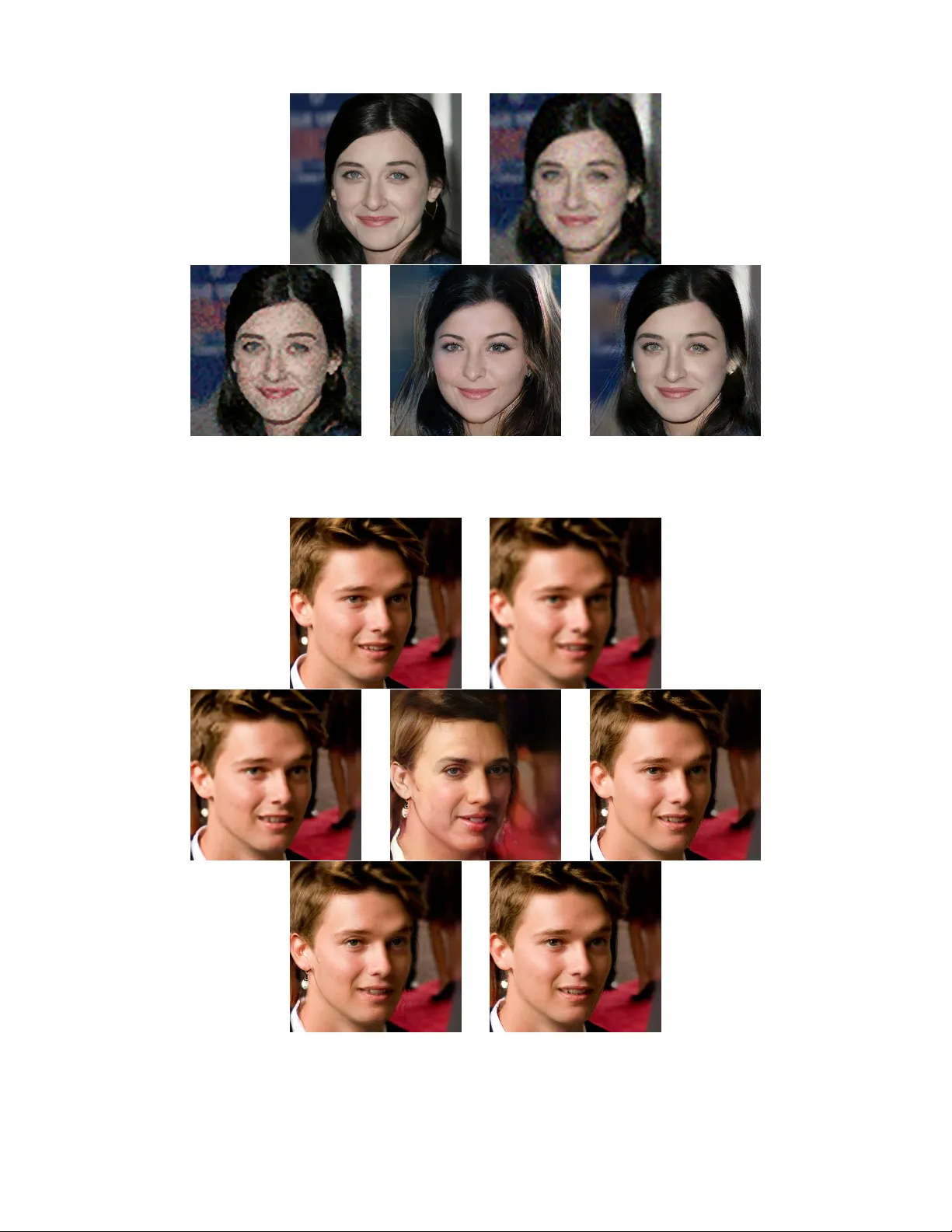
Image-Adaptiv e GAN based Reconstruction Shady Abu Hussein ∗ , T om Tir er ∗ , and Raja Giryes School of Electrical Engineering T el A vi v Uni versity , T el A vi v , Israel Abstract In the recent years, there has been a significant improvement in the quality of samples produced by (deep) generativ e mod- els such as v ariational auto-encoders and generative adversar - ial networks. Howe ver, the representation capabilities of these methods still do not capture the full distribution for complex classes of images, such as human faces. This deficiency has been clearly observed in previous works that use pre-trained generativ e models to solve imaging inv erse problems. In this paper , we suggest to mitigate the limited representation ca- pabilities of generators by making them image-adapti ve and enforcing compliance of the restoration with the observations via back-projections. W e empirically demonstrate the advan- tages of our proposed approach for image super-resolution and compressed sensing. Introduction The dev elopments in deep learning (Goodfello w , Bengio, and Courville 2016) in the recent years have led to signif- icant improvement in learning generative models. Methods like v ariational auto-encoders (V AEs) (Kingma and W elling 2013), generati ve adversarial networks (GANs) (Goodfel- low et al. 2014) and latent space optimizations (GLOs) (Bojanowski et al. 2018) ha ve found success at modeling data distrib utions. Howe ver , for complex classes of images, such as human faces, while these methods can generate nice examples, their representation capabilities do not cap- ture the full distrib ution. This phenomenon is sometimes re- ferred to in the literature, especially in the context of GANs, as mode collapse (Arjovsk y , Chintala, and Bottou 2017; Karras et al. 2017). Y et, as demonstrated in (Richardson and W eiss 2018), it is common to other recent learning ap- proaches as well. Another line of works that has gained a lot from the de- velopments in deep learning is imaging in verse problems, where the goal is to recover an image x from its degraded or compressed observ ations y (Bertero and Boccacci 1998). Most of these w orks ha ve been focused on training a con vo- lutional neural network (CNN) to learn the in v erse mapping ∗ The authors have contributed equally to this work. Code is av ailable at https://github .com/shadyabh/IAGAN Copyright c  2020, Association for the Advancement of Artificial Intelligence (www .aaai.org). All rights reserved. from y to x for a specific observ ation model (e.g. super- resolution with certain scale factor and bicubic anti-aliasing kernel (Dong et al. 2014)). Y et, recent works ha ve suggested to use neural networks for handling only the image prior in a way that does not require exhausti ve offline training for each dif ferent observ ation model. This can be done by using CNN denoisers (Zhang et al. 2017; Meinhardt et al. 2017; Rick Chang et al. 2017) plugged into iterati ve optimization schemes (V enkatakrishnan, Bouman, and W ohlberg 2013; Metzler , Maleki, and Baraniuk 2016; Tirer and Giryes 2018), training a neural netw ork from scratch for the imag- ing task directly on the test image (based on internal recur- rence of information inside a single image) (Shocher , Cohen, and Irani 2018; Ulyanov , V edaldi, and Lempitsky 2018), or using generati ve models (Bora et al. 2017; Y eh et al. 2017; Hand, Leong, and V oroninski 2018). Methods that use generati ve models as priors can only handle images that belong to the class or classes on which the model was trained. Ho we ver , the generati ve learning equips them with valuable semantic information that other strategies lack. For example, a method which is not based on a generativ e model cannot produce a perceptually pleas- ing image of human face if the e yes are completely missing in an inpainting task (Y eh et al. 2017). The main drawback in restoring complex images using generativ e models is the limited representation capabilities of the generators. Even when one searches over the range of a pre-trained generator for an image which is closest to the original x , he is expected to get a significant mismatch (Bora et al. 2017). In this work, we propose a strategy to mitigate the lim- ited representation capabilities of generators when solving in v erse problems. The strategy is based on a gentle internal learning phase at test time, which essentially makes the gen- erator image-adaptiv e while maintaining the useful informa- tion obtained in the of fline training. In addition, in scenarios with lo w noise le vel, we propose to further improve the re- construction by a back-projection step that strictly enforces compliance of the restoration with the observations y . W e empirically demonstrate the adv antages of our proposed ap- proach for image super-resolution and compressed sensing. Related W ork Our work is mostly related to the work by Bora et al. (2017), which hav e suggested to use pre-trained generativ e mod- els for the compressive sensing (CS) task (Donoho 2006; Candes, Romber g, and T ao 2006): reconstructing an un- known signal x ∈ R n from observations y ∈ R m of the form y = Ax + e , (1) where A is an m × n measurement matrix, e ∈ R m rep- resents the noise, and the number of measurements is much smaller than the ambient dimension of the signal, i.e. m  n . Follo wing the fact that in highly popular generati ve mod- els (e.g. GANs, V AEs and GLOs) a generator G ( · ) learns a mapping from a lo w dimensional space z ∈ R k to the sig- nal space G ( z ) ⊂ R n , the authors (Bora et al. 2017) hav e proposed a method, termed CSGM, that estimates the sig- nal as ˆ x = G ( ˆ z ) , where ˆ z is obtained by minimizing the non-con v ex 1 cost function f ( z ) = k y − AG ( z ) k 2 2 , (2) using backpropagation and standard gradient based optimiz- ers. For specific classes of images, such as handwritten dig- its and human faces, the experiments in (Bora et al. 2017; Hand, Leong, and V oroninski 2018) have shown that us- ing learned generati ve models enables to reconstruct nice looking images with much fewer measurements than meth- ods that use non-generati v e (e.g. model-based) priors. How- ev er , unlike the latter , it has been also shown that CSGM and its variants cannot pro vide accurate recov ery e v en when there is no noise and the number of observations is very large. This shortcoming is mainly due to the limited rep- resentation capabilities of the generativ e models (see Sec- tion 6.3 in (Bora et al. 2017)), and is common to related recent works (Hand, Leong, and V oroninski 2018; Bora, Price, and Dimakis 2018; Dhar, Grov er , and Ermon 2018; Shah and Hegde 2018). Note that using specific structures of A , the model (1) can be used for different imaging in verse problems, making the CSGM method applicable for these problems as well. For example, it can be used for denoising task when A is the n × n identity matrix I n , inpainting task when A is an m × n sampling matrix (i.e. a selection of m rows of I n ), deblurring task when A is a blurring operator , and super- resolution task if A is a composite operator of blurring (i.e. anti-aliasing filtering) and down-sampling. Our image-adaptiv e approach is inspired by (T irer and Giryes 2019), which is influenced itself by (Shocher, Cohen, and Irani 2018; Ulyanov , V edaldi, and Lempitsky 2018). These works follow the idea of internal recurrence of in- formation inside a single image within and across scales (Glasner , Bagon, and Irani 2009). Howe ver , while the two methods (Shocher , Cohen, and Irani 2018; Ulyanov , V edaldi, and Lempitsky 2018) completely avoid an offline training phase and optimize the weights of a deep neural network 1 The function f ( z ) is non-con vex due to the non-con ve xity of G ( z ) . only in the test phase, the work in (T irer and Giryes 2019) incorporates external and internal learning by taking of- fline trained CNN denoisers, fine-tuning them in test time and then plugging them into a model-based optimization scheme (Tirer and Giryes 2018). Note, though, that the in- ternal learning phase in (T irer and Giryes 2019) uses patches from y as the ground truth for a denoising loss function ( f ( ˜ x ) = k y − ˜ x k 2 2 ), building on the assumption that y di- rectly includes patterns which recur also in x . Therefore, this method requires that y is not very degraded, which makes it suitable perhaps only for the super -resolution task, similarly to (Shocher , Cohen, and Irani 2018), which is also restricted to this problem. Note that the method in (Ulyanov , V edaldi, and Lempit- sky 2018), termed as deep image prior (DIP), can be applied to dif ferent observ ation models. Ho we ver , the advantage of our approach stems from the offline generati v e learning that captures valuable semantic information that DIP lacks. As mentioned above, a method like DIP , which is not based on a generati ve model, cannot produce a perceptually pleasing image of human face if the eyes are completely missing in an inpainting task (Y eh et al. 2017). In this paper , we demon- strate that this adv antage holds also for highly ill-posed sce- narios in image super-resolution and compressed sensing. In addition, note that the DIP approach typically works only with huge U-Nets like architectures that need to be modified for each in verse problem and require much more memory than common generators. Indeed, we struggled (GPU mem- ory overflo w , long run-time) to apply DIP to the 1024 × 1024 images of CelebA-HQ dataset (Karras et al. 2017). The Proposed Method In this work, our goal is to make the solutions of in verse problems using generativ e models more faithful to the ob- servations and more accurate, despite the limited represen- tation capabilities of the pre-trained generators. T o this end, we propose an image-adapti ve approach, whose motiv ation is explained both v erbally and mathematically (building on theoretical results from (Bora et al. 2017)). W e also dis- cuss a back-projection post-processing step that can fur- ther improve the results for scenarios with low noise level. While this post-processing, typically , only moderately im- prov es the results of model-based super-resolution algo- rithms (Glasner, Bagon, and Irani 2009; Y ang et al. 2010), we will show that it is highly effecti v e for generativ e priors. T o the best of our knowledge, we are the first to use it in reconstructions based on generativ e priors. An Image-Adaptive Appr oach W e propose to handle the limited representation capabilities of the generators by making them image-adaptive (IA) us- ing internal learning in test-time. In details, instead of re- cov ering the latent signal x as ˆ x = G ( ˆ z ) , where G ( · ) is a pre-trained generator and ˆ z is a minimizer of (2), we sug- gest to simultaneously optimize z and the parameters of the generator , denoted as θ , by minimizing the cost function f I A ( θ , z ) = k y − A G θ ( z ) k 2 2 . (3) The optimization is done using backpropagation and stan- dard gradient based optimizers. The initial value of θ is the pre-trained weights, and the initial value of z is ˆ z , obtained by minimization with respect to z alone, as done in CSGM. Then, we perform joint-minimization to obtain ˆ θ I A and ˆ z I A , and recov er the signal using ˆ x I A = G ˆ θ I A ( ˆ z I A ) . The rationale behind our approach can be explained as follows. Current leading learning strategies cannot train a generator whose representation range cov ers every sam- ple of a complex distribution, thus, optimizing only z is not enough. Howe ver , the expressi v e power of deep neu- ral networks (giv en by optimizing the weights θ as well) allows to create a single specific sample that agrees with the observations y . Y et, contrary to prior works that opti- mize the weights of neural networks only by internal learn- ing (Shocher , Cohen, and Irani 2018; Ulyanov , V edaldi, and Lempitsky 2018), here we incorporate information captured in the test-time with the valuable semantic knowledge ob- tained by the offline generati ve learning. T o make sure that the information captured in test-time does not come at the expense of of fline information which is useful for the test image at hand , we start with optimiz- ing z alone, as mentioned above, and then apply the joint minimization with a small learning rate and early stopping (details in the experiments section belo w). Mathematical Motivation for Image-Adaptation T o moti v ate the image-adapti ve approach, let us consider an L -layer neural network generator G ( z ; { W ` } L ` =1 ) = W L σ ( W L − 1 σ ( . . . σ ( W 1 z ) . . . )) , (4) where σ ( · ) denotes element-wise ReLU acti v ation, and W ` ∈ R k ` × k ` − 1 such that k L = n . Recall that typically k 0 < k 1 < . . . < k L (as k 0  n ). The following theorem, which has been proven in (Bora et al. 2017) (Theorem 1.1 there), provides an upper bound on the reconstruction error . Theorem 1. Let G ( z ) : R k → R n as given in (4) , A ∈ R m × n with A ij ∼ N (0 , 1 /m ) , m = Ω ( k L log n ) , and y = Ax + e . Let ˆ z minimize k y − AG ( z ) k 2 to within additive  of the optimum. Then, with pr obability 1 − e − Ω( m ) we have k G ( ˆ z ) − x k 2 ≤ 6 E rep ( G ( · ) , x ) + 3 k e k 2 + 2 , (5) wher e E rep ( G ( · ) , x ) := min z k G ( z ) − x k 2 . Note that E rep ( G ( · ) , x ) is in f act the representation error of the generator for the specific image x . This term has been empirically observed in (Bora et al. 2017) to dominate the ov erall error , e.g. more than the error of the optimization al- gorithm (represented by  ). The following proposition builds on Theorem 1 and motiv ates the joint optimization of z and W 1 by guaranteeing a decreased representation error term. Proposition 2. Consider the generator defined in (4) with k 0 < k 1 , A ∈ R m × n with A ij ∼ N (0 , 1 /m ) , m = Ω ( k 1 L log n ) , and y = Ax + e . Let ˆ z and ˆ W 1 minimize ˜ f ( z , W 1 ) = k y − AG ( z ; { W ` } L ` =1 ) k 2 to within additive  of the optimum. Then, with pr obability 1 − e − Ω( m ) we have k G ( ˆ z ; ˆ W 1 , { W ` } L ` =2 ) − x k 2 ≤ 6 ˜ E rep + 3 k e k 2 + 2 , (6) wher e ˜ E rep ≤ E rep ( G ( · ) , x ) . Pr oof. Define ˆ ˜ z := ˆ W 1 ˆ z and ˜ G ( ˜ z ) := W L σ ( W L − 1 σ ( . . . σ ( W 2 σ ( I k 1 ˜ z )) . . . )) . Note that G ( ˆ z ; ˆ W 1 , { W ` } L ` =2 ) = ˜ G ( ˆ ˜ z ) , therefore ˆ ˜ z minimize k y − A ˜ G ( ˜ z ) k 2 to within additi ve  of the optimum. Applying Theorem 1 on ˜ G ( ˜ z ) and ˆ ˜ z we hav e k ˜ G ( ˆ ˜ z ) − x k 2 ≤ 6 E rep ( ˜ G ( · ) , x ) + 3 k e k 2 + 2 , (7) with the advertised probability . No w , note that E rep ( ˜ G ( · ) , x ) = min ˜ z ∈ R k 1 k W L σ ( W L − 1 σ ( . . . σ ( W 2 σ ( I k 1 ˜ z )) . . . )) − x k 2 ≤ min z ∈ R k 0 k W L σ ( W L − 1 σ ( . . . σ ( W 2 σ ( W 1 z )) . . . )) − x k 2 = E rep ( G ( · ) , x ) , (8) where the inequality follo ws from W 1 R k 0 ⊂ R k 1 . W e finish with substituting ˜ G ( ˆ ˜ z ) = G ( ˆ z ; ˆ W 1 , { W ` } L ` =2 ) in (7) and defining ˜ E rep := E rep ( ˜ G ( · ) , x ) . Proposition 2 shows that under the mathematical frame- work of Theorem 1, and under the (reasonable) assumption that the output dimension of the first layer is larger than its input, it is possible to further reduce the representation error of the generator for x (the term that empirically dominates the ov erall error) by optimizing the weights of the first layer as well. The result follows from obtaining an increased set in which the nearest neighbor of x is searched. Note that if k 0 < k 1 < . . . < k L , then the procedure which is described in Proposition 2 can be repeated sequen- tially layer after layer to further reduce the representation error . Howe ver , note that this theory loses its meaningful- ness at high layers because m = Ω ( k ` L log n ) approaches Ω ( n ) (so no prior is necessary). Y et, it presents a moti v ation to optimize all the weights, as we suggest to do in practice. ”Hard” vs. ”Soft” Compliance to Observations The image-adaptiv e approach improv es the agreement be- tween the recovery and the observations. W e turn now to describe another complementary way to achie ve this goal. Denote by ˆ x an estimation of x , e.g. using CSGM method or our IA approach. Assuming that there is no noise, i.e. e = 0 , a simple post-processing to strictly enforce compliance of the restoration with the observations y is back-projecting (BP) the estimator ˆ x onto the af fine subspace { A R n = y } ˆ x bp = argmin ˜ x k ˜ x − ˆ x k 2 2 s.t. A ˜ x = y . (9) Note that this problem has a closed-form solution ˆ x bp = A † y + ( I n − A † A ) ˆ x = A † ( y − A ˆ x ) + ˆ x , (10) where A † := A T ( AA T ) − 1 is the pseudoinv erse of A (as- suming that m < n , which is the common case, e.g. in super- resolution and compressed sensing tasks). In practical cases, Figure 1: Compressed sensing with Gaussian measurement matrix using BEGAN. From left to right and top to bottom: original image, CSGM for m/n = 0 . 122 , CSGM-BP for m/n = 0 . 122 , CSGM for m/n = 0 . 61 , CSGM-BP for m/n = 0 . 61 , IA GAN for m/n = 0 . 122 , IA GAN-BP for m/n = 0 . 122 , IA GAN for m/n = 0 . 61 , IA GAN-BP for m/n = 0 . 61 . Figure 2: Compressed sensing with Gaussian measurement matrix using BEGAN. Reconstruction MSE (averaged over 100 images from CelebA) vs. the compression ratio m/n . where the problem dimensions are high, the matrix in v er- sion in A † can be av oided by using the conjugate gradient method (Hestenes and Stiefel 1952). Note that when y is noisy , the operation A † y in (10) is e xpected to amplify the noise. Therefore, the BP post-processing is useful as long as the noise lev el is lo w . Let P A := A † A denote the orthogonal projection onto the ro w space of A , and Q A := I n − A † A denote its or- thogonal complement. Substituting (1) into (10) giv es ˆ x bp = P A x + Q A ˆ x + A † e , (11) which shows that ˆ x bp is consistent with y on P A x (i.e. dis- plays ”hard” compliance ), and considers only the projection of ˆ x onto the null space of A . Therefore, for an estimate ˆ x obtained via a generativ e model, the BP technique essen- tially eliminates the component of the generator’ s represen- tation error that resides in the ro w space of A , but does not change at all the component in the null space of A . Still, from the (Euclidean) accuracy point of view , this strategy is very ef fecti ve at lo w noise le vels, as demonstrated in the experiments section. Interestingly , note that our image-adapti ve strategy en- forces only a ”soft” compliance of the restoration with the observations y , because our gentle joint optimization (which prev ents overriding the offline semantic information) may not completely diminish the component of the generator’ s representation error that resides in the row space of A , as done by BP . On the other hand, intuitiv ely , the strong prior (imposed by the of fline training and by the generator’ s struc- ture) is expected to improve the restoration also in the null space of A (unlike BP). Indeed, as sho wn belo w , by com- bining the two approaches, i.e. applying the IA phase and then the BP on ˆ x I A , we obtain better results than only ap- plying BP on CSGM. This ob viously implies decreasing the component of reconstruction error in the null space of A . Experiments In our experiments we use two recently proposed GAN mod- els, which are kno wn to generate v ery high quality samples of human faces. The first is BEGAN (Berthelot, Schumm, and Metz 2017), trained on CelebA dataset (Liu et al. 2015), which generates a 128 × 128 image from a uniform random vector z ∈ R 64 . The second is PGGAN (Karras et al. 2017), trained on CelebA-HQ dataset (Karras et al. 2017) that gen- erates a 1024 × 1024 image from a Gaussian random v ector z ∈ R 512 . W e use the official pre-trained models, and for de- tails on the models and their training procedures we refer the reader to the original publications. Note that previous works, which use generativ e models for solving in verse problems, hav e considered much simpler datasets, such as MNIST (Le- Cun et al. 1998) or a small version of CelebA (do wnscaled to size 64 × 64 ), which perhaps do not demonstrate how se vere the effect of mode collapse is. The test-time procedure is done as follows, and is almost the same for the tw o models. F or CSGM we follo w (Bora et al. 2017) and optimize (2) using AD AM optimizer (Kingma and Ba 2014) with learning rate (LR) of 0.1. W e use 1600 iterations for BEGAN and 1800 iterations for PGGAN. The final z , i.e. ˆ z , is chosen to be the one with minimal objecti ve value f ( z ) along the iterations, and the CSGM recovery is ˆ x = G ( ˆ z ) . Performing a post-processing BP step (10) gi ves us also a reconstruction that we denote by CSGM-BP . In the reconstruction based on image-adaptive GANs, Figure 3: Compressed sensing with 30% (top) and 50% (bot- tom) subsampled Fourier measurements and noise lev el of 10/255, for CelebA images. Left to right: original image, naiv e reconstruction (zero padding and IFFT), DIP , CSGM, and IA GAN. CSGM and IA GAN use the BEGAN prior . which we denote by IA GAN, we initialize z with ˆ z , and then optimize (3) jointly for z and θ (the generator parameters). For BEGAN we use LR of 10 − 4 for both z and θ in all scenarios, and for PGGAN we use LR of 10 − 4 and 10 − 3 for z and θ , respecti vely . For BEGAN, we use 600 itera- tions for compressed sensing and 500 for super-resolution. For PGGAN we use 500 and 300 iterations for compressed sensing and super-resolution, respectiv ely . In the examined noisy scenarios we use only half of the amount of iterations, to av oid overfitting the noise. The final minimizers ˆ θ I A and ˆ z I A are chosen according to the minimal objectiv e value, and the IA GAN result is obtained by ˆ x I A = G ˆ θ I A ( ˆ z I A ) . Another recov ery , which uses also the post-processing BP step (10) on ˆ x I A , is denoted by IA GAN-BP . W e also compare the methods with DIP (Ulyanov , V edaldi, and Lempitsky 2018). W e use DIP official imple- mentation for the noiseless scenarios, and for the examined noisy scenarios we reduce the number of iterations by a fac- tor of 4 (tuned for best av erage performance) to prev ent the network from ov erfitting the noise. Apart from presenting visual results 2 , we compare the performance of the different methods using tw o quantitati ve measures. The first one is the widely-used mean squared er- ror (MSE) (sometimes in its PSNR form 3 ). The second is a distance between images that focuses on perceptual similar - ity (PS), which has been proposed in (Zhang et al. 2018) (we use the official implementation). Displaying the PS is impor - tant since it is well known that PSNR/MSE may not corre- late with the visual/perceptual quality of the reconstruction. Note that in the PS score — lower is better . Compressed Sensing In the first experiment we demonstrate ho w the proposed IA and BP techniques significantly outperform or improve upon CSGM for a large range of compression ratios. W e consider noiseless compressed sensing using an m × n Gaussian ma- trix A with i.i.d. entries drawn from A ij ∼ N (0 , 1 /m ) , sim- 2 More visual examples are presented in Figures 11 - 12 for com- pressed sensing and in Figures 13 - 16 for super-resolution. 3 W e compute the a verage PSNR as 10log 10 (255 2 / MSE) , where MSE is av eraged over the test images. Figure 4: Compressed sensing with 30% (top group) and 50% (bottom group) subsampled Fourier measurements and noise lev el of 10/255, for CelebA-HQ images. From left to right and top to bottom: original image, naiv e reconstruction (zero padding and IFFT), DIP , CSGM, and IA GAN. Note that CSGM and IA GAN use the PGGAN prior . ilar to the experiments in (Bora et al. 2017). In this case, there is no efficient way to implement the operators A and A T . Therefore, we consider only the BEGAN that generates 128 × 128 images (i.e. n = 3 × 128 2 = 49 , 152 ), which are much smaller than those generated by PGGAN. Figure 1 shows sev eral visual results and Figure 2 presents the reconstruction MSE of the different methods as we change the number of measurements m (i.e. we change the compression ratio m/n ). The results are averages ov er 20 images from CelebA dataset. It is clearly seen that IAGAN outperforms CSGM for all the values of m . Note that due to the limited representation capabilities of BEGAN (equi v- alently – its mode collapse), CSGM performance reaches a Figure 5: Binary masks for compressed sensing with 30% (left) and 50% (right) subsampled Fourier measurements. T able 1: Compressed sensing with subsampled Fourier mea- surements. Reconstruction PSNR [dB] (left) and PS (Zhang et al. 2018) (right), a veraged over 100 images from CelebA and CelebA-HQ, for compression ratios 0.3 and 0.5, with noise lev el of 10/255. CelebA naiv e IFFT DIP CSGM IA GAN CS ratio 0.3 19.23 / 0.540 25.96 / 0.139 20.12 / 0.246 25.50 / 0.092 CS ratio 0.5 20.53 / 0.495 27.21 / 0.125 20.32 / 0.241 27.59 / 0.066 CelebA-HQ naiv e IFFT DIP CSGM IA GAN CS ratio 0.3 19.65 / 0.625 24.97 / 0.566 21.38 / 0.520 25.80 / 0.429 CS ratio 0.5 20.45 / 0.597 26.29 / 0.535 21.82 / 0.514 28.26 / 0.378 Figure 6: Super-resolution with scale factor 4, bicubic ker - nel, and no noise, for CelebA images. From left to right and top to bottom: original image, bicubic upsampling, DIP , CSGM, CSGM-BP , IA GAN, and IA GAN-BP . Note that CSGM and IA GAN use the BEGAN prior . plateau in a quite small v alue of m , contrary to IA GAN er- ror that continues to decrease. The back-projection strate gy is sho wn to be v ery ef fecti ve, as it makes sure that CSGM- BP is rescued from the plateau of CSGM. The f act that IA- GAN still has a very small error when the compression ratio is almost 1 follows from our small learning rates and early stopping, which ha ve been found necessary for small values of m , where the null space of A is very large and it is im- portant to a v oid o verriding the of fline semantic information. Howe ver , this small error is often barely visible, as demon- strated by visual results in Figure 1, and further decreases by the BP step of IA GAN-BP . In order to examine our proposed IA strategy for the larger model PGGAN as well, we turn to use a different measurement operator A which can be applied ef ficiently – the subsampled Fourier transform. This acquisition model is also more common in practice, e.g. in sparse MRI (Lustig, Donoho, and P auly 2007). W e consider scenarios with com- pression ratios of 0.3 and 0.5, and noise level of 10/255 (due to the noise we do not apply the BP post-processing). The PSNR and PS results (av eraged on 100 images from each dataset) are given in T able 1, and sev eral visual examples are shown in Figures 3 and 4. In Figure 5 we present the bi- nary masks used for 30% and 50% Fourier domain sampling of 128 × 128 images in CelebA. The binary masks that ha ve been used for CelebA-HQ hav e similar forms. Figure 7: Super-resolution with bicubic kernel, scale factor 8, and noise level of 10/255, for CelebA-HQ images. From left to right and top to bottom: original image, bicubic up- sampling, DIP , CSGM, and IA GAN. Note that CSGM and IA GAN use the PGGAN prior . Figure 8: Super-resolution with bicubic kernel, scale fac- tor 16, and no noise, for CelebA-HQ images. From left to right and top to bottom: original image, bicubic upsampling, DIP , CSGM, IA GAN, CSGM-BP , and IA GAN-BP . Note that CSGM and IA GAN use the PGGAN prior . T able 2: Super-resolution with bicubic downscaling kernel. Reconstruction PSNR [dB] (left) and PS (Zhang et al. 2018) (right), av eraged ov er 100 images from CelebA and CelebA-HQ, for scale factors 4, 8 and 16, with no noise. CelebA Bicubic DIP CSGM CSGM-BP IA GAN IA GAN-BP SR x4 26.50 / 0.165 27.35 / 0.159 20.51 / 0.235 26.44 / 0.165 27.16 / 0.092 27.14 / 0.092 SR x8 22.39 / 0.212 23.45 / 0.339 20.23 / 0.240 22.71 / 0.212 23.49 / 0.158 23.53 / 0.157 CelebA-HQ Bicubic DIP CSGM CSGM-BP IA GAN IA GAN-BP SR x8 29.94 / 0.398 30.01 / 0.400 22.62 / 0.505 28.54 / 0.398 28.76 / 0.387 28.76 / 0.360 SR x16 27.43 / 0.437 27.51 / 0.480 22.34 / 0.506 26.20 / 0.437 26.28 / 0.421 25.86 / 0.411 T able 3: Super-resolution with bicubic do wnscaling kernel. Reconstruction PSNR [dB] (left) and PS (Zhang et al. 2018) (right), averaged over 100 images from CelebA and CelebA- HQ, for scale factors 4, 8 and 16, with noise le vel of 10/255. CelebA Bicubic DIP CSGM IA GAN SR x4 24.72 / 0.432 24.19 / 0.280 20.57 / 0.238 25.54 / 0.133 SR x8 21.65 / 0.660 21.22 / 0.513 20.22 / 0.243 21.72 / 0.243 CelebA-HQ Bicubic DIP CSGM IAGAN SR x8 26.31 / 0.801 27.61 / 0.430 21.60 / 0.519 26.30 / 0.421 SR x16 25.02 / 0.781 24.20 / 0.669 21.31 / 0.516 24.73 / 0.455 The unsatisfactory results obtained by CSGM clearly demonstrate the limited capabilities of both BEGAN and PGGAN for reconstruction: Despite the fact that both of them can generate very nice samples (Berthelot, Schumm, and Metz 2017; Karras et al. 2017), they typically can- not represent well an image that fits the gi ven observ ations y . This is resolved by our image-adapti ve approach. For CelebA dataset DIP has competitiv e PSNR with our IA- GAN. Howe ver , both the qualitative examples and the PS (perceptual similarity) measure agree that IA GAN results are much more pleasing. For CelebA-HQ dataset our IA- GAN clearly outperforms the other methods. Inference run-time. Since IAGAN performs a quite small number of ADAM iterations to jointly optimize z and θ (the generator’ s parameters), it requires only a small addi- tional time compared to CSGM. Y et, both methods are much faster than DIP , which trains from scratch a large CNN at test-time. For example, for compression ratio of 0.5, using NVIDIA R TX 2080ti GPU we got the follo wing per im- age run-time: for CelebA: DIP ∼ 100s, CSGM ∼ 30s, and IA GAN ∼ 35s; and for CelebA-HQ: DIP ∼ 1400s, CSGM ∼ 120s, and IA GAN ∼ 140s. The same behavior , i.e. CSGM and IAGAN are much f aster than DIP , holds throughout the experiments in the paper (e.g. also for the super-resolution task). Super -Resolution W e turn to examine the super-resolution task, for A which is a composite operator of blurring with a bicubic anti-aliasing kernel followed by down-sampling. For BEGAN we use super-resolution scale factors of 4 and 8, and for PGGAN we use scale factors of 8 and 16. W e check a noiseless scenario Figure 9: Super-resolution of misaligned images with bicu- bic kernel and scale factor 4 using BEGAN. Left to right: original image, bicubic upsampling, CSGM, and IA GAN. and a scenario with noise le vel of 10/255. For the noiseless scenario we also examine the GAN-based recovery after a BP post-processing, which can be computed ef ficiently , be- cause A † can be implemented by bicubic upsampling. The PSNR and PS results (av eraged on 100 images from each dataset) of the different methods are gi ven in T ables 2 and 3, and sev eral visual e xamples are shown in Figures 6 - 8. Once again, the results of the plain CSGM are not satis- fying. Due to the limited representation capabilities of BE- GAN and PGGAN, the recovered faces look very different than the ones in the test images. The BP post-processing is very effecti ve in reducing CSGM representation error when the noise lev el is minimal. For our IA GAN approach, the BP step is less ef fective (i.e. IA GAN and IA GAN-BP ha v e sim- ilar reco veries), which implies that the ”soft-compliance” of IA GAN obtains similar results as the ”hard-compliance” of the BP in the ro w space of A . In the noiseless case, DIP of- ten obtains better PSNR than IA GAN. Ho we ver , as observ ed in the compressed sensing experiments, both the visual ex- amples and the PS (perceptual similarity) measure agree that IA GAN results are much more pleasing and sharper , in both noisy and noiseless scenarios. A similar tradeoff between distortion and perception has been recently in vestigated by Blau and Michaeli (2018). Their work supports the obser- vation that the balance between fitting the measurements and preserving the generative prior , which is the core of our IA GAN approach, may limit the achie v able PSNR in some cases but significantly impro ves the perceptual quality . W e finish this section with an extreme demonstration of mode collapse. In this scenario we use the BEGAN model to super-resolv e images with scale factor of 4. Y et, this time the T able 4: Deblurring with 9 × 9 uniform filter and noise le v el of 10/255. Reconstruction PSNR [dB] (left) and PS (Zhang et al. 2018) (right), a veraged over 100 images from CelebA and CelebA-HQ. CelebA Blurred DIP CSGM IA GAN Deb U(9x9) 22.21 / 0.490 25.63 / 0.203 20.37 / 0.241 26.15 / 0.110 CelebA-HQ Blurred DIP CSGM IA GAN Deb U(9x9) 25.80 / 0.622 28.28 / 0.458 21.62 / 0.507 28.25 / 0.388 images are slightly misaligned — they are vertically trans- lated by a fe w pixels. The PSNR[dB] / PS results (av eraged on 100 CelebA images) are 19.18 / 0.374 for CSGM and 26.73 / 0.127 for IA GAN. Sev eral visual results are shown in Figure 9. The CSGM is highly susceptible to the poor ca- pabilities of BEGAN in this case, while our IA GAN strategy is quite robust. Deblurring W e briefly demonstrate that the advantage of IA GAN car- ries to more in verse problems by examining a deblurring scenario, where the operator A represents blurring with a 9 × 9 uniform filter , and the noise le vel is 10/255 (so we do not apply the BP post-processing). The PSNR and PS results (av eraged on 100 images from each dataset) of DIP , CSGM, and IA GAN are giv en in T able 4, and se veral visual exam- ples are presented in Figure 10. Similarly to the previous experiments, the proposed IA- GAN often exhibits the best PSNR and consistently exhibits the best perceptual quality . Conclusion In this work we considered the usage of generative models for solving imaging in v erse problems. The main deficiency in such applications is the limited representation capabilities of the generators, which unfortunately do not capture the full distribution for complex classes of images. W e suggested two strategies for mitigating this problem. One technique is a post-processing back-projection step, which is applica- ble at low noise lev el, that essentially eliminates the com- ponent of the generator’ s representation error that resides in the row space of the measurement matrix. The second tech- nique, which is our main contrib ution, is an image adaptiv e approach, termed IAGAN, that improv es the generator capa- bility to represent the specific test image. This method can improv e also the restoration in the null space of the measure- ment matrix. One can also use the two strategies together . Experiments on compressed sensing and super-resolution tasks demonstrated that our strate gies, especially the image- adaptiv e approach, yield significantly impro ved reconstruc- tions, which are both more accurate and perceptually pleas- ing than other alternativ es. Acknowledgments This work is partially supported by the NSF-BSF grant (No. 2017729) and the European re- search council (ERC StG 757497 PI Giryes). Figure 10: Deblurring with 9 × 9 uniform filter and noise lev el of 10/255, for CelebA-HQ images. From left to right and top to bottom (in each group): original image, blurred and noisy image, DIP , CSGM, and IA GAN. Note that CSGM and IA GAN use the PGGAN prior . References Abu Hussein, S.; Tirer , T .; and Giryes, R. 2019. Image- adaptiv e GAN based reconstruction. arXiv pr eprint arXiv:1906.05284 . Arjovsk y , M.; Chintala, S.; and Bottou, L. 2017. W asser- stein generati ve adversarial networks. In International Con- fer ence on Machine Learning , 214–223. Bertero, M., and Boccacci, P . 1998. Intr oduction to inver se pr oblems in imaging . CRC press. Berthelot, D.; Schumm, T .; and Metz, L. 2017. Be- gan: Boundary equilibrium generativ e adv ersarial networks. arXiv pr eprint arXiv:1703.10717 . Blau, Y ., and Michaeli, T . 2018. The perception-distortion tradeoff. In Pr oceedings of the IEEE Confer ence on Com- puter V ision and P attern Recognition , 6228–6237. Bojanowski, P .; Joulin, A.; Lopez-Pas, D.; and Szlam, A. 2018. Optimizing the latent space of generati ve networks. In International Confer ence on Machine Learning , 599–608. Bora, A.; Jalal, A.; Price, E.; and Dimakis, A. G. 2017. Compressed sensing using generativ e models. In Interna- tional Confer ence on Machine Learning , 537–546. Bora, A.; Price, E.; and Dimakis, A. G. 2018. Ambientgan: Generativ e models from lossy measurements. In Interna- tional Confer ence on Learning Repr esentations (ICLR) . Candes, E.; Romberg, J.; and T ao, T . 2006. Robust un- certainty principles: Exact signal reconstruction from highly incomplete frequency information. IEEE T ransactions on information theory 52(2):489–509. Dhar , M.; Grov er , A.; and Ermon, S. 2018. Modeling sparse deviations for compressed sensing using generativ e models. arXiv pr eprint arXiv:1807.01442 . Dong, C.; Loy , C. C.; He, K.; and T ang, X. 2014. Learning a deep con v olutional network for image super- resolution. In Eur opean conference on computer vision , 184–199. Springer . Donoho, D. 2006. Compressed sensing. IEEE T ransactions on information theory 52(4):1289–1306. Glasner , D.; Bagon, S.; and Irani, M. 2009. Super -resolution from a single image. In Computer V ision, 2009 IEEE 12th International Confer ence on , 349–356. IEEE. Goodfellow , I.; Bengio, Y .; and Courville, A. 2016. Deep learning . Goodfellow , I.; Pouget-Abadie, J.; Mirza, M.; Xu, B.; W arde-Farle y , D.; Ozair , S.; Courville, A.; and Bengio, Y . 2014. Generativ e adversarial nets. In Advances in neural information pr ocessing systems , 2672–2680. Hand, P .; Leong, O.; and V oroninski, V . 2018. Phase re- triev al under a generati ve prior . In Advances in Neural In- formation Pr ocessing Systems , 9154–9164. Hestenes, M. R., and Stiefel, E. 1952. Methods of conjugate gradients for solving linear systems , v olume 49. Karras, T .; Aila, T .; Laine, S.; and Lehtinen, J. 2017. Pro- gressiv e gro wing of gans for impro ved quality , stability , and variation. arXiv pr eprint arXiv:1710.10196 . Kingma, D. P ., and Ba, J. 2014. Adam: A method for stochastic optimization. arXiv pr eprint arXiv:1412.6980 . Kingma, D. P ., and W elling, M. 2013. Auto-encoding v ari- ational bayes. arXiv pr eprint arXiv:1312.6114 . LeCun, Y .; Bottou, L.; Bengio, Y .; Haf fner , P .; et al. 1998. Gradient-based learning applied to document recognition. Pr oceedings of the IEEE 86(11):2278–2324. Liu, Z.; Luo, P .; W ang, X.; and T ang, X. 2015. Deep learn- ing face attributes in the wild. In Pr oceedings of the IEEE international confer ence on computer vision , 3730–3738. Lustig, M.; Donoho, D.; and Pauly , J. M. 2007. Sparse MRI: The application of compressed sensing for rapid mr imaging. Magnetic Resonance in Medicine: An Of ficial Journal of the International Society for Magnetic Resonance in Medicine 58(6):1182–1195. Meinhardt, T .; Moller , M.; Hazirbas, C.; and Cremers, D. 2017. Learning proximal operators: Using denoising net- works for re gularizing inv erse imaging problems. In ICCV , 1781–1790. Metzler , C. A.; Maleki, A.; and Baraniuk, R. G. 2016. From denoising to compressed sensing. IEEE T ransactions on In- formation Theory 62(9):5117–5144. Richardson, E., and W eiss, Y . 2018. On GANs and GMMs. In Advances in Neural Information Pr ocessing Systems , 5852–5863. Rick Chang, J.; Li, C.-L.; Poczos, B.; V ijaya Kumar , B.; and Sankaranarayanan, A. C. 2017. One network to solve them all–solving linear in verse problems using deep projec- tion models. In ICCV , 5888–5897. Shah, V ., and Hegde, C. 2018. Solving linear in verse prob- lems using gan priors: An algorithm with provable guaran- tees. In 2018 IEEE International Confer ence on Acoustics, Speech and Signal Pr ocessing (ICASSP) , 4609–4613. IEEE. Shocher , A.; Cohen, N.; and Irani, M. 2018. ”zero-shot” super-resolution using deep internal learning. In CVPR . T irer , T ., and Giryes , R. 2018. Image restoration by iterati ve denoising and backward projections. IEEE T ransactions on Image Pr ocessing 28(3):1220–1234. T irer , T ., and Giryes, R. 2019. Super-resolution via image- adapted denoising CNNs: Incorporating external and inter- nal learning. IEEE Signal Pr ocessing Letters . Ulyanov , D.; V edaldi, A.; and Lempitsky , V . 2018. Deep image prior . In CVPR . V enkatakrishnan, S. V .; Bouman, C. A.; and W ohlber g, B. 2013. Plug-and-play priors for model based reconstruction. In Global Confer ence on Signal and Information Pr ocessing (GlobalSIP), 2013 IEEE , 945–948. IEEE. Y ang, J.; Wright, J.; Huang, T . S.; and Ma, Y . 2010. Image super-resolution via sparse representation. IEEE transac- tions on image pr ocessing 19(11):2861–2873. Y eh, R. A.; Chen, C.; Y ian Lim, T .; Schwing, A. G.; Hasega wa-Johnson, M.; and Do, M. N. 2017. Semantic image inpainting with deep generati v e models. In Pr oceed- ings of the IEEE Confer ence on Computer V ision and P at- tern Recognition , 5485–5493. Zhang, K.; Zuo, W .; Gu, S.; and Zhang, L. 2017. Learn- ing deep cnn denoiser prior for image restoration. In IEEE Confer ence on Computer V ision and P attern Recognition , 3929–3938. Zhang, R.; Isola, P .; Efros, A. A.; Shechtman, E.; and W ang, O. 2018. The unreasonable ef fecti veness of deep features as a perceptual metric. In Pr oceedings of the IEEE Confer ence on Computer V ision and P attern Recognition , 586–595. Figure 11: Compressed sensing using PGGAN with compression ratio of 30% and noise le v el of 10/255. From left to right and top to bottom: original image, naiv e reconstruction (zero padding and IFFT), DIP , CSGM, and IA GAN. Figure 12: Compressed sensing using PGGAN with compression ratio of 50% and noise le v el of 10/255. From left to right and top to bottom: original image, naiv e reconstruction (zero padding and IFFT), DIP , CSGM, and IA GAN. Figure 13: Super-resolution using PGGAN with scale factor of 8 without noise. From left to right and top to bottom: original image, bicubic upsampling, DIP , CSGM, IA GAN, CSGM-BP and IA GAN-BP . Figure 14: Super -resolution using PGGAN with scale factor of 8 and noise le vel of 10/255. From left to right and top to bottom: original image, bicubic upsampling, DIP , CSGM, and IA GAN. Figure 15: Super-resolution using PGGAN with scale factor of 16 and noise lev el of 10/255. From left to right and top to bottom: original image, bicubic upsampling, DIP , CSGM, and IA GAN. Figure 16: Super-resolution using PGGAN with scale factor of 16 without noise. From left to right and top to bottom: original image, bicubic upsampling, DIP , CSGM, IA GAN, CSGM-BP , and IA GAN-BP .