Technical report: supervised training of convolutional spiking neural networks with PyTorch

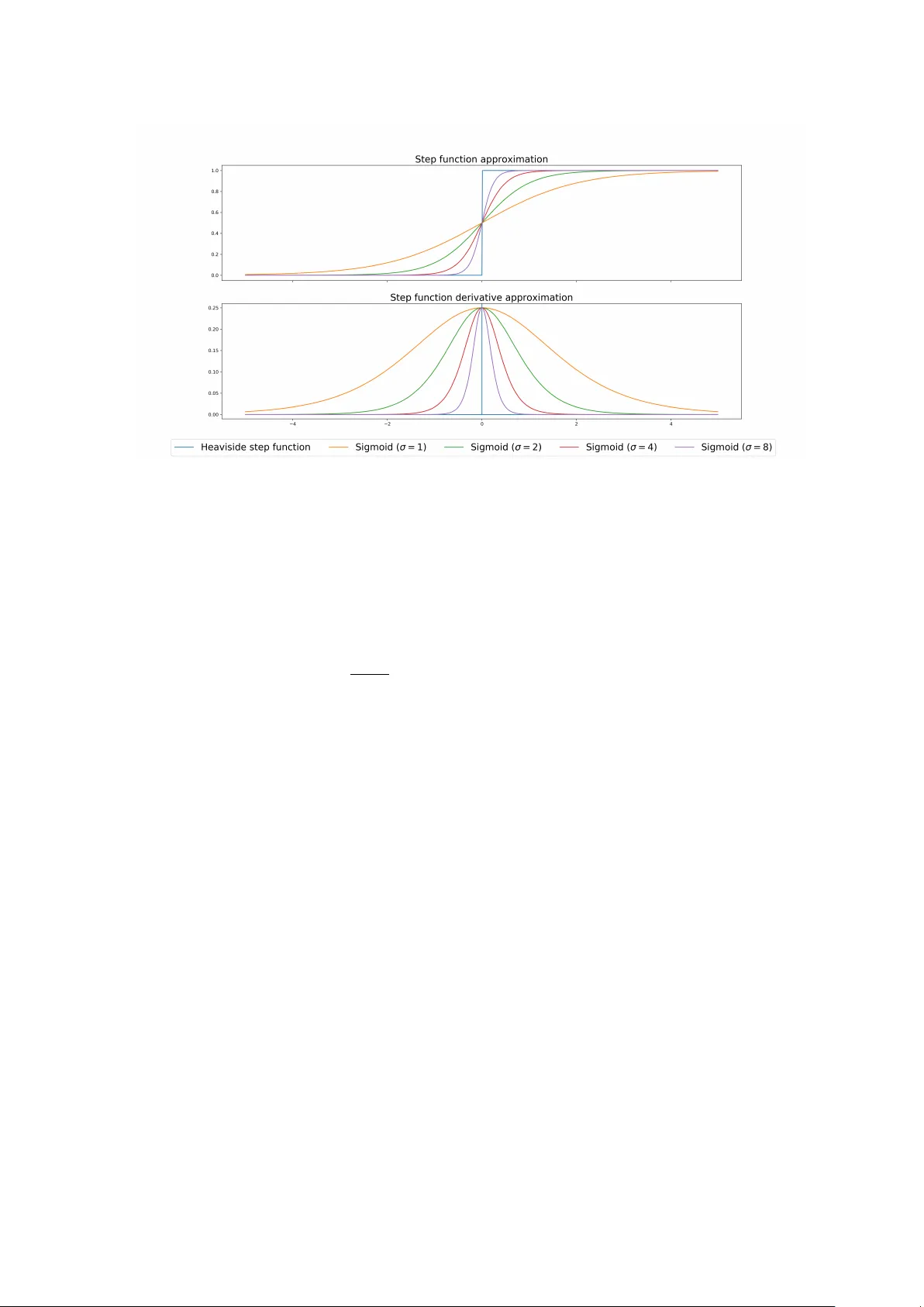
T echnical r eport: super vised training of convolutional spiking neur al networks with PyT or ch Romain Z immer 1, 2 , Thomas P ellegrini 2 , Srisht F ateh S ingh 1 , and T imothée Masquelier 1 1 CERC O UMR 5549, CNRS – Université T oulouse 3, T o ulouse , France 2 IRIT , Université de T oulouse, T oulouse, Fr ance Recently , it has been sho wn that spiking neural networks (SNNs) can be trained efficiently , in a supervised manner , using backpr opagation through time. In- deed, the most commonly used spiking neuron model, the leaky integrate-and- fire neuron, obeys a differ ential equation which can be approximated using dis- crete time steps, leading to a recurrent r elation for the potential. The firing thresh- old causes optimization issues, but they can be o ver come using a surrogate gra- dient. H ere , we extend previous approaches in two ways . Firstly , we show that the approach can be used to train con volutional layers . Convolutions can be done in space, time (which simulates conduction delays), or both. Secondly , we include fast hor izontal connections à la Denève: when a neuron N fires, we subtract to the potentials of all the neurons with the same r eceptive the dot product between their weight vectors and the one of neuron N. As Denève et al. sho wed, this is useful to repr esent a dynamic multidimensional analog signal in a population of spiking neurons. H er e we demonstrate that, in addition, such connections also allo w implementing a multidimensional send-on-delta coding scheme. W e vali- date our approach on one speech classification benchmarks: the Google speech command dataset. W e managed to r each nearly state-of-the-art accuracy (94%) while maintaining lo w firing r ates (abou t 5Hz). Our code is based on PyT or ch and is available in open sour ce at http://github.com/romainzimmer/s2net . 1 C O N T E N T S 1. Intro duction 3 2. Literature review 3 3. Integrate and Fire neuron mo dels 6 3.1. Leaky Integr ate and Fire (LIF) . . . . . . . . . . . . . . . . . . . . . . . . . . . . . . 6 3.2. N on-Leaky Integrate and F ire (NLIF) . . . . . . . . . . . . . . . . . . . . . . . . . . 6 3.3. Input curr ent . . . . . . . . . . . . . . . . . . . . . . . . . . . . . . . . . . . . . . . 6 4. Spiking neural net w orks and event-based sampling 7 4.1. Rate vs T emporal C oding . . . . . . . . . . . . . . . . . . . . . . . . . . . . . . . . . 7 4.2. Send-on-Delta . . . . . . . . . . . . . . . . . . . . . . . . . . . . . . . . . . . . . . . 7 4.3. Send-on-Delta with I ntegrate and Fir e neurons . . . . . . . . . . . . . . . . . . . 7 4.4. multi-dimensional send-on-delta . . . . . . . . . . . . . . . . . . . . . . . . . . . 9 5. Deep Spiking Neural Net w orks 11 5.1. LIF neurons as R ecurrent N eural N etworks cells . . . . . . . . . . . . . . . . . . . 11 5.2. Surr ogate gradient . . . . . . . . . . . . . . . . . . . . . . . . . . . . . . . . . . . . 11 5.3. F eed-forward model . . . . . . . . . . . . . . . . . . . . . . . . . . . . . . . . . . . 12 5.3.1. Fully -connected spiking layer . . . . . . . . . . . . . . . . . . . . . . . . . . 12 5.3.2. Convolutional spiking layer . . . . . . . . . . . . . . . . . . . . . . . . . . . 13 5.3.3. Readout lay er . . . . . . . . . . . . . . . . . . . . . . . . . . . . . . . . . . . 13 5.4. Recurr ent M odel . . . . . . . . . . . . . . . . . . . . . . . . . . . . . . . . . . . . . 13 5.5. P enalizing the number of spikes . . . . . . . . . . . . . . . . . . . . . . . . . . . . 13 6. Exp eriments 15 6.1. Speech Commands dataset . . . . . . . . . . . . . . . . . . . . . . . . . . . . . . . 15 6.1.1. Pr eprocessing . . . . . . . . . . . . . . . . . . . . . . . . . . . . . . . . . . . 15 6.1.2. Architectur e . . . . . . . . . . . . . . . . . . . . . . . . . . . . . . . . . . . . 15 6.1.3. T raining and evaluation . . . . . . . . . . . . . . . . . . . . . . . . . . . . . 17 6.1.4. Results . . . . . . . . . . . . . . . . . . . . . . . . . . . . . . . . . . . . . . . 17 7. Discussion 19 A. App endix 20 A.1. Discrete t ime approximation . . . . . . . . . . . . . . . . . . . . . . . . . . . . . . 20 2 1 . I N T R O D U C T I O N Curr ent Artificial N eural Networks (ANN) come from computational models of biological neurons like McC ulloch-Pitts Neur ons [McC ulloch and Pitts, 1943] or the Per ceptron [Rosenblatt, 1958]. Y et, they ar e char acterized by a single, static, continuous-valued activation. On the contrary , biological neur ons use discrete spikes to compute and tr ansmit information, and spike tim- ing, in addition to the spike rates , matters. SNNs ar e, thus, more biologically realistic than ANNs. Their study might help understand ing ho w the brain encodes and processes informa- tion, and lead to new machine learning algorithms. SNNs are also hardware friendly and energy efficient if implemented on specialized neu- romorphic har dware. These neuromorphic, non von N eumann ar chitectures ar e highly con- nected and parallel, requir e lo w-power , and collocate memory and processing. Thus, they do not suffer from the so-called "v on N eumann bottleneck" due to lo w bandwith between CPU and memor y [Backus, 1978]. N euromorphic architectur es have also received incr eased at- tention due to the approaching end of M oore ’ s law . N euromorphic computers might enable faster , more po wer-efficient complex calculations and on a smaller footprint than tr aditional von N eumann architectur es. (See [Schuman et a l., 2017] for a sur vey on neuromorphic com- puting and neural networks in har dware). N euroscientists have proposed many different, more or less complex, models to describe the dynamics of spiking neurons . The Hodgkin-H uxley neuron [HODGKIN and HUXLEY , 1952] models ionic mechanisms underlying the initiation and propagation of action potentials. M ore phenomenological models such as the leaky integrate-and-fir e model with sev eral vari- ants e.g. the quadratic integrate and fire model, adaptive integrate and fire , and the expo- nential integrate-and-fire model have proven to be very good at predicting spike trains de- spite their apparent simplicity [J ol ivet et al., 2005]. Other models such as Izhikevich ’ s neuron model [Izhikevich, 2003] tr y to combine the biological plausibility of Hodgkin-H uxley-type dynamics and the computational efficiency of integrate-and-fir e neurons. S ee [Burkitt, 2006] for a review of the integr ate and fire neuron models . H ow ever , these models have been designed to fit experimental data and cannot be directly used to solve real life pr oblems. 2 . L I T E R AT U R E R E V I E W V arious models of spiking neural networks for machine learning have alreay been pr oposed. Recurr ent Spiking N eural Networks (RSNNs) have been trained to generate dynamic pat- terns or to classify sequential data. They can have one or mor e populations of neur ons with random or trainable connections . The computational po wer of recurrent spiking neur al net- works has been theoretically pro ven in [Maass and Markr am, 2004] and models such as liquid state machines [Maass et al., 2002] and L ong short-term memor y Spiking N eural Networks (LSNNs) [Bellec et al., 2018] have been proposed. F eed forward spiking neural networks have also been studied. [Rueckauer et al., 2017] de- 3 rives a method to convert continuous-valued deep networks to spiking neural networks for image classification. H owev er , these models only use rate coding. Spiking neural networks can also be trained directly using spike-timing-dependent plas- ticity (STDP), a local r ule based on relative spike timing between neurons. This is an un- supervised training rule to extract featur es that can be used b y an external classifier . For instance, [Kheradpisheh et al., 2018] have built a convolutional SNN trained with STDP and used a S upport V ector Machine (SVM) for classification. M ore r ecently , [Mo zafari et al., 2018, M ozafari et al., 2019] proposed a rewar d modulated version of the STDP to train a classifi- cation layer on top of the STDP network and thus, does not require any exter nal classifier . These networks usually use latency coding with at most one spike per neuron. The label predicted by the network is given b y the first spike emitted in the output layer . Backprop- agation has also been adapted to this sort of coding, by computing gradients with respect to latencies [M ostafa, 2017, Comsa et al., 2019, Kheradpisheh and Masquelier , 2019]. The “ at most one spike per neuron ” limit is not an issue with static stimuli (e.g. images), yet it is not suitable for dynamic stimuli like sounds or videos. Backpropagation through time (BPTT ) [Moz er , 1995] cannot be used directly to tr ain spik- ing neural networ k because of their binary activation function (see 5.2). The same problem occurs for quantized neural networks [Hubara et al., 2016]. Ho wever , the gradient of these functions can be approximated. F or instance, [Bengio et al., 2013] studies various gradient estimators (e.g. straight-through estimator) for stochastic neurons and neurons with hard activation functions. Binarized networks with with performances similar to standar d neur al networks have been developed [Courbariaux and Bengio , 2016]. They use binar y weights and activations, wher eas only activations are binary in this project. Y et, their encoding cannot be sparse as they use {-1, 1} as binary values. These ideas can also be used to train spiking neural networks. [Neftci et al., 2019] gives an o verview of existing approaches and pr ovides an introduction to surr ogate gradient methods, initially proposed in ref. [Bohte et al., 2000, Esser et al., 2016, W u et al., 2018, Bellec et al., 2018, Shr estha and Orchar d, 2018, Zenke and Ganguli, 2018]. M oreo ver , [Kaiser et al., 2018] proposes a Deep Continuous Local Lear ning (DECOLLE) capable of lear ning deep spatio-temporal repr esentations from spikes b y approximating gradient backpropagation using locally syn- thesized gradients . Thus, it can be for mulated as a local synaptic plasticity rules. Ho wever , it requir es a loss for each layer and t hese losses have to be chosen arbitrarily . Another approach has been proposed b y [H uh and Sejnowski, 2018]: they replaced the threshold b y a gat e func- tion with narrow support, leading to a differentiable model which does not require gradient appro ximations. The encoding method used in this project to repr esent signals with spikes (See Spiking neu- ral networks and event-based sampling) is very similar to the matching pursuit algorithm proposed b y S. Mallat [Mallat and Zhifeng Zhang, 1993]. This algor ithm adaptively decom- poses a signal into a linear expansion of wav eforms that are selected from a redundant dic- tionary of functions. Starting wi th the raw signal, waveforms are greedily chosen one at a time in or der to maximally reduce the appro ximation err or . At each iteration, the projection of the signal on the selected waveform is remo ved. The algorithm stops when the energy of 4 the remaining signal is small enough. [Bourdoukan et al., 2012] used a similar idea to rep- resent efficient ly a signal with the activity of a set of neurons . The potential of each neuron depends on the projection of the signal on the direction of the neuron. And each neuron compete to r econstruct the signal. H ow ever , for this project, the goal is to classify an input signal and not to reconstruct it. Thus, the goal is to find the most interesting direction for classification and not the ones that best reconstruct the signal. The link between send-on- delta and integr ate-and-fire event-based sampling schemes has already been highlighted b y [M oser and Lunglmayr, 2019]. And [Moser, 2016] proposes a mathematical metric analysis of integrate-and-fir e sampling. H owev er , they use negative spikes if the "potential" goes under the opposite of the threshold and on ly consider 1 dimensional input signals. 5 3 . I N T E G R AT E A N D F I R E N E U R O N M O D E L S 3 . 1 . L E A K Y I N T E G R AT E A N D F I R E ( L I F ) In the standard Leaky Integr ate and Fire (LIF) model, the sub-threshold dynamics of the membrane of the i t h neuron is described by th e differential equation [N eftci et al., 2019] τ mem d U i d t = − ( U i − U rest ) + R I i (3.1) where U i ( t ) is the membrane potential at time t , U r e s t is the resting membrane potential, τ mem is the membr ane time constant, I i is the curr ent injected into the neuron and R is the resistance . When U i exceeds a thr eshold B i , the neuron fir es and U i is decr eased. The − ( U i − U rest ) term is the leak term that drives the potential towar ds U rest . 3 . 2 . N O N - L E A K Y I N T E G R AT E A N D F I R E ( N L I F ) If there is no leak, the model is called N on-Leaky Integr ate and Fire (NLIF) and the corre- sponding differential equation is τ mem d U i d t = R I i (3.2) Without loss of generality , we will take R = 1 and U r e s t = 0 in the following. 3 . 3 . I N P U T C U R R E N T The input current can be defined as the projection of the input spikes along the preferr ed direction of neur on i given by W i , the i t h ro w of W . I i = X j W i j S in j (3.3) where S j ( t ) = P k δ ( t − t j k ) if neuron j fires at time t = t j 1 , t j 2 , .... Or , it can be a be governed b y another differential equation, e.g. a leaky integr ation of these projections τ syn d I i d t = − I i + X j W i j S in j where τ syn is the synapse time constant. In the former , the potential will r ise instantaneously when input spikes are r eceived whereas it will increase smoothly in the latter . 6 4 . S P I K I N G N E U R A L N E T W O R K S A N D E V E N T - B A S E D S A M P L I N G 4 . 1 . R AT E V S T E M P O R A L C O D I N G Stan dard Deep Learning (DL) is based on rate coding models that only consider the fir ing rate of neurons . The outputs of standard DL models are thus r eal-valued. Ho wever , there is evi- dence that precise spike timing can play an important role in the neural code [Gollisch and Meister , 2008], [M oiseff and Konishi, 1981], [J ohansson and Birznieks, 2004]. Furthermore , computing with sparse bina r y activation can require much less computing po wer than traditional r eal-valued activation. W e wanted to cr eate a model based on pr ecise spike timing with an efficient and sparse encoding of the information. H owever , there is no commonly accepted theor y on ho w real neuron s encode information with spikes. Thus, we based our approach on even-based sampling theory and explained how it can be r elated to spiking neural networks . 4 . 2 . S E N D - O N - D E LTA M ost of the time, the input signal is r eal-valued and has to be encoded as spike tr ains. This can be done using an event-based sampling strategy . In this work, the S end-On-Delta (SoD) sampling strategy [Misko wicz, 2006] is used. The SoD strategy is a thr eshold-based sampling strategy . The sampling is triggered when a significant change is detected in signal x , i.e. the : t k = inf t ≥ t k − 1 { t , | x ( t ) − x ( t k − 1 ) | ≥ ∆ } (4.1) where t k is the time of the k t h sampling event. Changes in the signal can be either an increase or a decr ease (See Fig. 4.1). This strategy is used by event-based cameras and is ver y efficient to remo ve temporal re- dundancy as sampling will only occur if the input signal changes. 4 . 3 . S E N D - O N - D E LTA W I T H I N T E G R AT E A N D F I R E N E U R O N S This encoding scheme can be achieved by two NLIF neurons with lateral connections and whose input is the derivative of the signal. Let, I ( t ) = w ˙ x ( t ) and U ( t + k ) = 0 with t + k (resp . t − k ) the time just after (resp . before) the k t h spike has been emitted and w a scaling factor . Then, for the IF model we have , U ( t ) = w ( x ( t ) − x ( t k )) 7 Figur e 4.1: Send-on-delta sampling strategy . Blue dots repr esent sampling due to a signifi- cant increase , red dots r epresent sampling due to a significant decrease . If the thr eshold is B = w 2 , the next spike is emitted at t + k + 1 such that t k + 1 = inf t ≥ t k { t , U ( t ) ≥ w 2 } = inf t ≥ t k { t , sign( w )( x ( t ) − x ( t k )) ≥ | w | } Depending on the sign of w , the neuron will detect an increase or a decrease of at least | w | in the signal since the last emitted spike, pro vided that the potential is reset when a spike is emitted, i.e. U i ( t + k ) = 0 for all k . T o achieve a send-on-delta sampling, two IF neurons are needed. One "ON" neur on with w ON > 0 and one "OFF" neuron with w OFF < 0, and their potentials have to be r eset when any of them fir es. Indeed, the reference value of the signal must be updated when sampling oc- curs. This can be done b y adding lateral connections between the "ON" and "OFF" neur ons. Let t k be the k t h time that any of the "ON" and "OFF" neurons fires . And suppose that the "ON" neuron fir es at time t k + 1 . W e have U ON ( t − k + 1 ) = w ON ( x ( t k + 1 ) − x ( t k )) = w 2 ON (4.2) = ⇒ U OFF ( t − k + 1 ) = w OFF ( x ( t k + 1 ) − x ( t k )) = w OFF w ON (4.3) Applying the same reasoning for a spike emitted by the "OFF" neuron, we find that the weight of the lateral connection between the "ON" and the "OFF" neurons must be − w OFF w ON in order to r eset the potential of both neurons when any of them fir es (see Fig. 4.2). 8 Figur e 4.2: Architectur e for SoD encoding with two IF neur ons and spike tr ain generated for the example presented in figur e 4 .1 N ote that, the reset is equivalent to an update of the input signal for each neuron. For example, if the "ON" neur on fires at time t k + 1 U ON ( t − k + 1 ) − w 2 ON = w ON ( x ( t k + 1 ) − x ( t k ) − w ON ) U OFF ( t − k + 1 ) − w OFF w ON = w OFF ( x ( t k + 1 ) − x ( t k ) − w ON ) If an incr ease of at least w ON is detected, then the r eference signal is increased b y w ON for each neuron. In this case , the deltas for the detection of an increase or a decrease are different. T o have the same delta, w OFF should be equal to − w ON . 4 . 4 . M U LT I - D I M E N S I O N A L S E N D - O N - D E LTA The previous results only apply to 1-dimensional signal. F or a m-dimensional signal, each di- mension can be tracked independently . The number of neurons requir ed is thus 2*m. H o w- ever , tracking each dimension independently is not efficient if the coordinates of the signal are correlated. Thus, we propose a multi-dimensional generalization of send-on-delta and the corresponding networ k architectur e, inspir ed by [Bour doukan et al., 2012]. Instead of detecting changes in each dimension separately , we can detect changes in the projection of the signal along a given sampling direction. In this case, rather than simply increasing or decreasing the r eference v alue of the signal when sampling occurs , it has no w to be mo ved in the sampling direction (see F ig. 4.3). Let us consider a population of n neurons. Each neuron i ∈ [ [0, n − 1] ] has its own "pref erred" direction w i . After the k t h spike emitted b y any of these neurons, we have for for neuron i U i ( t ) =< w i , x ( t ) − x ( t k ) > 9 Figur e 4.3: Left: independent tracking of each dimension, Right: tracking along a given direc- tion The threshold of the i t h neuron is set to k w i k 2 and the weight of lateral connections be- tween neurons i and j to − < w j , w i > . J ust after the reset, we have U j ( t + k + 1 ) =< w j , x ( t k + 1 ) − x ( t k ) − w i > Thus, if neuron i fires, w i is added to the signal refer ence value of all neurons . N ote that, if w i and w j are orthogonal the weight of lateral connections is 0 and neurons i and j are independent. If w j and w i are collinear , then the potential is reset to exactly 0. I n particular , this is the case for neuron i . Inter estingly , the multi-dimensional generalization of SoD yields the same networks ar- chitecture as in [Bour doukan et al., 2012] for optimal spike-based repr esentations. The only difference is that in [Bour doukan et al., 2012], the threshold is set to k w i k 2 2 instead of k w i k 2 as they want to minimize the distance betw een the signal and the samples . It can be interpreted very easily in the context of event-based sampling. If sampling is associated with an update of the referenc e signal of ± ∆ , then sampling reduces the reconstruction error as soon as the signal deviates b y more than ∆ 2 from the r eference . LIF neurons can be u sed as well with the same architectur e. The sampling scheme would be equivalent to S oD with leak. Depending on the leak, only abrupt changes would be detected. 10 5 . D E E P S P I K I N G N E U R A L N E T W O R K S Based on [Neftci et al., 2019] and the results of section 4, we implemented a spiking neural network in PyT orch. Spiking Layers can be Fully -Connected or Convolutional and with or without later al connections . The neural network can be a standar d feed for ward network or a pool of neurons with r ecurrent connections . A PyT orch based i mplementation of the differ ent layers is available at http://github. com/romainzimmer/s2net . 5 . 1 . L I F N E U R O N S A S R E C U R R E N T N E U R A L N E T W O R K S C E L L S The differ ential equations of LIF models can be approximated by linear recurr ent equations in discr ete time (See A ppendix A.1). I ntroducing the reset term R i [ n ] corresponding to lateral connections, the neuron dynamics can no w be fully described by the follo wing equations. U i [ n ] = β ( U i [ n − 1] − R i [ n ]) + (1 − β ) I i [ n ] (5.1) I i [ n ] = X j W i j S in j [ n ] (5.2) R i [ n ] = ( W · W T · S out [ n ]) i (5.3) S out i [ n ] = Θ ( U i [ n ] − B i ) (5.4) B i = k W i k 2 (5.5) where β = exp( − ∆ t τ mem ) and Θ is the H eaviside step function. Thus, LIF neurons can be modeled as a Recurr ent Neur al Network (RNN) cells whose state and output at time step n are giv en by ( U [ n ], I [ n ]) and S [ n ] respectively [N eftci et al., 2019]. In pr actice, we used a tr ainable threshold parameter b i for neuron i , such that S i [ n ] = Θ ( U i [ n ] B i + ² − b i ) = Θ ( U i [ n ] k W i k 2 + ² − b i ) with b i initialized to 1 and ² = 10 − 8 . W e normalize with k W i k 2 as the scale of the surrogate gradient is fixed. 5 . 2 . S U R R O G AT E G R A D I E N T The RNN model can be implemented with traditional Deep Learning tools. Ho wever , one major issue has to be addressed r egarding the thr eshold activation function. The derivative of the H eaviside step function is 0 every wher e and is not defined in 0. Thus, no gradient can be back-propagated through it. T o solve this problem, [N eftci et al., 2019] propose to appro ximate the derivative of the H eaviside step function. 11 Figur e 5.1: Appro ximation of the derivative of the H eaviside step function F or instance, one can appr oximate the Heaviside step function by a sigmoid function with a scale parameter σ ≥ 0 controlling the quality of the appro ximation. Thus, Θ 0 ≈ sig 0 σ (5.6) where σ ∈ R + and sig σ : x → 1 1 + e − σ x 5 . 3 . F E E D - F O R WA R D M O D E L W e designed a feed-forward model composed of multiple spiking layers and a r eadout layer . The input of a spiking layer is a spike train except for the first layer whose i nput is a multi- dimensional real-valued signal . Each layer ou tputs a spike train except for the r eadout layer that outputs real v alues that can be seen as a linear combination of spikes. 5 . 3 . 1 . F U L LY - C O N N E C T E D S P I K I N G L AY E R F or the fully-connected spiking layer , the input curr ent at each time step is a weighted sum of the input spikes emitted b y the previous layer at the given moment (or a weighted sum of the input signal if it is the first layer). The state and the output of the cells ar e updated follo wing the abo ve equations. 12 5 . 3 . 2 . C O N V O L U T I O N A L S P I K I N G L AY E R F or the convolutional spiking lay er , the input curr ent at each time step is given by a 1D (0D + time),2D (1D + time) or 3D (2D + time) convolution betw een a kernel and the input spike train. N ote that convolution in time can be seen as propagation delays of the input spikes . In this layer , later al connections are only applied between neurons that have the same re- ceptive field, i.e. locally between the different channels. For the i t h receptiv e field at time step n , when lateral connections are used, the r eset term for channel p is R i , p [ n ] = X l < ˜ W k , ˜ W l > S i , l [ n − 1] Where ˜ W p is the vectorized form of W p , the kernel corresponding to the p t h channel and the sum is o ver the different channels . 5 . 3 . 3 . R E A D O U T L AY E R F or the readout layer , [Neftci et al., 2019] proposed to use non-firing neurons. Thus, there is no r eset nor lateral connections in this layer . For classification tasks, the dimension of the output is equal to the number of labels and the label probabilities ar e given by the softmax of the maximum value o ver time of the membrane potential of each neuron. In practice, we have found that using time-distributed fully connected layer and taking the mean activ ation of this layer o ver time as output makes training more stable , at least with th e datasets we have used. Thus, the output is the mean ov er time of a linear combination of input spikes. 5 . 4 . R E C U R R E N T M O D E L In the recurrent model, a pool of neur ons with recurr ent connections (output is fed back to the neu rons) is used instead of stacking multiple layers. The input current for this model can also be computed using convolutions . And in this case, recurr ent connections are only applied locally , i.e. between the channels for a given r eceptive field. 5 . 5 . P E N A L I Z I N G T H E N U M B E R O F S P I K E S A simple way to penalize the number of spikes is to apply a L1 or L2 loss on the total number of spikes emitted b y each layer . H ow ever , due to the surrogate gr adient, some neurons will be penalized even if they haven ’ t emitted any spike. As S k [ n ] ∈ {0, 1}, the number of spikes for a given layer is 13 #spikes = 1 K N X n X k S k [ n ] = 1 K N X n X k S 2 k [ n ] where K is the number of neurons and N is the number of time steps. Replacing S k [ n ] by S k [ n ] 2 is a simple way to ensur e that the regularization will not be ap- plied to neurons that have not emitted any spikes , i.e. for which S k [ n ] = 0. Indeed, d S 2 k [ n ] d U k [ n ] = 2 ∗ S k [ n ] ∗ s i g 0 σ ( U k [ n ]) which is 0 when S k [ n ] = 0. 14 6 . E X P E R I M E N T S During this project, we mainly worked with feed-for ward convolutional models on the Speech Commands dataset [W arden, 2018] as the goal was to compare spiking neural networks to standard deep learning models . 6 . 1 . S P E E C H C O M M A N D S D ATA S E T The Speech Commands dataset is a dataset of short au dio recor dings (at most 1 second, sam- pled at 16 kHz) of 30 different commands pronounced by differ ent speakers for its first ver- sion and 35 for the second. All experiments were conducted on the first version of the dataset. The task considered is to discriminate among 12 classes: • 10 commands: "yes", "no", "up", "do wn", "left", "right", "on", "off ", "stop", "go" • unkno wn • silence The model is trained on the whole dataset. C ommands that are not in the classes are la- belled as unkno wn and silence training data are extracted from the background noise files pro vided with the dataset. See T able 6.1. A uthors of [W arden, 2018] also pro vide validation and testing datasets that can be dir ectly used to evaluate the performance of a model. 6 . 1 . 1 . P R E P R O C E S S I N G Log M el filters together with their derivatives and second derivatives are extr acted from raw signals using the p ython package LibROSA [M cFee et al., 2015]. F or the FFT , we used a win- do w size of 30 ms and a hop length of 10 ms, which also corresponds to the time step of the simulation δ t . These ar e typical values in speech processing. Then, the log of 40 Mel filter co- efficients wer e extracted using a M el scale between 20 Hz and 4000 Hz only as this fr equency band contains most of speech signal information (see Fig 6.1). Finally , the spectrograms corresponding to each derivative order are re-scaled to ensure that the signal in each frequency has a variance of 1 across time and are considered as 3 different input channels . 6 . 1 . 2 . A R C H I T E C T U R E F or this task, we used 3 convolutional spiking layers with the same lateral connections as in the multi-dimensional send-on-delta architecture . The readout layer is a time distributed fully connected readout layer . Each convolutional layer has a β trainable parameter control- ling the time constant of the layer , C channels and one threshold par ameter b per channel. Kernels are of siz e H along the "time" axis and W along the "frequency" axis. All convolu- 15 W ords ( V1 and V2) N umber of U tterances Bed 2,014 Bir d 2,064 Cat 2,031 Dog 2,128 Do wn 3,917 Eight 3,787 Five 4,052 F our 3,728 Go 3,880 Hap py 2,054 H ouse 2,113 Left 3,801 Marvin 2,100 Nine 3,934 N o 3,941 Off 3,745 On 3,845 One 3,890 Right 3,778 Seven 3,998 Sheila 2,022 Six 3,860 Stop 3,872 Three 3,727 T ree 1,759 T wo 3,880 U p 3,723 W o w 2,123 Y es 4,044 Zero 4,052 W ords ( V2 only) N umber of U tterances Backwar d 1,664 F orward 1,557 F ollo w 1,57 9 Learn 1,575 Visual 1,592 T able 6.1: Number of recordings in the speech commands dataset (extracted from [W arden, 2018]). tional layers have a str ide of 1 and dilation factors of d H and d W along "time" and "frequency" axes respectiv ely . See T able 6.2 for details . 16 The scale of the surrogate gradient was set to 10. Conv . layer number C H W d H d W 1 64 4 3 1 1 2 64 4 3 4 3 3 64 4 3 16 9 T able 6.2: P arameters of each convolutional layer for the speech commands dataset 6 . 1 . 3 . T R A I N I N G A N D E V A L U AT I O N The model was trained using the Rectified-A dam optimizer [Liu et al., 2019] w ith a learning rate of 10 − 3 , for 30 epochs with 1 epoch of warm-up , a weight decay of 10 − 5 . For each layer l = 1, ..., L , a regularization loss L r ( l ) was added with a coefficient 0.1 ∗ l L to enforce sparse activity . L r ( l ) = 1 2 K N X n X k S 2 k [ n ] Gradient values w ere clipped to [ − 5, 5], β to [0, 1] and b to [0, +∞ [ 6 . 1 . 4 . R E S U LT S This network ach ieves 94% accuracy on this task with a mean fir ing rate of roughly 5Hz. Thus, the activation of the network is ver y sparse. Mor eo ver , the trade-off between sparsity and performance can be controlled by the r egularization coefficient (see Fig. 6.2). In comparison, standard deep learning models achieve an accuracy of 96-97% [de Andrade et al., 2018]. These experimental results were obtained using lateral connections. Ho wever , we managed to get similar performances wi thout them. Thus, we would like to further explore the impact of these connections for other tasks . Furthermore, we have found that r ecurrence through time is not necessar ily useful if the discretization time step is large and processing spikes at each time step independently is enough. 17 Figur e 6.1: Example of M el filters extracted for the word "off". Figur e 6.2: Example of spike train for one channel of the first layer for the wor d "off ". 18 7 . D I S C U S S I O N W e proposed a generalization of the send-on-delta sampling scheme to multi dimensional signal and sho wed that it can be achieved b y a spiking neural network w ith lateral connec- tions. W e designed a deep spiking neural network with binary sparse activation. This network can be trained using backpropagation through time with surrogate gradient methods and achieves comparable performance to standar d deep learning models on the speech recogni- tion task we worked on. These r esults sho w the potential of spiking neur al networks . Although PyT or ch is not par- ticularly suitable for the development of spiking neural networks, it is a very popular library in the deep learning community and we hope that this work will help to develop inter est in spiking neural networks . F or future work, we would like to test our model on other tasks and especially on ev ent data such as Dynamic Vision Sensor camera data. W e would also like to continue to explore the relationships betw een event-based sampling theory and spiking neural networks. 19 A . A P P E N D I X A . 1 . D I S C R E T E T I M E A P P R O X I M AT I O N Let’ s consider the f ollowing differ ential equation (E) and it’ s homogeneous equation (H) : τ d u d t + u = i (E) τ d z d t + z = 0 (H) The solutions of (E) can be found using the variation of parameters method. The solution of (H) has the follo wing form: z K : t → K e − t τ = K z 1 ( t ) with K ∈ R Let’ s consider a solution of (E) of th e form u : t → k ( t ) z 1 ( t ) Injecting this solution in E , yields the following equivalent equation k 0 = i τ z 1 Thus, u 0 : t → 1 τ Z t 0 i ( s ) e − t − s τ d s is a particular solution of (E) and all the solutions of (E) can be written as: u K : t → K e − t τ + 1 τ Z t 0 i ( s ) e − t − s τ d s N ow , let’ s consider t , h ∈ R . u K ( t + h ) = e − h τ u K ( t ) + 1 τ Z t + h t i ( s ) e − t + h − s τ d s F or sufficiently small h , 20 u K ( t + h ) ≈ e − h τ u K ( t ) + i ( t + h ) τ Z t + h t e − t + h − s τ d s = e − h τ u K ( t ) + (1 − e − h τ ) i ( t + h ) In discrete time with sampling rate 1 h , (E) can thus be appr oximated b y the recurr ent equa- tion: u [ n ] = β u [ n − 1] + (1 − β ) i [ n ] with β = e − h τ . R E F E R E N C E S [Backus, 1978] Backus, J. (1978). Can programming be liberated from the von neumann style?: A functional style and its algebra of programs . Commun. ACM , 21(8):613–641. [Bellec et al., 2018] Bellec, G., Salaj , D ., S ubramoney , A., Legenstein, R. A., and Maass , W . (2018). Long short-term memory and lear ning-to-learn in networks of spiking neurons. CoRR , abs/1803.09574. [Bengio et al., 2013] Bengio , Y ., Léonard, N., and Courville, A. C. (20 13). Estimating or propagating gradients through stochastic neurons for conditional computation. CoRR , abs/1308.3432. [Bohte et al., 2000] Bohte , S. M., La P outré, H., and K ok, J. N. (2000). Error-B ackpropagation in T emporally Encoded N etworks of S piking Neur ons. Neurocomputing , 48:17–37. [Bour doukan et al., 2012] Bourdoukan, R., Barrett , D ., Deneve , S., and M achens, C. K. (2012). Learning optimal spike-based repr esentations. In P ereira, F ., Burges , C. J. C., B ottou, L., and W einberger , K. Q., editors, Advances in Neural I nformation Processing Systems 25 , pages 2285–2293. Curran Associates, Inc . [Burkitt, 2006] Burkitt, A. (2006). A r eview of the integr ate-and-fire neuron model: I. homo- geneous synaptic input. Biological cybernetics , 95:1–19. [Comsa et al., 2019] Comsa, I.-M., P otempa, K., V ersari, L., Fischbacher , T ., Gesmundo, A., and Alakuijala, J. (2019). T emporal coding in spiking neural networ ks with alpha synaptic function. . [Courbariaux and Bengio , 2016] Courbariaux, M. and Bengio , Y . (2016). Binarynet: T rain- ing deep neural networks with weights and activations constrained to +1 or -1. CoRR , abs/1602.02830. [de Andrade et al., 2018] de Andrade, D . C., Leo , S., Viana, M. L. D . S., and Bernkopf, C. (2018). A neural attention model for speech command r ecognition. CoRR , abs/1808.08929. [Esser et al., 2016] Esser , S. K., M erolla, P . A., Arthur , J. V ., Cassidy , A. S., Appuswamy , R., An- dreopoulos , A., Berg, D . J., McKinstry , J. L., Melano , T ., Bar ch, D . R., D i N olfo, C., Datta, P ., 21 Amir , A., T aba, B., Flickner , M. D ., and Modha, D . S. (2016). Convolutional networks for fast, energy -efficient neuromorphic computing. Proceedings of the National Academy of Sciences of the U nited States of America . [Gollisch and M eister , 2008] G ollisch, T . and Meister , M. (2008). Rapid neural coding in the retina with r elative spike latencies . Science , 319(5866):1108–1111. [HODGKIN and HUXLEY , 1952] HODGKIN, A. L. and HUXLEY , A. F . (1952). A quantitative de- scription of membrane current and its application to conduction and excitation in nerve. J. Physiol. (Lond.) , 117(4):500–5 44. [H ubara et al., 2016] Hubar a, I., Courbariaux, M., Soudry , D ., El -Y aniv , R., and Bengio , Y . (2016). Quantized neural networks: T raining neural networks with low pr ecisio n weights and activations . CoRR , abs/1609.07061. [H uh and Sejno wski, 2018] Huh, D . and Sejno wski, T . J. (2018). Gradient descent for spiking neural networks. In Bengio , S., W allach, H., Larochelle, H., Grauman, K., Cesa-Bianchi, N., and Garnett, R., editors, Advances in N eural I nformation Processing S ystems 31 , pages 1433–1443. Curran Associates, Inc . [Izhikevich, 2003] Izhikevich, E. M. (2003). Simple model of spiking neurons. IEEE transac- tions on neural networ ks / a publication of the IEEE N eural N etworks Council , 14(6):1569– 1572. [ Johansson and B irznieks, 2004] Johansson, R. and Birznieks, I. (2004). First spikes in ensem- bles of human tactile affer ents code complex spatial fingertip events. Natur e neuroscience , 7:170–7. [ Jolivet et al., 2005] Jolivet, R., Rauch , A., and Gerstner , W . (2005). Integrate-and-fir e models with adaptation ar e good enough: Pr edicting spike times under random curr ent injection. Advances in Neur al Information Processing Systems . [Kaiser et al., 2018] Kaiser , J., Mostafa, H., and N eftci, E. (2018). Synaptic plasticity dynamics for deep continuous local learning. CoRR , abs/1811.10766. [Kheradpisheh et al., 2018] Kheradpisheh, S. R., Ganjtabesh, M., Thorpe, S. J., and Masque- lier , T . (2018). Stdp-based spiking deep convolutional neural networks for object recogni- tion. Neural Networks , 99:56 – 67. [Kheradpisheh and M asquelier , 201 9] Kheradpisheh, S. R. and Masquelier , T . (2019). S4NN: temporal backpropagation for spiking neur al networks with one spike per neuron. arXiv . [Liu et al., 2019] Liu, L., Jiang, H., H e, P ., Chen, W ., Liu, X., Gao , J., and H an, J. (2019). On the variance of the adaptive learning rate and beyond. arXiv pr eprint arXiv:1908.03265 . [Maass and M arkram, 2004] Maass, W . and Markr am, H. (2004). On the computational po wer of cir cuits of spiking neurons . Journal of Computer and S ystem Sciences , 69(4):593 – 616. [Maass et al., 2002] Maass , W ., NatschlÃd ’ger , T ., and Markram, H. (2002). Real-time com- puting without stable states: A new framework for neural computation based on pertur- bations. 22 [Mallat and Zhifeng Zhang, 1993] M allat, S. G. and Zhifeng Zhang (1993). Matching pursuits with time-frequency dictionaries. IEEE T ransactions on Signal Processing , 41(12):3397– 3415. [M cCulloch and Pitts, 1943] McC ulloch, W . S. and Pitts, W . (1943). A logical calculus of the ideas i mmanent in nervous activity . The bulletin of mathematical biophysics , 5(4):115–133. [M cF ee et al., 2015] McF ee, B ., McVicar , M., Raffel, C., Liang, D ., N ieto , O ., Moor e, J., E llis, D ., Repetto , D ., Viktor in, P ., Santos, J. F ., and Holo vaty , A. (2015). librosa: v0.4.0. [Misko wi cz, 2006] Misko wicz, M. (2006). Send-on-delta concept: An event-based data re- porting strategy . Sensors , 6. [M oiseff and Konishi, 1981] Moiseff, A. and Konishi, M. (1981). Neuronal and behavioral sen- sitivity to binaural time differ ences in the owl. J ournal of Neuroscience , 1(1):40–48. [M oser, 2016] Moser, B. A. (2016). On pr eser ving metric pr operties of integrate-and-fir e sam- pling. In 2016 Second I nternational Conference on E vent-based Control, Communication, and S ignal Processing (EBCCSP) , pages 1–7. [M oser and Lunglmayr, 2019] M oser, B . A. and Lunglmayr, M. (2019). On quasi-isometry of threshold-based sampling. IEEE T ransactions on Signal Processing , 67(14):3832–3841. [M ostafa, 2017] Mostafa, H. (2017). S uper vised Learning Based on T emporal Coding in S pik- ing N eural N etworks. IEEE T ransactions on N eural Networ ks and Learning S ystems , pages 1–9. [M ozafari et al., 2019] Mo zafari, M., Ganjtabesh, M., N o wzari-Dalini, A., Thorpe, S. J., and Masquelier , T . (2019). Bio-inspir ed digit r ecognition using rewar d-modulated spike- timing-dependent plasticity in deep convolutional networ ks. Pattern Recognition , 94:87– 95. [M ozafari et al., 2018] Mo zafari, M., Kheradpisheh, S. R., Masquelier , T ., No wzari-Dalini, A., and Ganjtabesh, M. (2018). First-spike-based visual categorization using rewar d- modulated stdp . IEEE T ransactions on Neural Networks and Learning Systems , 29(12):6178–6190. [M ozer , 1995] M ozer , M. (1995). A focused backpropagation algorithm for temporal pattern recognition. Complex S ystems , 3. [N eftci et al., 2019] Neftci, E. O ., M ostafa, H., and Zenke, F . (2019). S urrogate Gr adient Learn- ing in S piking Neura l Networks . arXiv e-prints . [Rosenblatt, 1958] Rosenblatt, F . (1958). The per ceptron: A probabilistic model for informa- tion storage and organization in the br ain. Psychological Review , pages 65–386. [Rueckauer et al., 2017] Rueckauer , B ., L ungu, I.-A., Hu, Y ., Pfeiffer , M., and Liu, S.-C. (2017). Conversion of continuous-valued deep networks to efficient event-driven networks for im- age classification. Frontiers in N euroscience , 11:682. [Schuman et al., 2017] Schuman, C. D ., P otok, T . E., P atton, R. M., Bir dwell, J. D ., Dean, M. E., Rose , G. S., and Plank, J. S. (2017). A survey of neuromorphic computing and neural net- works in har dware . CoRR , abs/1705.06963. 23 [Shr estha and Orchar d, 2018] Shrestha, S. B . and Orchar d, G. (2018). {SL A YER}: S pike Layer Error R eassignment in T ime. Neur al Information Processing Systems (NIPS) , (Nips). [ W arden, 2018] W arden, P . (2018). Speech commands: A dataset for limited-vocabulary speech recognition. CoRR , abs/1804.03209. [ W u et al., 2018] W u, Y ., Deng, L., Li, G., Zhu, J., and Shi, L. (2 018). Spatio-T emporal Back- propagation for T raining H igh-P erfor mance S piking Neural N etworks. Frontiers in Neur o- science , 12(May):1–12. [Zenke and Ganguli, 2018] Zenke, F . and Ganguli, S. (2018). SuperSpike: S uper vised learning in multilayer spiking neural networks. Neur al Computation . 24