Safe Interactive Model-Based Learning

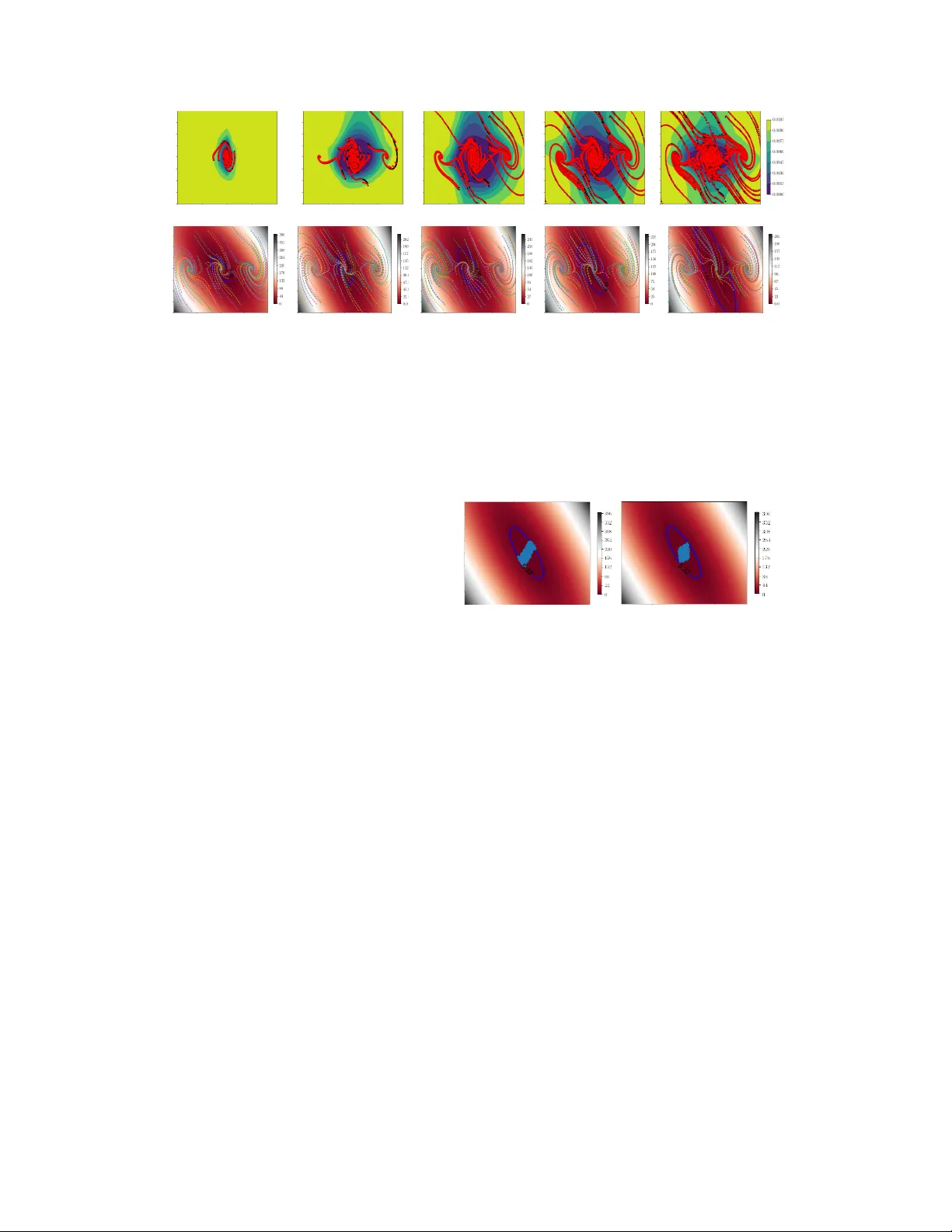
Safe Interactiv e Model-Based Lear ning Marco Gallieri ∗ Seyed Sina Mirraza vi Salehian Nihat Engin T oklu Alessio Quaglino Jonathan Masci Jan K outník Faustino Gomez NN AISENSE, Lugano, Switzerland - Austin, T exas {marco,sina,engin,alessio,jon,jan,tino}@nnaisense.com Abstract Control applications present hard operational constraints. A violation of these can result in unsafe behaviour . This paper introduces Safe Interacti ve Model Based Learning (SiMBL), a frame work to refine an existing controller and a system model while operating on the real en vironment. SiMBL is composed of the follo wing trainable components: a L yapuno v function, which determines a safe set; a safe control polic y; and a Bayesian RNN forward model. A min-max control framework, based on alternate minimisation and backpropagation through the forward model, is used for the of fline computation of the controller and the safe set. Safety is formally verified a-posteriori with a probabilistic method that utilizes the Noise Contrastiv e Priors (NPC) idea to b uild a Bayesian RNN forward model with an additi ve state uncertainty estimate which is large outside the training data distrib ution. Iterati ve refinement of the model and the safe set is achiev ed thanks to a no vel loss that conditions the uncertainty estimates of the ne w model to be close to the current one. The learned safe set and model can also be used for safe exploration, i.e., to collect data within the safe in variant set, for which a simple one-step MPC is proposed. The single components are tested on the simulation of an in v erted pendulum with limited torque and stability region, sho wing that iterati vely adding more data can improv e the model, the controller and the size of the safe region. 1 A pproach rationale Safe Interactiv e Model-Based Learning (SiMBL) aims to control a deterministic dynamical system: x ( t + 1) = x ( t ) + dt f ( x ( t ) , u ( t )) , y ( t ) = x ( t ) , (1) where x is the state and y are the measurements, in this case assumed equi valent. The system (1) is sampled with a known constant time dt and it is subject to closed and bounded, possibly non-con ve x, operational constraints on the state and input: x ( t ) ∈ X ⊆ R n x , u ( t ) ∈ U ⊂ R n u , ∀ t > 0 . (2) The stability of (1) is studied using discrete time systems analysis. In particular , tools from discrete- time contr ol L yapunov functions (Blanchini & Miani, 2007; Khalil, 2014) will be used to compute policies that can keep the system safe . Safety . In this work, safety is defined as the capability of a system to remain within a subset X s ⊆ X of the operational constraints and to return asymptotically to the equilibrium state from anywhere in X s . A feedback control policy , u = K ( x ) ∈ U , is certified as safe if it can pro vide safety with high pr obability . In this work, safety is verified with a statistical method that extends Bobiti (2017). ∗ Corresponding author . Preprint. Under revie w . Safely collectdata Learnmodel Learnsafety conditions Forward mod el Dataset Safety condition Initial controller Iteration == 0 Figure 1: Safe interactive Model-Based Learning (SiMBL) rationale. Approach is centered around an uncertain RNN forward model for which we compute a safe set and a control policy using principles from robust control. This allo ws for safe e xploration though MPC and iterativ e refinement of the model and the safe set. An initial safe polic y is assumed known. Safe learning. The proposed framework aims at learning a policy , K ( x ) , and L ya- punov function, V ( x ) , by means of simu- lated trajectories from an uncertain forward model and an initial polic y K 0 , used to col- lect data. The model, the policy , and the L yapunov function are iteratively refined while safely collecting more data through a Safe Model Predictive Contr oller (Safe- MPC). Figure 1 illustrates the approach. Summary of contrib ution. This w ork presents the algorithms for: 1) Iterativ ely learning a nov el Bayesian RNN model with a large posterior over unseen states and in- puts; 2) Learning a safe set and the associ- ated controller with neural networks from the model trajectories; 3) Safe e xploration with MPC. For 1) and 2), we propose to re- tain the model from scratch using a consistency prior to include knowledge of the pre vious uncertainty and then to recompute the safe set. The safe set increase as more data becomes av ailable and the safety of the exploration strategy are demonstrated on an inv erted pendulum simulation with limited control torque and stability region. Their final integration for continuous model and controller refinement with data from safe exploration (see Figure 1) is left for future work. 2 The Bayesian r ecurrent f orward model A discrete-time stochastic forward model of system (1) is formulated as a Bayesian RNN. A gre y-box approach is used, where a vailable prior kno wledge is integrated into the netw ork in a dif ferentiable way (for instance, the known relation between an observ ation and its deriv ativ e). The model provides an estimate of the next states distrib ution that is large (up to a defined v alue) where there is no av ailable data. This is inspired by recent work on Noise Contrasti ve Priors (NCP) (Hafner et al., 2018b). W e e xtend the NCP approach to RNNs, and propose the Noise Contrasti ve Prior Bayesian RNN (NCP-BRNN), with full state information, which follows the discrete-time update: ˆ x ( t + 1) = ˆ x ( t ) + dt d ˆ x ( t ) , d ˆ x ( t ) = µ ( ˆ x ( t ) , u ( t ); θ µ ) + ˆ w ( t ) , (3) ˆ w ( t ) ∼ q ( ˆ x ( t ) , u ( t ); θ Σ ) , q ( ˆ x ( t ) , u ( t ); θ Σ ) = N (0 , Σ ( ˆ x ( t ) , u ( t ); θ Σ )) , (4) ˆ y ( t ) ∼ N  ˆ x ( t ) , σ 2 y  , ˆ x (0) ∼ N ( x (0) , σ 2 y ) , (5) Σ( · ) = σ w sigm (Σ net ( · )) , µ ( · ) = GreyBox net ( · ) , (6) where ˆ x ( t ) , ˆ y ( t ) denote the state and measurement estimated from the model at time t , and d ˆ x ( t ) is drawn from the distrib ution model, where µ and Σ are computed from neural networks, sharing some initial layers. In particular , µ combines an MLP with some physics prior while the final activ ation of Σ is a sigmoid which is then scaled by the hyperparameter σ w , namely , a finite maximum v ariance. The next state distrib ution depends on the current state estimate ˆ x , the input u , and a set of unknown constant parameters θ , which are to be learned from the data. The estimated state ˆ x ( t ) is for simplicity assumed to have the same physical meaning of the true system state x ( t ) . The system state is measured with a Gaussian uncertainty with standard de viation σ y , which is also learned from data. During the control, the measurement noise is assumed to be negligible ( σ y ≈ 0 ). Therefore, the control algorithms will need to be robust with respect to the model uncertainty . Extensions to partial state information and output noise robust control are also possible b ut are left for future work. T owards reliable uncertainty estimates with RNNs The fundamental assumption for model- based safe learning algorithm is that the model predictions contain the actual system state transitions with high probability (Berkenkamp et al., 2017). This is difficult to meet in practice for most neural network models. T o mitigate this risk, we train our Bayesian RNNs on sequences and include a Noise-Contrastiv e Prior (NCP) term (Hafner et al., 2018b). In the present work, the uncertainty is modelled as a point-wise Gaussian with mean and standard deviation that depend on the current state 2 as well as on the input. The learned 1-step standard deviation, Σ , is assumed to be a diagonal matrix. This assumption is limiting b ut it is common in v ariational neural networks for practicality reasons (Zhao et al., 2017; Chen et al., 2016). The NPC concept is illustrated in Figure 2. More complex uncertainty representations will be considered in future works. The cost function used to train the model is: L ( θ µ , θ Σ ) = − 1 T T X t =0 E p train ( x (0) ,u ( t ))  E q ( ˆ x ( t ) ,u ( t ); θ Σ ) [ln p ( ˆ y ( t ) | y ( t ) , u ( t ); θ µ ; θ Σ )]  + D KL  q ( ˜ x ( t ) , ˜ u ( t ); θ Σ ) || N (0 , σ 2 w )  + E p train ( x (0) ,u ( t ))  ReLU  Σ ( ˆ x ( t ) , u ( t ); θ Σ ) − Σ  ˆ x ( t ) , u ( t ); θ Σ prev  (7) where the first term is the expected negati ve log likelihood ov er the uncertainty distrib ution, ev aluated ov er the training data. The second term is the KL-di vergence which is ev aluated in closed-form ov er predictions ˜ x generated from a set of background initial states and input sequences, ˆ x (0) and ˆ u ( t ) . These are sampled from a uniform distribution for the first model and then, once a previous model is av ailable and new data is collected, they are obtained using rejection sampling with PyMC (Salvatier et al., 2016) with acceptance condition: Σ( ˜ x (0) , ˜ u ( t ); θ Σ prev ) ≥ 0 . 5 σ w . If a previous model is av ailable, then the final term is used which is an uncertainty consistency prior which forces the uncertainty estimates over the training data to not increase with respect to the previous model. The loss (7) is optimised using stochastic backpropagation through truncated sequences. In order to hav e further consistency between model updates, it a previous model is av ailable, we train from scratch but stop optimising once the final loss of the pre vious model is reached. Figure 2: V ariational neural net- works with Noise Contrastive Priors (NCP). Predicting sine-wa ve data (red- black) with confidence bounds (blue area) using NAIS-Net (Ciccone et al., 2018) and NCP (Hafner et al., 2018b). 3 The rob ust control problem W e approximate a chance-constrained stochastic control problem with a min-max robust control problem over a con ve x uncertainty set. This non-conv ex min-max control problem is then also approximated by computing the loss only at the v ertices of the uncertainty set. T o compensate for this approximation, (inspired by v ariational inference) the centre of the set is sampled from the uncertainty distri- bution itself (Figure 3). The procedure is detailed below . L yapunov-Net. The considered L yapunov function is: V ( x ) = x T  I + V net ( x ) T V net ( x )  x + ψ ( x ) , (8) where V net ( x ) is a feedforward network that produces a n V × n x matrix, where n V and  > 0 are hyperparameters. The network parameters have to be trained and they are omitted from the notation. The term ψ ( x ) ≥ 0 represents the prior knowledge of the state constraints. In this work we use: ψ ( x ) = ReLU ( φ ( x ) − 1) , (9) where φ ( x ) ≥ 0 is the Minko wski functional 2 of a user-defined usual r e gion of operation , namely: X φ = { x ∈ X : φ ( x ) ≤ 1 } . (10) Possible choices for the Minko wski functional include quadratic functions, norms or semi-norms (Blanchini & Miani, 2007; Horn & Johnson, 2012). Since V ( x ) must be positiv e definite, the hyperparameter  > 0 is introduced 3 . While other forms are possible as in Blanchini & Miani (2007), with (8) the activ ation function does not need to be in vertible. The study of the generality of the proposed function is left for future consideration. 2 Minko wski functionals measure the distance from the set center and they are positi ve definite. 3 The trainable part of the function V ( x ) is chosen to be piece-wise quadratic but this is not the only possible choice. In fact one can use an y positi ve definite and radially unbounded function. For the same problem multiple L yapunov functions can exist. See also Blanchini & Miani (2007). 3 Safe set definition. Denote the candidate safe level set of V as: X s = { x ⊆ X : V ( x ) ≤ l s } , (11) where l s is the safe lev el. If, for x ∈ X s , the function V ( x ) satisfies the L yapunov inequality ov er the system closed-loop trajectory with a control policy K , namely , u ( t ) = K ( x ( t )) ⇒ V ( x ( t + 1)) − V ( x ( t )) ≤ 0 , ∀ x ( t ) ∈ X s , (12) then set X s is safe , i.e., it satisfies the conditions of positive-in variance (Blanchini & Miani, 2007; K errigan, 2000). Note that the polic y K ( x ) can be either a neural network or a model-based controller, for instance a Linear Quadratic Regulator (LQR, see Kalman (2001)) or a Model Predicti ve Controller (MPC, see Maciejowski (2000); Ra wlings & Mayne (2009); Kouv aritakis & Cannon (2015); Rakovi ´ c & Levine (2019)). A stronger condition to eq. (12) is often used in the context of optimal control: u ( t ) = K ( x ( t )) ⇒ V ( x ( t + 1)) − V ( x ( t )) ≤ − ` ( x ( t ) , u ( t )) , ∀ x ( t ) ∈ X s (13) where ` ( x ( t ) , u ( t )) is a positiv e semi-definite stage loss. In this paper, we focus on training policies with the quadratic loss used in LQR and MPC, where the origin is the target equilibrium, namely: ` ( x, u ) = x T Qx + u T Ru, Q  0 , R  0 . (14) From chance constrained to min-max control Consider the problem of finding a controller K and a function V such that u ( t ) = K ( x ( t )) and: P  V ( ˆ x ( t + 1)) − V ( x ( t )) ≤ − ` ( x ( t ) , u ( u ))  ≥ 1 −  p , (15) where P represents a probability and 0 <  p << 1 . This is a c hance-constrained non-con vex optimal control problem (Kouv aritakis & Cannon, 2015). W e truncate the distributions and approximate (15): max ˆ x ( t +1) ∈ W ( x ( t ) ,u ( t ) ,θ )  V ( ˆ x ( t + 1))  − V ( x ( t )) ≤ − ` ( x ( t ) , K ( x ( t ))) , (16) which is deterministic. A strategy to jointly learn ( V , K ) fulfilling (16) is presented ne xt. 4 Learning the contr oller and the safe set W e wish to build a controller K , a function V , and a safe le vel l s gi ven the state transition probability model, ( µ, Σ) , such that the condition in (13) is satisfied with high probability for the ph ysical system generating the data. Denote the one-step prediction from the model in (3), in closed loop with K , as: ˆ x + = x + dt d ˆ x, with, u = K ( x ) , where ˆ x + represents the next state prediction and the time inde x t is omitted. Appr oximating the high-confidence prediction set. A polytopic approximation of a high confi- dence r e gion of the estimated uncertain set ˆ x + ∈ W ( x, u, θ ) is obtained from the parameters of Σ and used for training ( V , K ) . In this work, the uncertain set is taken as a hyper-diamond centered at x , scaled by the (diagonal) standard deviation matrix, Σ : W 1 ( x, u, θ ) =  x + : x + = x + dt d ˆ x,   (Σ( x, u ; θ Σ )) − 1 ˆ w   1 ≤ ¯ σ  , (17) where ¯ σ > 0 is a hyper -parameter . This choice of set is inspired by the Unscented Kalman filter (W an & V an Der Merwe, 2000). Since Σ is diagonal, the vertices are gi ven by the columns of the matrix resulting from multiplying Σ with a mask M such that: vert [ W ( x, u, θ )] = cols [Σ( x, u ; θ Σ ) M ] , M = ¯ σ [ I , − I ] . (18) Learning the safe set. Assume that a controller K is giv en. Then, we wish to learn a V of the from of (8), such that the corresponding safe set X s is as big as possible, ideally as big as the state constraints X . In order to do so, the parameters of V net are trained using a grid of initial states, a forward model to simulate the next state under the policy K , and an appropriate cost function. The cost for V net and l s is inspired by (Richards et al., 2018). It consists of a combination of two objectiv es: the first one penalises the deviation from the L yapunov stability condition; the second 4 one is a classification penalty that separates the stable points from the unstable ones by means of the decision boundary , V ( x ) = l s . The combined robust L yapunov function cost is: min V net , l s E [ x ( t ) ∈ X gr id ]  J ( x ( t ))  , (19) J ( x ) = I X s ( x ) J s ( x ) + sign  ∇ V ( x )  [ l s − V ( x )] , (20) I X s ( x ) = 0 . 5 ( sign [ l s − V ( x )] + 1) , J s ( x ) = 1 ρV ( x ) ReLU [ ∇ V ( x )] , (21) ∇ V ( x ) = max ˆ x + ∈ W ( x,K ( x ) ,θ )  V  ˆ x +   − V ( x ) + ` ( x, K ( x )) , (22) where ρ > 0 trades of f stability for volume. The robust L yapunov decrease in (22) is ev aluated by using sampling to account for uncertainty over the confidence interv al W . Sampling of the set centre is performed as opposite of setting W = W 1 , which didn’t seem to produce valid results. Let us omit θ for ease of notation. W e substitute ∇ V ( x ) with E W  ∇ V ( x )  , which we define as: E ˆ w ∼N (0 , Σ( x,K ( x )))  max ˆ x + ∈ W 1 ( x,K ( x ) ,θ )+ ˆ w dt  V  ˆ x +    − V ( x ) + ` ( x, K ( x )) , (23) Equations (22) and (23) require a maximisation of the non-con ve x function V ( x ) ov er the con vex set W . For the considered case, a sampling technique or another optimisation (similar to adversarial learning) could be used for a better approximation of the max operator . The maximum over W is instead approximated by the maximum ov er its vertices: ∇ V ( x ) ≈ max ˆ x + ∈ vert [ W 1 ( x,K ( x ) ,θ )]+ ˆ w dt  V  ˆ x +   − V ( x ) + ` ( x, K ( x )) . (24) This consists of a simple enumeration followed by a max over tensors that can be easily handled. Finally , during training (23) is implemented in a v ariational inference fashion by ev aluating (24) at each epoch over a dif ferent sample of ˆ w . This entails a variational posterior ov er the center of the uncertainty interval. The approach is depicted in Figure 3. The proposed cost is inspired by Richards et al. (2018), with the difference that here there is no need for labelling the states as safe by means of a multi-step simulation. Moreover , in this work we train the L yapunov function and controller together , while in (Richards et al., 2018) the latter w as giv en. Learning the safe policy . W e alternate the minimisation of the L yapunov loss (19) and the solution of the variational r obust contr ol problem : min u = K ( x ) E [ x ∈ X gr id ] [ I X s ( x ) L c ( x, u )] , s.t.: K (0) = 0 , (25) L c ( x, u ) = ` ( x, u )+ E W  max ˆ x + ∈ W ( x,u,θ )  V ( ˆ x + ) − γ log( l s − V ( ˆ x + ))   , (26) V ( x ) W 1 Σ 1 Figure 3: Appr oximating the non- con vex maximisation. Centre of the uncertain set is sampled and L yapunov function is ev aluated at its vertices. subject to the forward model (3). In this work, (25) is solved using backpropagation through the policy , the model and V . The safety constraint, ˆ x + ∈ X s , namely , V ( ˆ x + ) ≤ l s is relaxed through a log-barrier (Boyd & V andenberghe, 2004). If a neural policy K ( x ) solves (25) and satisfies the safety constraint, ∀ x ∈ X s , then it is a candidate robust controller for keeping the system within the safe set X s . Note that the expectation in (26) is once again treated as a v ariational approximation of the expectation ov er the center of the uncertainty interval. Obtaining an exact solution to the control problem for all points is computationally impractical. In order to provide statistical guarantees of safety , probabilistic verification is used after V and K hav e been trained. This refines the safe lev el set l s and, if successful, provides a probabilistic safety certificate. If the verification is unsuccessful, then the learned ( X s , K ) are not safe. The data collection continues with the previous safe controller until suitable V , l s , and K are found. Note that the number of training points used for the safe set and controller is in general lower than the ones used for verification. The alternate learning procedure for X s and K is summarised in Algorithm 1. The use of 1-step predictions makes the procedure highly scalable through parallelisation on GPU. 5 Algorithm 1: Alternate descent for safe set In: K 0 , X grid , θ µ , θ Σ , σ w ≥ 0 , ¯ σ > 0 ,  > 0 Out: ( V net , l s , K ) for i = 0 ...N do for j = 0 ...N v do ( V net , l s ) ← Adam step on (20) for j = 0 ...N k do K ← Adam step on (25) Probabilistic safety v erification. A probabilistic verification is used to numerically prov e the phys- ical system stability with high probability . The re- sulting certificate is of the form (15), where the  P decreases with increasing number of samples. Fol- lowing the work of Bobiti (2017), the simulation is ev aluated at a large set of points within the esti- mated safe set X s . Monte Carlo rejection sampling is performed with PyMC (Salvatier et al., 2016). In practical applications, several factors limit the con ver gence of the trajectory to a neighborhood of the target (the ultimate bound , Blanchini & Miani (2007)). For instance, the polic y structural bias, discount factors in RL methods or persistent uncertainty in the model, the state estimates, and the physical system itself. Therefore, we extended the verification algorithm of (Bobiti, 2017) to estimate the ultimate bound as well as the in v ariant set, as outlined in Algorithm 2. Giv en a maximum and minimum le vel, l l , l u , we first sample initial states uniformly within these two le vels and check for a robust decrease of V ov er the ne xt state distribution. If this is verified, then we sample uniformly from inside the minimum lev el set l l (where V may not decrease) and check that V does not exceed the maximum lev el l u ov er the next state distribution. The distribution is ev aluated by means of uniform samples of w , independent of the current state, within ( − ¯ σ , ¯ σ ) . These are then scaled using Σ from the model. W e search for l l , l u with a step δ . Algorithm 2: Probabilistic safety verification In: N , V , K , θ µ , θ Σ , σ w ≥ 0 , ¯ σ > 0 , δ > 0 Out: ( SAFE , l u , l l ) SAFE ← False for l u = 1 , 1 − δ, 1 − 2 δ, ..., 0 do for l l = 0 , δ, 2 δ, ..., l u do draw N uniform x -samples s.t.: l l l s ≤ V ( x ) ≤ l u l s draw N w -samples from U ( − ¯ σ , ¯ σ ) if V ( ˆ x + ) − V ( x ) ≤ 0 , ∀ x, ∀ w then draw N uniform x -samples s.t.: V ( x ) ≤ l l l s if V ( ˆ x + ) ≤ l u l s , ∀ x, ∀ w then SAFE ← True retur n SAFE, l u , l l V erification failed. Note that, in Algorithm 2, the uncertainty of the surrogate model is taken into account by sampling a single uncertainty realisation for the entire set of initial states. The val- ues of w will be then scaled using Σ in the forward model. This step is computation- ally conv enient but breaks the assumption that variables are dra wn from a uniform dis- tribution. W e leave this to future work. In this paper , independent Gaussian uncertainty models are used and stability is verified di- rectly on the en vironment. Note that prob- abilistic verification is e xpensi ve b ut neces- sary , as pathological cases could result in the training loss (19) for the safe set could con ver ging to a local minima with a very small set. If this is the case then usually the forward model is not accurate enough or the uncertainty hyperparameter σ w is too large. Note that Algorithm 2 is highly parallelizable. 5 Safe exploration Once a verified safe set is found the en vironment can be controlled by means of a 1-step MPC with probabilistic stability (see Appendix). Consider the constraint V ( x ) ≤ l ? s = l u l s , where V and l s come from Algorithm 1 and l u from Algorithm 2. The Safe-MPC exploration strategy follo ws: Safe-MPC for exploration. For collecting ne w data, solve the follo wing MPC problem: u ? = arg min u ∈ U  β ` ( x, u ) − α ` expl ( x, u ) + max ˆ x + ∈ W ( x,u,θ )  β V ( ˆ x + ) − γ log( l ? s − V ( ˆ x + ))   , (27) where α ≤ γ is the explor ation hyperparameter , β ∈ [0 , 1] is the r e gulation or exploitation parameter and ` expl ( x, u ) is the info-gain from the model, similar to (Hafner et al., 2018b): ` expl ( x, u ) = X i =1 ,...,N x (Σ ii ( x, u, p, θ )) 2 N x σ 2 y ii . (28) The full deriv ation of the problem and a probabilistic safety result are discussed in Appendix. 6 Alternate min-max optimization. Problem (27) is approximated using alternate descent. In particular , the maximization in the loss function over the uncertain future state ˆ x + with respect to ˆ w , giv en the current control candidate u , is alternated with the minimization with respect to u , giv en the current candidate ˆ x + . Adam (Kingma & Ba, 2014) is used for both steps. 6 In verted pendulum example The approach is demonstrated on an in verted pendulum, where the input is the angular torque and the states/outputs are the angular position and velocity of the pendulum. The aim is to collect data safely around the unstable equilibrium point (the origin). The system has a torque constraint that limits the controllable region. In particular , if the initial angle is greater than 60 degrees, then the torque is not sufficient to swing up the pendulum. In order to compare to the LQR, we choose a linear policy with a tanh activ ation, meeting the torque constraints while preserving differentiability . Safe set with known en vironment, comparison to LQR. W e first test the safe-net algorithm on the nominal pendulum model and compare the policy and the safe set with those from a standard LQR policy . Figure 4 shows the safe set at dif ferent stages of the algorithm, approaching the LQR. i = 1 K = [ − 10 , − 0 . 05] i = 30 K = [ − 9 . 24 , − 1 . 56] i = 50 K = [ − 8 . 49 , − 2 . 25] i = 60 K = [ − 8 . 1 , − 2 . 7] LQR K = [ − 7 . 26 , − 2 . 55] Figure 4: In verted Pendulum. Safe set and controller with proposed method for known envi- ronment model. Initial set ( i = 0 ) is based on a unit circle plus the constraint | α | ≤ 0 . 3 . Contours sho w the function le vels. Control gain gets closer to the LQR solution as iterations progress until circa i = 50 , where the minimum of the L yapunov loss (19) is achiev ed. The set and controller at iteration 50 are closest to the LQR solution, which is optimal around the equilibrium in the unconstrained case. In order to maximise the chances of verification the optimal parameters are selected with a early stopping, namely when the L yapunov loss reaches its minimum, resulting in K = [ − 8 . 52 , − 2 . 2] . Safe set with Bay esian model. In order to test the proposed algorithms, the forw ard model is fitted on sequences of length 10 for an increasing amount of data points ( 10 k to 100 k ). Data is collected in closed loop with the initial controller , K 0 = [ − 10 , 0] , with dif ferent initial states. In particular , we perturb the initial state and control values with a random noise with standard de viations starting from, respecti vely , 0 . 1 and 0 . 01 and doubling each 10 k points. The only prior used is that the velocity is the deri vati ve of the angular position (normalized to 2 π and π ). The uncertainty bound w as fixed to σ w = 0 . 01 . The architecture was cross-v alidated from 60 k datapoints with a 70 - 30 split. The model with the best validation predictions as well as the lar gest safe set was used to generate the results in Figure 6. (a) en vironment (b) NCP-BRNN ( 80 k points). Figure 5: In verted pendulum v erification . Nominal and robust safe sets are v erified on the pendulum sim- ulation using 5 k samples. W e search for the largest stability region and the smallest ultimate bound of the solution. If a simulation is not av ailable, then a two-le vel sampling on BRNN is performed. The results demonstrate that the size of the safe set can improve with more data, pro- vided that the model uncertainty decreases and the predictions hav e comparable accu- racy . This motiv ates for exploration. V erification on the envir onment. The candidate L yapunov function, safe le vel set, and robust control policy are formally verified through probabilistic sampling of the system state, according to Algorithm 2, where the simulation is used directly . The results for 5 k samples are sho wn in Figure 5. In particular , the computed level sets verify at the first attempt and no further search for sub-lev els or ultimate bounds is needed. 7 10 k points 30 k points 50 k points 70 k points 90 k points 10 k points 30 k points 50 k points 80 k points en vironment Figure 6: In verted pendulum safe set with Bayesian model. Surrogates are obtained with in- creasing amount of data. The initial state and input perturbation from the safe policy are drawn from Gaussians with standard deviation that doubles each 10 k points. T op : Mean predictions and uncertainty contours for the NCP-BRNN model. After 90 k points no further improvement is noticed. Bottom : Comparison of safe sets with surrogates and en vironment. Reducing the model uncertainty while maintaining a similar prediction accuracy leads to an increase in the safe set. After 90 k points no further benefits are noticed on the set which is consistent with the uncertainty estimates. Semi-random exploration 50 trials of 1 k steps vol = 0 . 06 Safe-MPC exploration 1 trial of 50 k steps vol = 0 . 04 Figure 7: Safe exploration . Comparison of a naive semi-random exploration strategy with the proposed Safe-MPC for exploration. The proposed algorithm has an efficient space co verage with safety guarantees. Safe exploration. Safe exploration is per - formed using the min-max approach in Sec- tion 5. For comparison, a semi-random ex- ploration strategy is also used: if inside the safe set, the action magnitude is set to maxi- mum torque and its sign is giv en by a random uniform variable once V ( x ) ≥ 0 . 99 l s , then the safe policy K is used. This does not pro- vide any formal guarantees of safety as the value of V ( x ) could exceed the safe lev el, especially for very fast systems and large in- put signals. This is repeated for se veral trials in order to estimate the maximum reachable set within the safe set. The results are shown in Figure 7, where the semi-random strategy is used as a baseline and is compared to a single trial of the proposed safe-exploration algorithm. The area covered by our algorithm in a single trial of 50 k steps is about 67% of that of the semi-random baseline ov er 50 trials of 1 k steps. Extending the length of the trials did not significantly improve the baseline results. Despite being more conservati ve, our algorithm continues to explore safely indefinitely . 7 Conclusions Preliminary results sho w that the SiMBL produces a L yapunov function and a safe set using neural networks that are comparable with that of standard optimal control (LQR) and can account for state-dependant additiv e model uncertainty . A Bayesian RNN surrogate with NCP was proposed and trained for an in verted pendulum simulation. An alternate descent method was presented to jointly learn a L yapunov function, a safe le vel set, and a stabilising control polic y for the surrogate model with back-propagation. W e demonstrated that adding data-points to the training set can increase the safe-set size provided that the model improves and its uncertainty decreases. T o this end, an uncertainty prior from the previous model was added to the framework. The safe set was then formally verified through a nov el probabilistic algorithm for ultimate bounds and used for safe data collection (exploration). A one-step safe MPC w as proposed where the L yapunov function pro vides the terminal cost and constraint to mimic an infinite horizon with high probability of recursive feasibility . Results show that the proposed safe-exploration strategy has better coverage than a naive policy which switches between random inputs and the safe policy . 8 References Akametalu, A. K., Fisac, J. F ., Gillula, J. H., Kaynama, S., Zeilinger , M. N., & T omlin, C. J. (2014). Reachability-based safe learning with gaussian processes. In 53rd IEEE Confer ence on Decision and Contr ol . IEEE. URL https://doi.org/10.1109/cdc.2014.7039601 Bemporad, A., Borrelli, F ., & Morari, M. (2003). Min-max control of constrained uncertain discrete- time linear systems. Automatic Contr ol, IEEE T ransactions on , 48 , 1600 – 1606. Ben-T al, A., Ghaoui, L. E., & Nemirovski, A. (2009). Robust Optimization (Princeton Series in Applied Mathematics) . Princeton Univ ersity Press. Berkenkamp, F ., T urchetta, M., Schoellig, A. P ., & Krause, A. (2017). Safe Model-based Reinforce- ment Learning with Stability Guarantees. arXiv:1705.08551 [cs, stat] . ArXiv: 1705.08551. URL Blanchini, F ., & Miani, S. (2007). Set-Theoretic Methods in Control (Systems & Contr ol: F oundations & Applications) . Birkhäuser . Bobiti, R., & Lazar , M. (2016). Sampling-based verification of L yapunov’ s inequality for piece wise continuous nonlinear systems. arXiv:1609.00302 [cs] . ArXiv: 1609.00302. URL Bobiti, R. V . (2017). Sampling driven stability domains computation and pr edictive control of constrained nonlinear systems . Ph.D. thesis. URL https://pure.tue.nl/ws/files/78458403/20171025_Bobiti.pdf Borrelli, F ., Bemporad, A., & Morari, M. (2017). Predictive Contr ol for Linear and Hybrid Systems . Cambridge Univ ersity Press. Boyd, S., & V andenber ghe, L. (2004). Con vex Optimization . New Y ork, NY , USA: Cambridge Univ ersity Press. Camacho, E. F ., & Bordons, C. (2007). Model Predictive contr ol . Springer London. Carron, A., Arcari, E., W ermelinger , M., Hewing, L., Hutter , M., & Zeilinger , M. N. (2019). Data- driv en model predicti ve control for trajectory tracking with a robotic arm. URL http://hdl.handle.net/20.500.11850/363021 Chen, X., Kingma, D. P ., Salimans, T ., Duan, Y ., Dhariwal, P ., Schulman, J., Sutske ver , I., & Abbeel, P . (2016). V ariational Lossy Autoencoder. arXiv:1611.02731 [cs, stat] . ArXiv: 1611.02731. URL Cheng, R., Orosz, G., Murray , R. M., & Burdick, J. W . (2019). End-to-End Safe Reinforcement Learn- ing through Barrier Functions for Safety-Critical Continuous Control T asks. arXiv:1903.08792 [cs, stat] . ArXiv: 1903.08792. URL Chow , Y ., Nachum, O., Duenez-Guzman, E., & Ghav amzadeh, M. (2018). A L yapunov-based Approach to Safe Reinforcement Learning. arXiv:1805.07708 [cs, stat] . ArXiv: 1805.07708. URL Chow , Y ., Nachum, O., Faust, A., Duenez-Guzman, E., & Ghav amzadeh, M. (2019). L yapunov- based Safe Policy Optimization for Continuous Control. arXiv:1901.10031 [cs, stat] . ArXiv: 1901.10031. URL Chua, K., Calandra, R., McAllister, R., & Levine, S. (2018). Deep Reinforcement Learning in a Handful of T rials using Probabilistic Dynamics Models. arXiv:1805.12114 [cs, stat] . ArXi v: 1805.12114. URL Ciccone, M., Gallieri, M., Masci, J., Osendorfer, C., & Gomez, F . (2018). Nais-net: Stable deep networks from non-autonomous dif ferential equations. In NeurIPS . 9 Deisenroth, M., & Rasmussen, C. (2011). Pilco: A model-based and data-efficient approach to polic y search. In Proceedings of the 28th International Confer ence on Machine Learning , ICML 2011 , (pp. 465–472). Omnipress. Deisenroth, M. P ., Fox, D., & Rasmussen, C. E. (2015). Gaussian Processes for Data-Efficient Learning in Robotics and Control. IEEE T ransactions on P attern Analysis and Machine Intelligence , 37 (2), 408–423. ArXiv: 1502.02860. URL Depewe g, S., Hernández-Lobato, J. M., Doshi-V elez, F ., & Udluft, S. (2016). Learning and Policy Search in Stochastic Dynamical Systems with Bayesian Neural Networks. arXiv:1605.07127 [cs, stat] . ArXiv: 1605.07127. URL Frigola, R., Chen, Y ., & Rasmussen, C. E. (2014). V ariational gaussian process state-space models. In NIPS . Gal, Y ., McAllister , R., & Rasmussen, C. E. (2016). Improving PILCO with Bayesian neural network dynamics models. In Data-Efficient Mac hine Learning workshop, ICML . Gallieri, M. (2016). Lasso-MPC – Pr edictive Contr ol with ` 1 -Re gularised Least Squar es . Springer International Publishing. URL https://doi.org/10.1007/978- 3- 319- 27963- 3 Gros, S., & Zanon, M. (2019). T ow ards Safe Reinforcement Learning Using NMPC and Policy Gradients: Part II - Deterministic Case. arXiv:1906.04034 [cs] . ArXiv: 1906.04034. URL Hafner , D., Lillicrap, T ., Fischer , I., V illegas, R., Ha, D., Lee, H., & Da vidson, J. (2018a). Learning Latent Dynamics for Planning from Pixels. arXiv:1811.04551 [cs, stat] . ArXiv: 1811.04551. URL Hafner , D., T ran, D., Irpan, A., Lillicrap, T ., & Davidson, J. (2018b). Reliable Uncertainty Estimates in Deep Neural Networks using Noise Contrastiv e Priors. arXiv:1807.09289 [cs, stat] . ArXiv: 1807.09289. URL He wing, L., Kabzan, J., & Zeilinger, M. N. (2017). Cautious Model Predicti ve Control using Gaussian Process Regression. arXiv:1705.10702 [cs, math] . ArXiv: 1705.10702. URL Horn, R. A., & Johnson, C. R. (2012). Matrix Analysis . New Y ork, NY , USA: Cambridge University Press, 2nd ed. Kalman, R. (2001). Contribution to the theory of optimal control. Bol. Soc. Mat. Mexicana , 5 . Kerrig an, E. (2000). Robust constraint satisfaction: In variant sets and predicti ve control. T ech. rep. URL http://hdl.handle.net/10044/1/4346 Kerrig an, E. C., & Maciejo wski, J. M. (2004). Feedback min-max model predicti ve control using a single linear program: robust stability and the e xplicit solution. International Journal of Rob ust and Nonlinear Contr ol , 14 (4), 395–413. URL https://doi.org/10.1002/rnc.889 Khalil, H. K. (2014). Nonlinear Contr ol . Pearson. Kingma, D. P ., & Ba, J. (2014). Adam: A Method for Stochastic Optimization. [cs] . ArXiv: 1412.6980. URL K oller , T ., Berkenkamp, F ., T urchetta, M., & Krause, A. (2018). Learning-based Model Predictiv e Control for Safe Exploration and Reinforcement Learning. arXiv:1803.08287 [cs] . ArXiv: 1803.08287. URL 10 K ouv aritakis, B., & Cannon, M. (2015). Model Pr edictive Contr ol: Classical, Robust and Stochastic . Advanced T extbooks in Control and Signal Processing, Springer , London. Kurutach, T ., Clav era, I., Duan, Y ., T amar , A., & Abbeel, P . (2018). Model-Ensemble Trust-Re gion Policy Optimization. arXiv:1802.10592 [cs] . ArXiv: 1802.10592. URL Limon, D., Calliess, J., & Maciejo wski, J. (2017). Learning-based nonlinear model predictiv e control. IF AC-P apersOnLine , 50 (1), 7769–7776. URL https://doi.org/10.1016/j.ifacol.2017.08.1050 Lorenzen, M., Cannon, M., & Allgower , F . (2019). Robust MPC with recursiv e model update. Automatica , 103 , 467–471. URL https://ora.ox.ac.uk/objects/pubs:965898 Lowre y , K., Rajeswaran, A., Kakade, S., T odorov , E., & Mordatch, I. (2018). Plan Online, Learn Of fline: Efficient Learning and Exploration via Model-Based Control. arXiv:1811.01848 [cs, stat] . ArXiv: 1811.01848. URL Maciejowski, J. (2000). Pr edictive Contr ol with Constraints . Prentice Hall. Mayne, D. Q., Ra wlings, J. B., Rao, C. V ., & Scokaert, P . O. M. (2000). Constrained model predicti ve control: Stability and optimality . Papini, M., Battistello, A., Restelli, M., & Battistello, A. (2018). Safely exploring policy gradient. Pozzoli, S. (2019). State Estimation and Recurr ent Neural Networks for Model Pr edictive Contr ol . Politecnico di Milano, MS thesis, supervisors: R. Scattolini, M. Gallieri, E. T erzi, M. Farina. Pozzoli, S., Gallieri, M., & Scattolini, R. (2019). T ustin neural networks: a class of recurrent nets for adaptiv e MPC of mechanical systems. arXiv:1911.01310 [cs, eess] . ArXiv: 1911.01310. URL Raimondo, D., Limon, D., Lazar , M., Magni, L., & Camacho, E. (2009). Min-max model predictiv e control of nonlinear systems: A unifying overvie w on stability . Eur opean Journal of Contr ol , 15 . Rakovi ´ c, S. V ., K ouvaritakis, B., Findeisen, R., & Cannon, M. (2012). Homothetic tube model predictiv e control. Automatica , 48 , 1631–1638. Rakovi ´ c, S. V ., & Levine, W . S. (Eds.) (2019). Handbook of Model Predictive Contr ol . Springer International Publishing. URL https://doi.org/10.1007/978- 3- 319- 77489- 3 Rawlings, J. B., & Mayne, D. Q. (2009). Model Predictive Contr ol Theory and Design . Nob Hill Pub, Llc. Richards, A. G. (2004). Robust Constr ained Model Pr edictive Contr ol , . Ph.D. thesis, MIT . Richards, S. M., Berkenkamp, F ., & Krause, A. (2018). The L yapunov Neural Network: Adaptive Stability Certification for Safe Learning of Dynamical Systems. arXiv:1808.00924 [cs] . ArXiv: 1808.00924. URL Salimans, T ., Ho, J., Chen, X., Sidor , S., & Sutske ver , I. (2017). Evolution strate gies as a scalable alternativ e to reinforcement learning. arXiv pr eprint arXiv:1703.03864 . Salvatier , J., W iecki, T . V ., & Fonnesbeck, C. (2016). Probabilistic programming in python using PyMC3. P eerJ Computer Science , 2 , e55. URL https://doi.org/10.7717/peerj- cs.55 Shyam, P ., Jasko wski, W ., & Gomez, F . (2018). Model-based activ e exploration. CoRR , abs/1810.12162 . URL 11 Stanley , K. O., & Miikkulainen, R. (2002). Evolving neural networks through augmenting topologies. Evolutionary computation , 10 (2), 99–127. T aylor , A. J., Dorobantu, V . D., Le, H. M., Y ue, Y ., & Ames, A. D. (2019). Episodic Learning with Control L yapunov Functions for Uncertain Robotic Systems. arXiv:1903.01577 [cs] . ArXiv: 1903.01577. URL Thananjeyan, B., Balakrishna, A., Rosolia, U., Li, F ., McAllister, R., Gonzalez, J. E., Le vine, S., Borrelli, F ., & Goldberg, K. (2019). Safety Augmented V alue Estimation from Demonstrations (SA VED): Safe Deep Model-Based RL for Sparse Cost Robotic T asks. arXiv:1905.13402 [cs, stat] . ArXiv: 1905.13402. URL V erdier , C. F ., & M. Mazo, J. (2017). Formal Controller Synthesis via Genetic Programming. IF A C- P apersOnLine , 50 (1), 7205–7210. URL https://doi.org/10.1016/j.ifacol.2017.08.1362 V inogradska, J. (2017). Gaussian Processes in Reinforcement Learning: Stability Analysis and Efficient V alue Propagation. URL http://tuprints.ulb.tu- darmstadt.de/7286/1/GPs_in_RL_Stability_ Analysis_and_Efficient_Value_Propagation_Version1.pdf W abersich, K. P ., He wing, L., Carron, A., & Zeilinger, M. N. (2019). Probabilistic model predictive safety certification for learning-based control. arXiv:1906.10417 [cs, eess] . ArXiv: 1906.10417. URL W an, E., & V an Der Merwe, R. (2000). The unscented kalman filter for nonlinear estimation. (pp. 153–158). W illiams, G., W agener , N., Goldfain, B., Drews, P ., Rehg, J. M., Boots, B., & Theodorou, E. A. (2017). Information theoretic MPC for model-based reinforcement learning. In 2017 IEEE International Confer ence on Robotics and Automation (ICRA) . IEEE. URL https://doi.org/10.1109/icra.2017.7989202 Y an, S., Goulart, P ., & Cannon, M. (2018). Stochastic Model Predictiv e Control with Discounted Probabilistic Constraints. ArXiv: 1807.07465. URL Y ang, X., & Maciejo wski, J. (2015a). Risk-sensitiv e model predictiv e control with gaussian process models. IF AC-P apersOnLine , 48 (28), 374–379. URL https://doi.org/10.1016/j.ifacol.2015.12.156 Y ang, X., & Maciejo wski, J. M. (2015b). Fault tolerant control using gaussian processes and model predictiv e control. International Journal of Applied Mathematics and Computer Science , 25 (1), 133–148. URL https://doi.org/10.1515/amcs- 2015- 0010 Zhao, S., Song, J., & Ermon, S. (2017). InfoV AE: Information Maximizing V ariational Autoencoders. arXiv:1706.02262 [cs, stat] . ArXiv: 1706.02262. URL 12 A Robust optimal contr ol for safe lear ning Further detail is provided re garding robust and chance constrained control. Chance-constrained and rob ust control. Consider the problem of finding a controller K and a function V such that u ( t ) = K ( x ( t )) and: P  V ( ˆ x ( t + 1)) − V ( x ( t )) ≤ − ` ( x ( t ) , u ( u ))  ≥ 1 −  p , (29) where ˆ x is given by the forward model (3), P represents a probability and 0 <  p << 1 . This is a chance-constrained control problem (Kouv aritakis & Cannon, 2015; Y an et al., 2018). Since finding K and V that satisfy (29) requires solving a non-con vex and also stochastic optimization, we approximate (29) with a min-max condition over a high-confidence interv al, in the form of a con vex set W ( x ( t ) , u ( t ) , θ ) , as follows: max ˆ x ( t +1) ∈ W ( x ( t ) ,u ( t ) ,θ )  V ( ˆ x ( t + 1))  − V ( x ( t )) ≤ − ` ( x ( t ) , K ( x ( t ))) , (30) This is a robust control problem, which is still non-conv ex b ut deterministic. In the conv ex case, (30) can be satisfied by means of robust optimization (Ben-T al et al., 2009; Ra wlings & Mayne, 2009). By following this consideration, we frame the control problem as a non-con ve x min-max optimization. Links to optimal control and intrinsic robustness. T o link our approach with optimal control and reinforcement learning, note that if the condition in (13) is met with equality , then the controller K and the L yapunov function V satisfy the Bellman equation (Rawlings & Mayne, 2009). Therefore, u = K ( x ) is optimal and V ( x ) is the value-function of the infinite horizon optimal control problem with stage loss ` ( x, u ) . In practice, this condition is not met with exact equality . Nev ertheless, the inequality in (13) guarantees by definition that the system controlled by K ( x ) is asymptotically stable (con ver ges to x = 0 ) and it has a degree of tolerance to uncertainty in the safe set X s (i.e. if the system is locally Lipschitz) (Rawlings & Mayne, 2009). V ice versa, infinite horizon optimal control with the considered cost produces a v alue function which is also a L yapunov function and provides an intrinsic degree of rob ustness (Rawlings & Mayne, 2009). B From r obust MPC to safe exploration Once a robust L yapunov function and in variant set are found, the en vironment can be controlled by means of a one-step MPC with probabilistic safety guarantees. One-step rob ust MPC. Start by considering the following min-max 1-step MPC problem: u ? = arg min u ∈ U  ` ( x, u ) + max ˆ x + ∈ W ( x,u,θ )  V ( ˆ x + )   , (31) s.t. max ˆ x + ∈ W ( x,u,θ )  V ( ˆ x + )  ≤ l s , and to (3) – (42) , giv en x = x ( t ) , with V ( x ) ≤ l s . This is a non-con ve x min-max optimisation problem with hard non-con ve x constraints. Solving (31) is difficult, especially in real-time, but is in general possible if the constraints are feasible. This is true with a probability that depends from the verification procedure, the confidence le vel used in the procedures, as well as the probability of the model being correct. Relaxed problem. Solutions of (31) can be computed in real-time, to a degree of accuracy , by iterativ e conv exification of the problem and the use of fast conv ex solvers. This is described in Appendix. For the purpose of this paper , we will consider the soft-constrained or r elaxed problem: u ? = arg min u ∈ U  ` ( x, u ) + max ˆ x + ∈ W ( x,u,θ )  V ( ˆ x + ) − γ log( l s − V ( ˆ x + ))   , (32) once again subject to (3). It is assumed that a scalar, γ > 0 , exists such that the constraint can be enforced. For the sak e of simplicity , problem (32) will be addressed using backpropagation, at the price of losing real-time guarantees. 13 Safe exploration. For collecting new data, we modify the rob ust MPC problem as follo ws: u ? = arg min u ∈ U  β ` ( x, u ) − α ` expl ( x, u ) + max ˆ x + ∈ W ( x,u,θ )  β V ( ˆ x + ) − γ log( l s − V ( ˆ x + ))   , (33) where α ≤ γ is the explor ation hyperparameter , β ∈ [0 , 1] is the r e gulation or exploitation parameter and ` expl ( x, u ) is the info-gain from the model, similar to (Hafner et al., 2018b): ` expl ( x, u ) = X i =1 ,...,N x (Σ ii ( x, u, p, θ )) 2 N x σ 2 y ii . (34) Probabilistic Safety . W e study the feasibility and stability of the proposed scheme, following the framew ork of Mayne et al. (2000); Rawlings & Mayne (2009). In particular, if the MPC (31) is always feasible , and the terminal cost and terminal set satisfy (15) with probability 1 , then the MPC (31) enjoys some intrinsic r obustness properties. In other words, we should be able to control the physical system and come back to a neighborhood of the initial equilibrium point for any state in X s , the size of this neighborhood depending on the model accuracy . W e assume a perfect solver is used and that the relaxed problems enforce the constraints e xactly for a giv en γ . For the exploration MPC to be safe , we wish to be able to find a u ? ( t ) satisfying the terminal constraint: V ( ˆ x + ( t )) ≤ l s , ∀ t, starting from the stochastic system: ˆ x + ( t ) = x ( t ) + ( µ ( x ( t ) , u ? ( t ) , θ µ ) + w ( t )) dt, w ( t ) ∼ N (0 , Σ( x ( t ) , u ? ( t ) , θ Σ )) . W e aim at a probabilistic result. First, recall that we truncate the distribution of, w , to a high confidence lev el z-score, ¯ σ . Once again, we switch to a set-valued uncertainty representation as it is most con venient and provide a result that depends on the z-score ¯ σ . Assume known the probability of our model to be able to perform one step predictions, gi ven the model M , such that the real state increments are within the gi ven confidence interv al, ¯ σ , and define it as: P ( x ( t + 1) ∈ M ( x ( t )) |M , ¯ σ ) = 1 −  M ( ¯ σ ) . This probability can be estimated and improv ed using cross- validation, for instance by fine-tuning σ w . It can also be increased with ¯ σ after the model training. This can howe ver make the control search more challenging. Finally , since we use probabilistic verification, from (15) we have a probability of the terminal set to be in variant for the model with truncated distributions: P ( R ( X s ) ⊆ X s |M , ¯ σ ) = P ( R ( X s ) ⊆ X s ) = 1 −  p , where R is the one-step reachability set operator (Kerrigan, 2000) computed using the model in closed loop with K . Note that this probability is determined by the number of verification samples (Bobiti, 2017). Safety of the next state is determined by: Theorem 1. Given x ( t ) ∈ X s , the pr obability of (31-33) to be feasible (safe) at the next time step is: P ( x ( t + 1) ∈ X s |M , ¯ σ , x ( t ) ∈ X s ) = (35) P ( x ( t + 1) ∈ M ( x ( t )) |M , ¯ σ ) P ( R ( X s ) ⊆ X s ) = (36) (1 −  M ( ¯ σ ))(1 −  p ) . (37) It must be noticed that, whilst P ( R ( X s ) ⊆ X s ) is constant, the size of X s will generally decrease for increasing ¯ σ as well as σ w . The probability of any state to lead to safety in the next step is gi ven by: Theorem 2. Given x ( t ) , the pr obability of (31-33) to be feasible (safe) at the next step is: P SAFE ( M , ¯ σ ) = P ( x ( t ) ∈ C ( X s )) P ( x ( t + 1) ∈ X s |M , ¯ σ , x ( t ) ∈ X s ) ≥ (38) P ( x ( t ) ∈ X s )(1 −  M ( ¯ σ ))(1 −  p ) , (39) where C denotes the one-step robust controllable set for the model (K errigan, 2000). The size of the safe set is a key factor for a safe system. This depends also on the architecture of V and K as well as on the stage cost matrices Q and R . A stage cost is not explicitly needed for the proposed approach, ho wev er , Q can be beneficial in terms of additional robustness and R serves as a re gularisation for K . 14 C Network ar chitecture f or in verted pendulum Forward Model Recall the NPC-BRNN definition: ˆ x ( t + 1) = ˆ x ( t ) + dt d ˆ x ( t ) , d ˆ x ( t ) = µ ( ˆ x ( t ) , u ( t ); θ µ ) + ˆ w ( t ) , (40) ˆ w ( t ) ∼ q ( ˆ x ( t ) , u ( t ); θ Σ ) , q ( ˆ x ( t ) , u ( t ); θ Σ ) = N (0 , Σ ( ˆ x ( t ) , u ( t ); θ Σ )) , (41) ˆ y ( t ) ∼ N  ˆ x ( t ) , σ 2 y  , ˆ x (0) ∼ N ( x (0) , σ 2 y ) . (42) Partition the state as x = [ x 1 x 2 ] T , where the former represents the angular position and the latter the velocity . They are normalised, respectiv ely , to a range of ± π and ± 2 π . W e consider a µ of the form: µ ( x, u ) =  2 · x 2 f µ ( x, u )  (43) where f µ ( x, u ) is a three-layer feed-forward neural network with 64 hidden units and tanh acti vations in the two hidden layers. The final layer is linear . The first layer of f µ is shared with the standard deviation network, Σ( x, u ) , where it is then follo wed by one further hidden layer of 64 units before the final sigmoid layer . The parameter σ w is set to 0 . 01 . The noise standard deviation, σ y is passed through a softplus layer in order to maintain it positi ve and w as initialised at 0 . 01 by in verting the softplus. W e used 1000 epochs for training, with a learning rate of 1E-4 and an horizon of 10 . The sequences where all of 1000 samples, the number of sequences w as increased by increments of 10 and the batch size adjusted to hav e sequences of length 10 . The target loss was initilisized as − 2 . 94 . W e point out that this architecture is quite general and has been positi vely tested on other applications, for instance a double pendulum or a joint-space robot model, with states partitioned accordingly . L yapunov function The L yapunov net consists of three fully-connected hidden layers with 64 units and tanh acti vations which are then follo wed by a final linear layer with 200 outputs. These are then reshaped into a matrix, V net , of size 100 × 2 and is ev aluated as: V ( x ) = x T sofplus ( α )  I + V net ( x ) T V net ( x )  x + ψ ( x ) , (44) where  > 0 is a hyperparameter and α is a trainable scaling parameter which is passed through a softplus. The introduction of α noticeably improved results. The prior function φ was set to keep | x 1 | ≤ 0 . 3 . W e used 61 outer epochs for training and 10 inner epochs for the updates of V and K , with a with learning rate 1E-3. W e used a uniform grid of 10 k initial stastes as a single batch. Exploration MPC For demonstrati ve purposes we solv ed the Safe-MPC using Adam with 3000 epochs for the minimisation step and SGD with 100 epochs for the maximisation step. The outer loop used 3 iterations. The learning rates were set to, respectiv ely , 0 . 1 and 1E-4. The exploration factor , α , was set to 100 as well as the soft constraint factor , γ . The exploitation factor , β , was set to 1 . D Considerations on model refinement and policies Using neural networks present se veral adv antages ov er other popular inference models: for instance, their scalability to high dimensional and to large amount of data, the ease of including physics-based priors and structure in the architecture and the possibility to learn ov er long sequences. At the same time, NNs require more data than other methods and no offer no formal guarantees. For the guarantees, we hav e considered a-posteriori probabilistic verification. For the larger amount of data, we hav e assumed that an initial controller exists (this is often the case) that can be used to safely collect as much data as we need. Model refinement. A substantial difficulty was encountered while trying to incrementally improve the results of the neural network with increasing amount data. In particular , as more data is collected, larger or more batches must be used. This implies that either the gradient computation or the number of backward passes performed per epoch is dif ferent from the pre vious model training. Consequentely , if a model is retrained entirely from scratch, then the final loss and the network parameters can be substantially different from the ones obtained in the previous trial. This might result in having a larger uncertainty than before in certain regions of the state space. If this is the case, then stabilising the model can become more dif ficult and the resulting safe set might be smaller . W e have observ ed 15 this pathology initially and have mitigated it by employing these particular steps: first, we use a sigmoid layer to effecti vely limit the maximum uncertainty to a known h yperparameter; second, we added a consistency loss that encourages the ne w model to hav e uncertainty smaller than the pre vious one ov er the (ne w) training set; third, we used rejection sampling for the background based on the uncertainty of the pre vious model, so that the NCP does not penalise pr eviously known datapoints; finally , we stop the training loop as soon as the final loss of the pre vious model is exceeded. These ingredients hav e prov en successful in reducing this pathology and, together with having training data with increasing variance, ha ve provided that the uncertainty and safe set improve up to 90 k datapoints. After that, howe ver , adding further datapoints has not improv ed the size of the safe set which has not reached its maximial possible size. W e believe that closing the loop with e xploration could improv e on this result but are also going to in vestigate further alternati ves. Noticeably , Gal et al. (2016) remarked that improving their BNN model w as not simple. They tried for instance to use a forgetting factor which was not successful and concluded that their best solution was to sav e only a fixed number of most recent trials. W e believ e this could not be sufficient for safe learning as the uncertain space needs to be explored. Future work will further address this topic, for instance, by retraining only part of the network, or possibly by exploring combinations of our approach with the ensemble approach used in Shyam et al. (2018). Initial trials of the former seemed encouraging for deterministic models. T raining NNs as robust contr ollers. In this paper , we hav e used a neural network polic y for the computation of the safe controller . This choice was made fundamentally to compare the results with an LQR, which can successfully solve the example. T raining policies with backpropagation is not an easy task in general. For more complex scenarios, we en visage two possible solutions: the first is to use e volutionary strate gies (Stanley & Miikkulainen, 2002; Salimans et al., 2017) or other global optimisation methods to train the policy; the second is to use a robust MPC instead of a policy . Initial trials of the former seemed encouraging. The latter would result in a change of Algorithm 1, where the K would be not learned but just ev aluated point-wise through an MPC solver . Future work is going to in vestig ate these alternativ es. E Related work Robust and Stochastic MPC Robust MPC can be formulated using se veral methods, for instance: min-max optimisation (Bemporad et al., 2003; Kerrigan & Maciejowski, 2004; Raimondo et al., 2009), tube MPC (Rawlings & Mayne, 2009; Rako vi ´ c et al., 2012) or constraints restriction (Richards, 2004) provide rob ust recursive feasibility gi ven a kno wn bounded uncertainty set. In tube MPC as well as in constraints restriction, the nominal cost is optimized while the constraints are restricted according to the uncertainty set estimate. This method can be more conservati ve but it does not require the maximization step. For non-linear systems, computing the required control in v ariant sets is generally challenging. Stochastic MPC approaches the control problem in a probabilistic way , either using expected or probabilistic constraints. For a broad revie w of MPC methods and theory one can refer to Maciejo wski (2000); Camacho & Bordons (2007); Ra wlings & Mayne (2009); K ouv aritakis & Cannon (2015); Gallieri (2016); Borrelli et al. (2017); Rakovi ´ c & Levine (2019). Adaptive MPC Lorenzen et al. (2019) presented an approach based on tube MPC for linear parameter varying systems using set membership estimation. In particular , the constraints and model parameter set estimates are updated in order to guarantee recursiv e feasibility . Pozzoli et al. (2019) used the Unscented Kalman Filter (UKF) to adapt online the last layer of a nov el RNN architecture, the T ustin Net (TN), which was then used to successfully control a double pendulum though MPC. TN is a deterministic RNN which is related to the architecture used in this paper . A comparison of different network architectures, estimation and adaptation heuristics for neural MPC can be found, for instance, in Pozzoli (2019). Stability certification Bobiti & Lazar (2016) proposed a grid-based deterministic verification method which relies on local Lipschitz bounds of the system dynamics. This approach requires knowledge of the model equations and it was extended to black-box simulations (Bobiti, 2017) using a probabilistic approach. W e extend this frame work by means of a check for ultimate boundedness and propose to use it with Bayesian models through uncertainty sampling. 16 MPC for Reinfor cement Learning W illiams et al. (2017) presented an information-theoretical framew ork to solve a non-linear MPC in real-time using a neural network model and performed model-based RL on a race car scale-model with non-con ve x constraints. Gros & Zanon (2019) used policy gradient methods to learn a classic rob ust MPC for linear systems. Safe learning Y ang & Maciejo wski (2015a,b) looked, respecti vely , at using GPs for risk sensitive and fault-tolerant MPC. V inogradska (2017) proposed a quadrature method for computing in variant sets, stabilising and unrolling GP models for use in RL. Berkenkamp et al. (2017) used the deter- ministic verification method of (Bobiti & Lazar, 2016) on GP models and embedded it into an RL framew ork using approximate dynamic programming. The resulting policy has a high probability of safety . Akametalu et al. (2014) studied the reachable sets of GP models and proposed an iterativ e procedure to refine the stabilisable (safe) set as more data is collected. Hewing et al. (2017) re vie wed uncertainty propagation methods and formulated a chance-constrained MPC for grey-box GP models. The approach w as demonstrated on an autonomous racing example with non-linear constraints. Limon et al. (2017) presented an approach to learn a non-linear robust model predictive controller based on worst case bounding functions and Holder constant estimates from a non-parametric method. In particular , they use both the trajectories from an initial of fline model for recursi ve feasibility as well as of an online refined model to compute the optimal loss. K oller et al. (2018) provide high probability guarantees of feasibility for a GP-based MPC with Gaussian kernels. This is done using a closed-form exact T aylor expansion that results in the solution of a generalised eigen value problem per each step of the prediction horizon. Cheng et al. (2019) complemented model-free RL methods (TRPO and DDPG) with a GP model based approach using a barrier function safety loss, the GP being refined online. Chow et al. (2018) dev eloped a safe Q-learning variant for constrained Markov decision processes based on a state-action L yapunov function. The L yapunov function is sho wn to be equal to the v alue function for a safety constraint function, defined o ver a finite horizon. This is constructed by means of a linear programme. Chow et al. (2019) e xtended this approach to polic y gradient methods for continuous control. T wo projection strategies ha ve been proposed to map the policy into the space of functions that satisfy the L yapunov stability condition. Papini et al. (2018) proposed a policy gradient method for exploration with a statistical guarantee of increase of the value function. W abersich et al. (2019) formulated a probabilistically safe method to project the action resulting from a model-free RL algorithm into a safe manifold. Their algorithm is based on results from chance constrained tube-MPC and mak es use of a linear surrog ate model. Thananjeyan et al. (2019) approximated the model uncertainty using an ensemble of recurrent neural networks. Safety was approached by constraining the ensemble to be close to a set of successful demonstrations, for which a non-parametric distribution is trained. Thus, a stochastic constrained MPC is approximated by using a set of the ensemble models trajectories. The model rollouts are entirely independent. Under se veral assumptions the authors pro ved the system safety . These assumptions can be rarely met in practise, howe ver , the authors demonstrated that the approach works practically on the control of a manipulator in non-con ve x constrained spaces with a lo w ensemble size. Learning L yapunov functions V erdier & M. Mazo (2017) used genetic programming to learn a polynomial control L yapunov function for automatic synthesis of a continuous-time switching controller . Richards et al. (2018) proposed an architecture and a learning method to obtain a L yapunov neural network from labelled sequences of state-action pairs. Our L yapunov loss function is inspired by Richards et al. (2018) but does not make use of labels nor of sequences longer than one step. These approaches were all demonstrated on an in verted pendulum simulation. T aylor et al. (2019) dev eloped an episodic learning method to iteratively refine the deriv ative of a continuous-time L yapunov function and improv e an existing controller solving a QP . Their approach exploits a factorisation of the L yapunov function deri v ativ es based on feedback linearisation of robotic system models. They test the approach on a segway simulation. Planning and value functions POLO (Lowrey et al., 2018) consists of a combination of online planning (MPC) and of fline value function learning. The value function is then used as the terminal cost for the MPC, mimicking an infinite horizon. The result is that, as the value function estimation improv es, one can, in theory , shorten the planning horizon and have a near-optimal solution. The authors demonstrated the approach using e xact simulation models. This work is related to SiMBL, with the difference that our terminal cost is a L yapunov function that can be used to certify safety . 17 Uncertain models f or RL PILCO (Deisenroth & Rasmussen, 2011; Deisenroth et al., 2015) used of GP models for model-based RL in an MPC framew ork that trades-off exploration and e xploitation. Frigola et al. (2014) formulated a v ariational GP state-space model for time series. Gal et al. (2016) sho wed that variational NNs with dropout can significantly outperform GP models, when used within PILCO, both in terms of performance as well as computation and scalability . Chua et al. (2018) proposed the use of ensemble RNN models and an MPC-like strategy to distinguish between noise and model uncertainty . They plan over a finite horizon with each model and optimise the action using a cross-entropy method. Kurutach et al. (2018) used a similar forward model for trust-re gion policy optimisation and sho wed significant improv ement in sample ef ficiency with respect to both single model (no uncertainty) as well as model-free methods. MAX (Shyam et al., 2018) used a similar ensemble of RNN models for efficient exploration, significantly outperforming baselines in terms of sample efficienc y on a set of discrete and continuous control tasks. Depe weg et al. (2016) trained a Bayesian neural network using the α -div ergence and demonstrated that this can outperform both v ariational networks, MLP and GP models when used for stochastic policy search ov er a gas turbine e xample with partial observ ability and bi-modal distrib utions. Hafner et al. (2018a) proposed to use an RNN with both deterministic and stochastic transition components together with a multi-step variational inference objective. Their framework predicts rewards directly from pixels. This differs from our approach as we don’t have deterministic states and consider only full state information. Carron et al. (2019) tested the use of a nested control scheme based on an internal feedback linearisation and an external chance-constrained offset free MPC. The MPC is based on nominal linear models and uses both a sparse GP disturbance model as well as a piece-wise constant offset which is estimted online via the Extended Kalman Fitler (EKF). The GP uncertainty is propagated through a first order T aylor expansion. The approach was tested on a robotic arm. Acknowledgements The authors are grateful to Christian Osendorfer , Boyan Beronov , Simone Pozzoli, Giorgio Giannone, V ojtech Micka, Sebastian East, David Alv arez, T imon W ili, Pierluca D’Oro, W ojciech Ja ´ sko wski, Pranav Sh yam, Mark Cannon and Andrea Carron for constructiv e discussions. W e are also grateful to Felix Berkenkamp for the support giv en while experimenting with their safe learning tools. All of the code used for this paper was implemented from scratch by the authors using PyT orch. Finally , we thank ev eryone at NN AISENSE for contrib uting to a successful and inspiring R&D en vironment. 18