Solving Power System Differential Algebraic Equations Using Differential Transformation

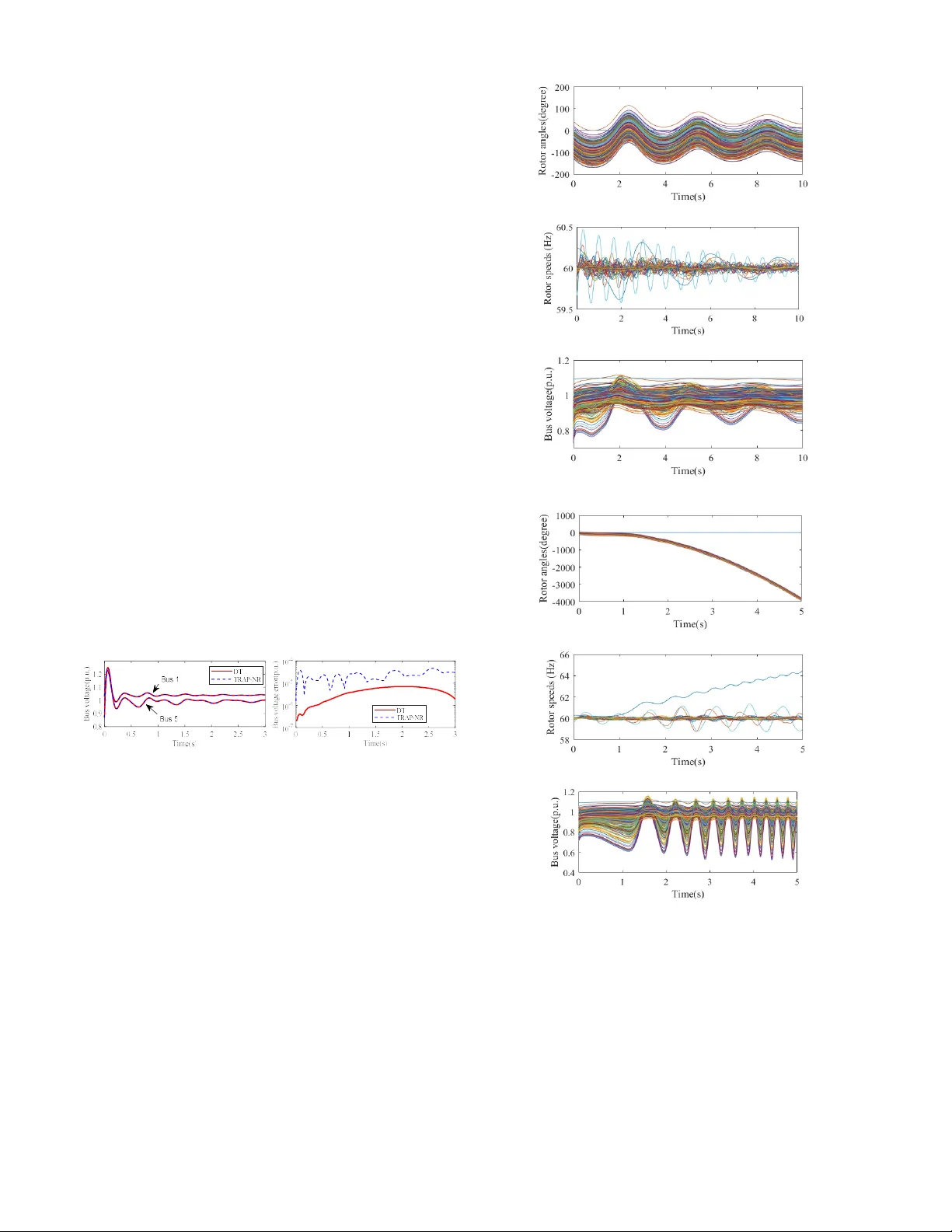
Accepted b y IEEE T ransactions on Power S ystem (DOI: 10.1 109/TPWRS.2 019.2945512) 1  Abstract — This paper proposes a novel non-iterative method to solve power system differential algebraic equations (DAEs) using the differe ntial transformatio n , which is a mathematical tool able to obtain p ower series coefficients by transformation rules instead of calculating high order derivatives and has prove d to be effective in solving state variables of nonlinear differe ntial equations in our previo u s st u dy. This paper f urther sol ves non-state vari ables, e.g. curren t injections and bus v olta ges, directly w ith a realistic DAE model of pow er g rids. These non-state variab les, nonlinearly coup led in network eq uations, are conventionally solved b y numerical methods wit h time-consuming iterations, but their differential tra nsformations are proved to satisfy formally linear equa tion s in this paper. T hus, a non-iterative algorithm is designed to analytically solve all variables of a power system DAE model with ZIP lo ads. From test results on a Polish 2383-bu s system, t he proposed method demonstrates fast and reliable ti m e p erformance compared to traditional numerical approaches including the implicit trapezoidal rule m ethod and a pa rtition ed scheme using the explicit m odified Euler method and New ton Raphson method. Index T er ms —Di ffere ntial algebraic equations; Differential transformation; numerical i ntegration; pow er syste m simulation; time domain simulation; transient sta b ility. I. I NTRODUCTION OVLING po w er s ystem di fferential algebraic e quations (DAEs) is a fu ndamental comp utation ta sk o f time do m ain simulatio n to assess the transie n t stabilit y of a p ower s ystem under co ntingencies. T raditionally, t he differe ntial equat ions are solved by a numerical integration method, and the alg ebr aic network equat ions are solve d by a numerical i teration metho d at each integration step [1]-[4 ]. These methods m ay suffer f ro m huge computation burd ens caused b y the iterations at each integration step for the co nvergence o f the network equations and t he large number of integratio n st eps to ens ure the accur acy and numerical stability of solvi ng the differential equat ions. Moreo ver, the computation speed can further deter iorate when system states c hange signific antly, or the syste m model has strong nonlinearity since the network equation is more diffic ult or even fail s to converge b y num erica l iteration met hods. Many researc hes are conducte d in the literature to a ccelerate the solv ing proc ess of p ower s y stem DAEs, falli ng into This work was supported in part by the ERC Progr am of the NSF and DOE under NSF Grant EEC-104 1877 and in part by NSF Grant ECCS-161002 5. Y. Liu and K. Sun are with the Department of EECS, University of Tennessee, Knoxville, TN 37996 USA (e-mail: yliu161@vols.utk.edu , kaisun@utk.edu ). following thre e categories: 1) model simplific ation, 2) parallel computing, and 3 ) sem i-anal y tic al methods. In the first categor y , both the differe ntial equations a nd algebr aic equations of a D AE model can be simplified. For instance , a widely used coher ency-based model reduction tec hnique aggregates a gro up o f c oherent genera tors into an equi valent generator [5 ]-[6]. Also, to avoid solving nonlinea r algebraic network equations separat ely from sol ving differenti al equations, many simulatio n tools assu me all constant impedance loads so as to e limi nate the networ k equations of a DAE model a nd obtain an ordinar y di ff erential e quation mode l [3],[7] . Ho w e ver, methods of this category can bring substantial error s in simula tion. T he second cate gory of methods employ p arallel co m puters to spe ed up s imulation, which d ecompose the DAE model or co mputation ta sks onto multiple processors such as the Pa rareal i n time met hod [8]-[9], multi-deco mposition approac h [10], the domain decomposition method [11]-[1 2], the waveform relaxation method [13], the instantaneou s relaxation me thod [14 ]-[15], the multi-area Thevenin equivale nt metho d [ 16]-[17], a nd the p ractical parallel impleme ntation techniques in [7 ], [18] -[19]. How e ver, these methods still rely o n the traditional numerical al gorithms to solve DAEs, t hus still requiring small -enough integrati on steps a nd numer ical iteratio ns. Methods of the third category shift so me of co mputation bur dens fro m the o nline sta ge to the offline stage, such as the semi -an al y t ical methods rece ntly proposed by [ 20]-[24] that o ffline de rive appr oximate, analytical solution s of dif ferential equa tions for the purp ose o f online simulation. Ho wev er, network equat ions with a D AE model still ne ed to be solved by iterative numeric al methods. In this paper, a novel non-ite rative m e thod is proposed to solve the D AE model of a la rge-scale p ower system u si ng a differential transfor mation (D T) method [ 25]-[26], which has proved to be an effective m athematical to ol to solve state variables of po wer syste m differential equati ons in our pre vious work [2 7]. First, this pape r der ives t he DT s of the algebraic network e quations with curre nt injectio ns. Then, we prove that current injections and bus voltages which are coup led b y t he original nonlinear net work eq uations, satisfy a for m a lly li near equation i n terms of t heir power series coefficients after DT. Further, a non-iterative algorithm is designed to analytically solve both state variables and non-state v a riables b y po wer series o f time. Simulatio n result s sho w the propo sed method is fast and reli able compared to traditional met hods. The rest of the pap er is organized as follo ws. Sect ion II conceptually descr ibes the pro posed method . Section II I Solving Power Syst em Dif ferential Algebra ic Equations Using Dif ferenti al T ransform a tion Yang Liu, Student Member, IEEE , Kai Sun, Senior Me mber, IEEE S Accepted b y IEEE T ransactions on Power S ystem (DOI: 10.1 109/TPWRS.2 019.2945512) 2 derives the D Ts of the po w er system DAE model. Sec tion I V designs a non-iterati ve algorithm using the derived DT s. Section V tests the p roposed method on a Polish 2 383-bus system. Final ly, conclusion is drawn in Sectio n VI. II. P ROPOSED M ETHOD FOR S OLVI NG P OWER S YSTEM DAE M ODEL U SING D IFFERENTIAL T R A NSFORMATION A. Intro duction of the Differential Transfo rmation The Differential Tra nsf o rmation (DT) method is an emerging mathematic al too l that is developed in app li ed mathematic s and is introduced to the power system field in [27]. For a linear or nonline ar function x ( t ), its DT X ( k ) is defined in (1), meanin g the k th order p ower series coefficie nt of x ( t ), where t is an indep endent variable su ch as time and k is the po w er series o rder . A major advantage of t he DT method is that it can directly obtain any order p ower se ries coefficie nts b y its various transfor m ation rules, witho ut complica ted high-orde r derivative oper ations.         0 0 1 ! k k t k k d x t X k k dt x t X k t                 (1) B. Con ceptual Descriptio n of the Propo sed Method A power syste m DAE model in the s tate-space representation is give n in ( 2), where x is the state vecto r, v is the vector of bus voltages, f repre sen ts a vector f ield dete rmined by d ifferential equatio ns on dynamic device s suc h as synchronous ge nerators a nd associated controller s, i is the vector-valued function on c urrent inj ections f r om a ll ge nerators and load buses, , and Y bus is the net w o rk admittance matrix.      bus x = f x, v Y v i x, v  (2) In the pro posed method, the solution o f both state variables and the non- state variables, b us voltages, are app roximated by K th or der power serie s in ti me in (3). The major task is to solve po w er series coe fficients of o rders f r om 0 to K . The two steps to obtain these c oefficients a re co nceptually shown belo w a nd then elaborat ed in Sections II I and IV, respe ctively.     0 0 K k K k k t k t     x X v V (3) 1) Step 1 : Deriving DTs o f Power System DAE Mod el The DT s of the DAE model (2 ) w ill be derived in Section III and have the general for m i n (4). Compar ed with the original DAE mode l (2) , ea ch variab le or function x , v , f , i a re transfor m e d to t heir p ower series coefficie nts X ( k ), V ( k ), F ( k ) , I ( k ) (denoted by their co rresponding capital l etters), coupled by a n e w se t of eq uations in ( 4). It can be obser ved that, the left-hand side (LHS) of (4) only contains th e ( k +1) th order coefficients of state var iables and k th ord er coe ffi cients o f b us voltages, respe ctively, while the right-hand side (RHS) couples 0 th to k th order coefficients of both state variables and bus voltages b y nonlinear function s F and I .       ( 1 ) 1 ( ) ( ) ( ) , 0 (a) ( ) ( ) ( ) ( ) , 0 (b) k k k l l l k k k l l l k         bus X F F X , V Y V I I X , V   (4) 2) Step 2 : Solving Power S eries Coefficients of State Variable s and Bus Volta ges The main task i n this step is to sol ve power ser ies coefficients X ( k ) and V ( k ) ( k  1) from the ( k -1) th o rder coefficients, as indic ated b y t w o cir cled numbers in Fig. 1 . Thus, any o rder coefficients ar e solvable from X (0) and V ( 0). Fig. 1. Recursive proce ss to solve power s eries coefficients Rewrite (4a) as ( 5) by rep lacing k by k -1. Note that X ( k ) only appear s on the LHS and the RHS onl y contains coefficients up to order k -1. There f ore X ( k ) can be explicitly solved from calculated lower order coefficients.     1 ( ) ( ) , 0 1 k l l l k k    X F X , V  (5) In contrast, from (4 b), so lving V ( k ) is not straight forward since it appears on bot h the LHS and RHS and t he vector-valued function I ( · ) is nonlinear. Lat er in Section IV, we will prove th at the coefficients of current injection I ( k ) satisfy a formally li near equation (6) about V ( k ).     1 2 1 1 2 2 ( ) ( ) ( ) ( ) 0 , ( ) ( ) 0 1 k k l l l k l l l k                      I A V B A A X , V B B X , V   (6) Note that the matrice s A a nd B still contai n nonlinear functions that o nly involve the ( k -1) th and lower order coefficients on b us volta ges, so the y do not affect the solvability of V ( k ). Finally, V ( k ) is ex plicitl y s o lved in (7) after substituting ( 6) into (4b ). T he detailed de rivation of matrices A and B is pre sented in Sectio n IV.   1 ( ) k    bus V Y A B (7) For complex variables and parameters in (2)-(7) such as current injection vector i , bus voltage vector v , DTs I ( k ) and V ( k ), and ad mittance matrix Y bus , their real and imagi nary parts are sepa rate as follows, wh e re N is t he number of b uses.                     , 1 , 1 , , , 1 ,1 , , , 1 , 1 , , , 1 ,1 , , 11 1 1 , , , , , , , , , where T x y x N y N T x y x N y N T x y x N y N T x y x N y N N ij ij ij ij ij N NN i i i i v v v v k I k I k I k I k k V k V k V k V k G B B G                                                   bus i v I V Y Y Y Y Y Y          Remark: T here ar e two i m po rtant observatio ns: 1) from (6) that curr ent injec tions and bus voltages, which are c oupled by nonlinear network equations in (2), t urn out t o hav e line ar relationships i n terms o f their coef ficients after DT; 2 ) Accepted b y IEEE T ransactions on Power S ystem (DOI: 10.1 109/TPWRS.2 019.2945512) 3 coefficients o n bus voltages ca n be explicitly solved by (7) and then u sed to cal culate bus voltages by ( 3) in a straightforw ard manner, whic h is di fferent from using a conventio nal power flow sol ver to calculate bus voltages by numerical iteratio ns. The proposed DT ba sed method for solving DAEs differentiate s i tself from t he tr aditional solution schemes which rely o n iterati ve numeric al met hods such as the famil y of Newton Rap hson (NR) metho ds. III. DT S OF P OWER S YSTEM DAE M ODEL Typically, a power s y ste m D A E model contai ns differentia l equations for each gene rator a nd its co ntrollers, curre nt injection e quations for all generato r and load buses, and the transmission net work equation. DT s of differential eq uations are provide d in [27] and DTs of current injectio n equations a nd the networ k equation are d erived in this section. A. Vecto rized Transformatio n Rules In po w er system D AE mode l, currents a nd voltages are usually writte n as matri x forms usi ng rec tangular c oordinates. To make the e xpression of the d erived DT more c ompact, this section e xtends t he existin g tra nsformation r ules for scalar valued functi ons to vectorized transformation rules so a s to be directl y app lied to a vector valued function without expa nding it into ma ny scalar val u ed functions first. The pr oposition 1 provide s six vec torized transfor mation rules in (8) for vector or matrix op erations that often appea r in a p ower system DAE model. These rules can be easily obtained by applying the existing transfor m ation rules to each elemen t of the vec tor valued functio n and their pr oofs are omitted . Propositio n 1: Given x ( t ) and y ( t ) as vector- valued functio ns having DT s as X ( k ) a nd Y ( k ), h ( t ) and H ( k ) as a scala r functio n and its DT, and c a nd d are constant matrices, the transfor m a tion rules in ( 8) hold.                         0 1 0 i ) ( ) ( ) ( ) ( ); ii ) ( ) iii) ( ) ) ( ) ; i ) ( ) ( ) 1 ) ) v v 1 vi 0 ( T m m T k k t t k k k k t m k m k H t k k t t t m t k k t m H h                                  x y X Y x cx cX x d X x y y X d X Y X Y Y Z (8 ) B. DTs of the Current Injec tion Equa tion of Generato rs Consider the d etailed 6 th order synchrono us generator model in [27 ]. T he c urrent inje ction u sin g the d - q coordinate system is given in ( 9). T he co ordination transformation between d - q and x - y co ordinate system i s give n in (1 0). Va riables i d , i q ar e the d -axis and q -axis stator curren ts; e’’ d , e’’ q are d -axis and q -a xis sub-transient volta ges; v d a nd v q a re the d -axis and q -axis terminal voltages; δ is the rotor angle. Parameters x’’ d , x’’ q and r a are the d -axis and q -axis sub-transient reactance a nd internal resistance, r espectively. 1 '' '' '' '' , where d d d a q q q q d a i e v r x i v e x r                                                            a a y y (9) , , where x d x d y q y q i i v v sin cos i i v v cos sin                                                           r r r (10) The current injectio n under the x - y a x is is give n in ( 11) by combining (9 )-(10). '' '' , where x d x y y q i e v i v e                                          a T ry r      (11 ) The DT of (11) is given i n (12).                 '' '' x d x y y q I k E k V k k k I k V k E k                                     ( 12) For deta ils of the de rivation, the RHS o f (12) is ob tained using rule s i) and v), where t he Γ ( k ) and Λ ( k ) are respectivel y DTs of τ and λ , given by rule s ii) , iv) and v) as follows. R ( k ) is the DT o f the matrix r , where Φ ( k ) and Ψ ( k ) are DT s of sine and cosine function s, respectivel y , give n in Pro position 2 in [27].     k k    a a ry R y         T k k k     T r R     ( ) ( ) ( ) ( ) ( ) k k k k k                R Eq. (12) co ntains the convolution of a 2×2 matrix and a 2×1 vector, and its calculation is the sam e as the convolution of two matrices i n the rule v). T he detailed expr ession is following.                 '' '' 0 0 k k x d x y y m m q I k E k m V k m m m I k V k m E k m                                           C. DTs of the Current Injectio n Equa tion of Loads Consider the ZIP lo ad model [ 3] in (13) where p and q are the active and reactive power loads, respectivel y; v t is the bus voltage magnitude defined in (14 ) and u e q uals its s quare; p 0 , q 0 and v t0 are t he stead y state acti ve po w e r, r eactive po w er and b us voltage; a p a nd a q ar e the pe rcentages of consta nt i m peda nce load; b p and b q are the percentages o f co nstant current load; and c p and c q ar e the pe rcentages of co nstant po w e r load . There are a p + b p + c p =1 and a q + b q + c q =1. 2 0 0 0 2 0 0 0 ( ( ) ( ) ) ( ( ) ( ) ) t t t t t t q t p p p q q t v v p p a b c v v v v q q a b c v v                      (13) 2 2 , t x y v v u u v    (14) The current inje cted to the net w ork can be calculate d fro m the acti ve and rea ctive power i njections, and i s writte n in mat rix forms in (15) where β a , β b and β c are co nstan t matric es. 2 0 0 1 1 1 1 x x x x y y y y x x x a b c y y y t t t i i i i i i i i v v v v v v v v u v                                                                            z i p     (15) 0 0 0 0 0 0 0 0 0 0 0 0 , , p q p q p q q p q p a b c q p p a q a p b q b p c q c q a p a q b p b q c p c                                        Accepted b y IEEE T ransactions on Power S ystem (DOI: 10.1 109/TPWRS.2 019.2945512) 4 DTs of u and v t are derived in [27] and are given in (16)-(17 ) . T hen, DT s of the RHS te rms in (1 5) ca n b e obta ined using rules in (8 ) as explained in t he following.           x x y y U k V V k k k k V V     ( 16)             1 1 1 1 V 2 0 2 0 k t t t t t m k U k V m V k m V V       (17) The first term i n RH S of (1 5) is the curren t i njection o f constant impedance load. It i s th e pro duct of a constant number 1/ v t0 2 , a constant matrix β a and a vector valued function [ v x , v y ] T . Ther efore, its DT is given i n (18) using the rule ii i).         2 2 0 0 1 1 x x x x a a y y y y t t i v I k V k i v I k V k v v                                            z z   (18) The seco nd ter m in RHS of (15 ) is the c urrent inj ection o f constant current loa d w it h DT in (19). I t is t r ansfor m e d b y thr ee steps. First, the product of the constant matrix β b and the v e ctor valued function [ v x , v y ] T is transfor m e d using the rule iii) . Then , the di vision of the vector va lued functio n β b [ v x , v y ] T and the scalar valued function v t is transfor med using the rule vi). Finally, the p roduct of the co nstant number 1/ v t0 and the vec tor valued functio n 1/ v t β b [ v x , v y ] T is transfor m ed usi ng the rule iii) .                 0 1 0 0 1 1 1 1 0 x x b y y t t k x x x b t y y y t t m i i v i v v v k V k i m V k m k V k v V I I i m                                                                          i i   (19) The third term i n RHS o f (15 ) is the c urrent inj ection o f constant p ower load. It conta ins the pr oduct of a constant matrix β c and a vecto r valued function [ v x , v y ] T , then divided b y a scala r valued fu nction u . Si milar with the consta nt c u rrent load, its DT is given in (20) using rules iii) and vi).                 1 0 1 1 0 x x c y y k x x x c y y y m i I v i v u k V k m U k m k V k m U I I I                                                                          p p p   (20) Finally, t he DT of c urrent injection equation (1 5) is given in (21) b y s umming DT s of each term (18 )-(20) using the rule i) .                 x x x x y y y y I k I k I k I k I k I k I k I k                                            z i p ( 21) D. DTs of th e Network Eq uation The network e quation is in (22 ), which couples the current injections of all generators a nd loads. It s D T is give n in (23).     , , RHS of 11 for generator buses RHS of 15 for load bus es RHS of (11) RHS of (15), for bus es w ith bo th generators and loads x m y m i i                              bus bus i Y v (22)                 , , RHS of 12 fo r genera tor buses RHS of 21 for load bu ses RHS of 12 RHS of 21 for buses with both generators and loads x m y m k k I k I k                              bus I Y V (23) IV. S OLVING P OWER S ER I ES C OE FFI C IENTS OF S TAT E V ARIABLES AN D B US V OLTAGES A. Linea r Relationship Between Current In jection an d Bus Voltage in terms of Po wer Series Coefficient s Propositio n 2 : T he transformed current injections i n (12) and (21) for generator s and loads respectively satis fy equations (24) a nd (25), which are for mally linear.         x x y y I k V k I k V k                       g g A B (24 )         x x y y I k V k I k V k                       l l A B ( 25) The pro ofs are given in Appendix a nd the detailed expressions of matrices A g , B g , A l a nd B l a re in (36) and (40). Using thi s pr oposition, curr ent i njections of al l buses can be written as (6 ) with A and B i n (26).   1 2 1 2 , fo r g e n e ra t o r b u s e s , fo r l o a d b u s e s , , , fo r b u s e s w it h b ot h g e n e ra t o r s a n d lo a d s , fo r g e n e ra t o r b u s es , fo r l o a d b u s e s , , , fo g l N n g l g T l T T T N n g l d i a g                              A A A A A A A A A B B B B B B B B B   r b u s e s w i t h b o t h g e n e ra t o r s a n d lo a d s                (26) B. Non -iterative Algorithm to Solv e Power Series Coefficients Following the basic idea in Fig. 1, Alg orithm 1 is further designed to solve po w er serie s coeffic ien ts of both state variables and bus voltages up to any desired order. Note th a t all the coefficie nts are explic itly calculated with no iteration. Algorithm 1: Solve Coefficients Input : initial values of state var iables and bus voltages 0 0 , x v Output : any or d er coefficients     , , 0 k K k k  X V  Steps : Initialization:     0 0 , 0 0   X x V v 1. Calculate the matrix A 1.1 Calculate the matrix g A for generators by (36) 1.2 Calculate the matrix l A for loads by (40) 2. Calculate the matrix    bus Y A and solve   1   bus Y A for 1 : k K  3. Solve   k X :     1 ( ) ( ) , 0 1 k l l l k k    X F X ,V  using [27] 3.1 Solve state variable s of governors and turbine s by (8) a nd (10) in [ 27] 3.2 Solve state vari ables of 6 th order g enerator model by (17) in [27] 3.3 Solve state vari ables of IEEE Ty p e I exciter model by (24) in [27] 4. Calculate the matrix B Accepted b y IEEE T ransactions on Power S ystem (DOI: 10.1 109/TPWRS.2 019.2945512) 5 4.1 Calculate the matrix g B for generators by (36) 4.2 Calculate the matrix l B for loads by (40) 5. Solve   k V :   1 ( ) k    bus V Y A B end C. Exten sion This section furt her d iscusses the linear re lationship among non-state variables for a frequency dep endent load model. When co nsidering the i mpact of fre quency changes, the Z IP load model is c hanged to a set of DAEs in ( 27), where θ is the bus voltage angle, Δ f is the frequency c hange, i l is the c urrent injection of the ZIP load m odel, i l,f is the current inj ection after considerin g the frequency cha nge, and d is a constant. , ( 1 ) l f l f d f       i i  ( 27) The DT o f (27) are given in (28)-(29 ). For the DT o f the algebraic current inj ection eq uation ( 29), it is also pr oved to satisfy a formally linear e quation in (30) w ith d etailed proo fs given in the App endix. 1 ( ) ( 1 ) k F k k     (2 8) , ( ) ( ) ( ) ( ) l f l l k k d k F k     I I I (29) , ( ) ( ) ( ) l l f l f k k F k                      l V I A A B (30) Two ad ditional variables are introd uced, i.e., the state variable θ and the non-state variable Δ f , and their sol utions are also appro ximated b y po wer series of time i n (31), where the coefficients Θ ( k ) a re solved to g ether wit h the co efficients of state variab les X ( k ) and coe fficients Δ F ( k ) are solved to gether with the co efficients of bus voltages V ( k ) .     0 0 ; K K k k k t f F k t         ( 31) V. C ASE S TUDY The p roposed method i s first illustra ted on a 3-machine 9-bus po w er system. T hen, to vali date the a ccuracy, t ime performance a nd r obustness of the propo sed method on solving practic al high-di mensional no nlinear DAEs, the 327-mac hine 2383 -bus Polish syste m [29] w ith deta iled model s o n generators, excite rs, governors, turbines, a nd ZIP loads are used. In t he ZIP load model, the percentages o f each co mponent are 20% , 30% and 50% r espectively. Two widely used solution ap proaches a re implemented for compariso n [3 ]: 1) TRAP-NR method where the dif ferential equations are algebraized by i mplicit trape zoidal metho d (T RA P ) first and then sol ved simulta neously with the ne twork equations b y Ne wton Rap hson (NR) method. 2) ME-NR method using a partitio ned sc heme where the differenti al and network equations are alternatively solved by explicit modified Euler m etho d (ME) an d N R method r espectively. The ti m e step length o f both the T RAP-NR method and ME -NR method is 1×10 -3 s, while the p roposed method pr olongs the ti me step length to 10 times and still a chieves better a ccuracy. For a fair comparison, the b enchmark result is g iven b y the TRAP-NR method using a small e nough time step le ngth of 1×10 -4 s a nd e rrors of the pro posed method, the TRAP- NR method and the ME-NR method are calculated by their differences from t he benc hmark res ult. Simulatio ns ar e conducted in M ATLAB R201 8b on a personal computer with i7-6700 U CPU. A. Illustrat ion on a 3-machine 9-bu s Power System The 3-machine 9-bu s po w er syste m in [ 28] is used to illustrate the p roposed method . The system contai ns generators at b uses 1 t o 3 equippe d with gover nors and exciter s whose differential equatio ns can be fo und in [2 7], ZIP loads a t buses 5, 6 and 8 and transition b uses 4, 7 and 9. Equatio n (32 ) sho ws the network eq uations on curre nt injections: '' , , '' , , 2 2 , , , , , , 0 2 2 , 2 , , , 0 , , , , , , 1 , 2 , 3 1 1 1 , 1 t d n x n n n y n c x n y n x n x n x n a n b n y n y n n q n x n y n y n t n x n y n i if n i i v v i v v v v v v v v v v e e                                                                          , , , , 11 19 91 99 ,1 , 1 9 ,9 , 5 , 6 , 8 x x y x y n n y n v if i n v i v v                                                       Y Y Y Y        (3 2) Apply D T to (27) acco r ding t o ( 12), (18)-(21) . Coefficie nts of state variables a nd b us voltages, i.e. X (1), V ( 1),…, X ( K ), V ( K ), a re recursivel y calculated starting fro m X (0) and V (0). For illustration purpo se, calculatio n o f X (1) and V (1) is explained as follows. First, c alculate X (1) by (5) w it h k =1:     1 ( 0 ) (0 )  X F X , V where detailed equations of F can b e found in [27]. T hen, write I (1) of all ge nerators a nd lo ads as a linear equatio n abo ut V (1) so as to e xplicitly sol ve V (1). Fo r instance, c urrent injectio ns from t h e c onstant po w e r load component at bus 5 ( i.e. the last term o f the seco nd equatio n in (32) ) can be calculated by the following detailed steps. T he remaining curre nt i njections c an be handled in the similar wa y.                                 , 5 ,5 , 5 ,5 5 ,5 ,5 ,5 , 5 ,5 , 5 ,5 5 ,5 , 5 ,5 5 1 1 1 1 ( ) 1 1 1 1 2 1 0 0 0 (0) 0 0 (0) 1 0 1 x x x c y y y x x c x x y y y y I V I U a I V I V I V V V V V U U I                                                                                 p p p                                           ,5 , 5 , 5 , 5 , 5 ,5 ,5 , 5 ,5 ,5 , 5 ,5 , 5 , 5 , 5 ,5 ,5 , 5 5 ,5 , 5 5 0 0 0 0 (0) 0 0 0 0 (0) ( ) 1 2 0 2 0 1 1 ( ) 1 2 0 2 0 1 2 0 2 0 1 2 0 2 0 x x x x x c y x y y y x x x c x y y y y y y b V V I V I V c V V I V I V V I V I V I V U U I                                                                                ,5 ,5 , 5 ,5 ,5 , 5 ,5 ,5 1 0 ( ) 1 0 0. 87 71 0 .1 566 1 0 1 ( ) 0. 15 66 0 .8 77 1 1 0 1 x y x x y y V d V V V e V V                                                                              p p A B  (33) For load bus 5, the first order coefficie nt [ I x ,5 (1), I y ,5 (1)] p T for constant po w e r load is given in ( 33a) from (20) . After substituting the expre ssion of U ( 1) given i n (16) and simple matrix operatio ns , it turn s to (33b) and (33c), respectively. Then, all ter ms containing [ V x ,5 (1), V y ,5 (1)] T are combined as a group v e rsus th e re maining a s another group in (33d). Since β c,5 is a constant matri x a nd all variables, U 5 (0), V x ,5 (0), V y ,5 (0), I x ,5 (0), I y ,5 (0), except for [ V x ,5 (1), V y ,5 (1)] T have been known, their values are directl y substituted into the equation to have Accepted b y IEEE T ransactions on Power S ystem (DOI: 10.1 109/TPWRS.2 019.2945512) 6 (33e) . Again, [ I x ,5 (1), I y ,5 (1)] p T is formall y linear about [ V x ,5 (1), V y ,5 (1)] T with coefficie nt matrices d enoted by A p ,5 and B p ,5 . After obtaining the linea r f or ms for all current injections, we can co mbine them into the matrix representation ( 34). For instance, A 1 and B 1 are equal to the A g ,1 and B g ,1 respectivel y at generator bus 1.         , 1 ,1 ,1 9 1 9 9 ,9 1 1 1 1 x x y y I V I V                                                           B A B A     (3 4) Finally, combining (34) w it h the DTs o f the network equation ( 23), V ( 1) is explicitl y solved in (35 ). By recursivel y conducting t his pr ocess, coeffi cients of bus voltages and state variables with any order k can be o btained.     1 11 19 1 1 91 99 9 ,1 9 ,9 1 1 x y V V                                                                                 Y Y A Y Y A B B         (3 5) In ea ch time step, solutions o f involved varia bles are approximated by p ower s eries of tim e in ( 3). By perfor m in g the above proc ess in multiple ti me steps, the solution s over a desired simu lation r ange is obtained. Fig. 2a gives the trans ient voltage trajecto ries a t bus 1 and bus 5 after a large disturba n ce using both t he propo sed method w it h K =8 a nd time step le ngth of 0.0 1 s, and the T RAP-NR met hod with time step lengt h of 0.001 s. Fig. 2b f urt her pr ovides the maximum voltage er rors o f all 9 buses for b oth methods compared with t he bench mark result. I t shows that the err or o f the proposed m e thod i s r educed by one order of ma gnitude co mpared to that of the T RAP-NR method o ver the e ntire s imulation p eriod de spite the 10 ti mes prolonged time step length. (a) (b) Fig. 2. T rajectories and erro rs of bus voltages fo r th e 9-bus sy st em (a) Vol tage trajectories at bus 1 and b us 5 (b) Maximum voltage e rror of all 9 buses B. Accu racy and Time P erformance Both stable and unstable sc enarios are simulated for the Polish system to validate the accuracy and time perfor m ance of the propo sed method. Respectivel y for two scenarios, Fig. 3 and Fig. 4 respe ctively show the transient r esponses o f roto r angles, ro tor speeds a nd bus v olta ges simulated by t he proposed method. The machine 1 is selected a s the refer ence to calculate r elative roto r angles. The maximum error s o f rotor angles, ro tor speed s, and bus voltages co m pared with the benchmark results are 3. 02×10 -5 degree, 4.27×1 0 -7 Hz , 3.33×10 -7 p.u. for stable scenario and 2.02×10 -5 d egree, 3. 00×10 -7 Hz, 2.78×10 -7 p.u. for unstable scenario respectively. It shows the proposed m ethod can accuratel y si mulate bo th stab le and unstable contin gencies in the transient sta bility simulati on. (a) Rotor angles (b) Rotor speeds (c) Bus voltages Fig. 3. Trajectories of the stabl e scenario for the 2383-bus sy ste m (a) Rotor angles (b) Rotor speeds (c) Bus voltages Fig. 4. Trajectories of the unstable scenario for the 2383-bus system Tab le I gives the maximu m err ors of all state variable s (includin g rotor angles, rotor speeds, tr ansient and s ub-transient voltages, f ield voltages, etc.) and b us voltages r espectively, as well as the computation time per 1-second simulation. The errors of the state v a riables and the bus volta ges using the proposed m e thod are respec tively two orders of magnitud e lower and one order of magnitude lower than those usin g the TRAP-NR method and the ME-NR method . Also, the computatio n sp eed of the prop osed method is arou nd 10 times faster than t he other t wo methods. T hese results show t he proposed m ethod is more efficient a n d ac curate. Accepted b y IEEE T ransactions on Power S ystem (DOI: 10.1 109/TPWRS.2 019.2945512) 7 TABLE I C OMPARISON OF A CCUR A CY AND T IME P ERFORMANCE Scenarios Methods Error of state variables (p.u.) Error of bus voltages (p.u.) Computation time (s) Stable DT 2.69×10 -6 3 .33×10 -7 18.76 TRAP-NR 1.30×10 -4 1 .10×10 -6 176.43 ME-NR 2.63×10 -4 2 .26×10 -6 191.40 Unstable DT 1.89×10 -6 2 .78×10 -7 18.85 TRAP-NR 1.41×10 -4 1 .61×10 -6 182.76 ME - NR 2.79 ×10 -4 2.93 ×10 -6 196.02 Fig. 5 gi ves the error propagation alo ng the simulatio n proce ss for four scenarios with th e time ste p le ngth increa sed to 0.02 s, 0.05 s, 0.10 s and 0 .20s r espectively starti ng fro m the same initial state s at t =0. I t s hows that the err or does not accumulate much when the t ime step length is 0.02 s and 0.05 s. The maximum errors are in th e o rder o f magnitude of 10 -5 p.u. and 10 -3 p .u.. respectivel y. Fo r la rger ti m e step le ngths, the error becomes unne glectable when th e time step le ngth is 0.10 s and even r eaches 10 5 p.u. when the time step length i s 0 .20 s, indicting di vergence of t he solution. Fig. 5. Error propagation under different time step lengths In this pap er, the K is deter mined by grad ually increasing i ts value until the maximum err or of all variables satisfie s a pre-defined requir ement. T able II gives t he erro r and the computatio n time with differe nt val ues of K . It shows t hat t he errors of state variab les and bus voltages are decrea sed when K increases f r om 2 to 8. And, keeping incr easing K d oes not further improve the acc uracy much b ut brings mor e computatio n burden. Ther efore, K =8 is sele cted throughout t he case st u dy to meet the ac curacy r equirement, where the maximu m er ror of all variables is in the order of magnitude of 10 -6 p.u.. TABLE II A CCURACY AND T IME P ERFORMANCE FOR D IF FERENT V ALU ES OF K K Error of state variables (p.u.) Error of bus voltages (p.u.) Computation time (s) 2 2.70×10 -2 4.91×10 -4 8.78 3 8.51×10 -4 2.10×10 -5 10.31 4 3.33×10 -5 1.82×10 -6 11.82 8 2.69×10 -6 3.33×10 -7 18.76 12 2.69×10 -6 3.33×10 -7 27.91 Since a large computation burden w ith transient stability simulatio n lie s i n solvin g li near eq uations, both spa rse matrix and LU factorization techniq ues a re implemented in this paper for the DT method, TRAP-NR method a nd ME-NR met hod. Tab le I II compares t he total number N LU of times o f LU factorization with three methods in a 1 -second simulation. It is calculated by N LU = n LU × M , wh ere n LU is the n umber of ti mes of LU factor ization within ea ch ti m e step a nd M is the tota l number o f ti me steps. W ithin each time step , both the TRAP-NR and t he ME-N R met hod need to pe rform LU factorization for each ite ration unless a so -called ver y d ishonest NR method is a pplied, but the DT method o nly need s to perform L U factorization once . Also, the DT method only takes 1/10 o f time steps of the other two m ethods. Therefore, the DT method can significa ntly red uce t he number o f ti mes of LU factorization i n a simulatio n . TABLE III C OMPARISON OF N UMBER OF LU F ACTORIZATION Methods n LU M N LU = n LU × M DT 1 100 1 00 TRAP-NR 3.004 1 000 3004 ME-NR 2.060 1000 2006 C. Robu stness The rob ustness o f the p roposed method is validated in t hree sets of case s: 1) sta ble and un stable scenarios, 2) distur bances with differe nt severities, an d 3) different per centages of constant po wer load. By co mparing the results of s table and unstable scenarios in Tab le I, it is obser ved that the TRAP-NR met hod and ME-NR method are less accurate and slower in simulating the unstab le scenario than in the stable scenario, but the proposed D T -based method performs al most t he same in bo th sc enarios. T his is because the syste m sta tes change s ignifica ntly i n the unstab le scenario a nd the NR met hod takes more iteration s to conver ge. At e ach time step, the TRAP-NR method takes averagel y 3.004 iterations in the stab le scenari o and 3.118 iterations in the unstable scenario. For ME -NR met hod, it ta kes 2.0 60 and 2.132 iterations, respe ctively. I n co ntrast, the pr oposed method do es not require iterations in the solvi ng pr ocess, t hus ha ving b etter robustness on unstable scenarios. Fig. 6 g ives the time performance and the a verage number of iterations of the N R method under d ifferent dist urbances with increasing seve rities using the thre e methods. It shows the computatio n ti m e o f the pro posed method is al most the sa me for d iff e rent disturb ances, but b oth the TRAP-NR method and ME-NR method take lon ger time when simulati ng lar ger disturbance s due to the incre ased number of iterat ions. Fig. 6. Robustness agai nst different disturbances Accepted b y IEEE T ransactions on Power S ystem (DOI: 10.1 109/TPWRS.2 019.2945512) 8 The time per formance a nd the average number of iter ations of t he NR method under di fferent per centages of constant po w er load is in Fig. 7. The h igher perce ntage of co nstant po w er load b rings stronger nonlinearity to the DAEs, thus making the N R method more difficult or fail to conver ge. In Fig. 7, t he c omputatio n ti me o f b oth the TRAP-NR method and ME-NR method increase significantl y with the hig her perce ntag e of the consta nt power load . B ut the pro posed method doe s n o t need iterations and its computation ti me is not affected much, showin g it is more rob ust to handle the str ong nonlinearit y caused by consta nt power load. Fig. 7. Robustness agai nst different perce ntages of constant power lo a d VI. C ONCLUSION In this paper, a DT based non-iterati ve method is prop osed for solving po w er syste m DAE s. Curr ent i njections a nd bus voltages coupled by nonli near network equatio ns in the origi nal state sp ace re presentatio n are proved to sa tisfy a formall y linea r equation i n terms of t heir power series coefficients after DT. Benefitin g from this propo sition, solutio ns of bot h state variables and non-state volta ges are calculated by po w er series of time whose c oefficients are explicitly solved using the designed algorithm with no iteration. Simulation results shows the pro posed method e ffectively r educes the computation burden co m pa red to traditional numerica l met hods and demonstrate s reliable time perfor mance whe n solving DA Es under large dist urbances or with strong nonlinear ities. A PPENDIX Proof o f (24) in P roposition 2 : Rewrite equatio n ( 12) as follows. Define A g and B g as (3 6). It is easy to co nfirm that A g and B g do not d epend on V x ( k ) and V y ( k ) .                       1 '' '' 0 0 k x d x x y y y q m I V m k k k E k V k m I k V V E k m k                                                                  1 '' '' 0 , 0 k d x y q m E k V k m V m E k k m                              g g A B    ( 36) Proof of (25) in Proposition 2: To prove (2 5), we onl y need to pro ve e ach co mponent o f the ZIP loa d in (18) - (20) c an be written into following three e quations, respectivel y.         x x y y I k V k I k V k                       z z z A B ,         x x y y I k V k I k V k                       i i i A B         x x y y I k V k I k V k                       p p p A B Part a) The DT of current i njections of constant impedance load (18) can be e asily writte n into ab ove for ms, by defining A z , B z as (37) . 2 2 2 0 1 , a t v    z z A B 0  ( 37) Part b ) The DT of current inj ections o f co nstant c urrent load ( 19) is rewritten as follo ws.                                   2 2 2 1 0 0 1 0 0 0 1 ,1 ,1 2 1 1 1 1 1 0 0 k x x x b t y y y t m i k x x x b t t y y y t t t m i i x y I k V k I m V k m I k V k I m v V k I m I V k m V k V k I m I v v v V k V k                                                                                                      i i i A B          2 0 0 0 x t y t i I V k I v           The third ter m can be furt her written as follo ws a fter substituting V t ( k ) in (17 ).                       1 3 0 0 1 ,2 3 2 0 1 0 0 0 0 0 0 1 2 1 2 k x x t t t y y t t m x y t I I V k U k V m V k m I I v v I U k I v                                                         i i i i B  The f ir st te rm can b e further written as follo ws afte r substituting U ( k ) in (16) .                                                   3 3 0 0 1 1 3 0 1 1 3 0 ,3 , 2 1 1 2 2 1 0 0 0 0 0 0 0 0 0 2 1 0 x x y y x t t k k x y t m m x y x x y y x y t x x y x y y y I I U k V V k V V k I I v v I V m V k m V m V k m I v I V k k k V V V k I v V k V k                                                                                   i i i i i i B A          ,2 3 0 1 0 , where 0 , 0 0 y x x y t I V V I v                         i i A Finally, define A i and B i as (3 8). It is ea sy to confirm that A i and B i do not d epend on V x ( k ) and V y ( k ) . ,1 ,2 ,1 ,2 , 3 + ,     i i i i i i i A A A B B B B (3 8) Part c ) Equation (20) is written as follo ws.                                   1 2 2 0 2 2 1 0 0 0 0 0 1 ,1 ,1 1 1 1 1 0 1 0 k x x x c y y y t m k x x x c y y y t t t m x y t I k V k I U k m I k V k I v V k I I U k m U k V k I I v v v V k V k m m m m v                                                                                                      p p p p p p A B          2 0 0 x y I U k I           p The third ter m can be furt her written as follo ws a fter substituting U ( k ) in (16). It is easy to c onf irm that A p and B p defined in ( 39) do not dep end on V x ( k ) and V y ( k ) .                                         0 1 1 0 1 1 0 ,2 ,2 , 2 2 0 2 2 2 1 1 , whe 0 0 0 0 0 2 0 r 0 0 0 2 e 0 x y t k k x y t y m m x y t x x x y x x y t x x y y y I U k I v I V m V k m V m V k m I v I V V k V V k I v V k I V V k I v                                                                                      p p p p p p p B A A      0 , 0 y V       ,1 ,2 ,1 ,2 + ,    p p p p p p A A A B B B (39) Finally, (25 ) is proved b y defining A l and B l as (4 0). Accepted b y IEEE T ransactions on Power S ystem (DOI: 10.1 109/TPWRS.2 019.2945512) 9 l z i p l z i p A A A A B B B = + = + + B + ( 40) Proof of (30): Rewrite (29) as follows. , 1 1 ( ) ( ) ( ) ( ) ( 1 (0 ) ) ( ) (0 ) ( ) ( ) ( ) ) l f l l k l l l m k k d k F k d F k d F k d m F k m                I I I I I I Since ( ) ( ) l l l k k   l I A V B has been proved for the ZIP load model, the a bove equatio n is further re w r itten as follo ws. , 1 1 1 1 ( ) ( 1 (0 ) ) ( ( ) ) ( 0 ) ( ) ( ) ( ) ) ( 1 ( 0 ) ) ( ) ( 0 ) ( ) ( 1 (0 ) ) ( ) ( ) ) l f l l l k l m k l l l l m k d F k d F k d m F k m d F k d F k d F d m F k m                           l l I A V B I I A V I B I Finally, by de f ini ng , , l f   l A A B in (4 1), the linear relationship (30) is satisfied, where , , l f   l A A B do not dep end on V x ( k ) and V y ( k ). 1 1 ( 1 (0)) ; (0 ); ( 1 (0 )) ( ) ( ) ) l l f l k l m d F d d F d m F k m                l l A A A I B B I (41) R EFERENCES [1] P. Kundur, N. J. Balu, M. G. Lauby, Power system stability and control . McGraw-hill New Y ork, 1994. [2] B. Stott, “Power system dynamic response calculations,” Proc. of th e IEEE , vol. 67, no. 2, pp. 219–241, 1979. [3] F. Milano, Power system modelling and scripting . Springer Sc ience & Business Media, 2010. [4] F. Milano, “On current and powe r injection models for angle and voltage stability an aly si s of p ow er s y stems,” IEEE Trans. Power Syst. , vol. 31, no. 3, pp. 2503–2504, May 2 016. [5] J. H. Ch ow , Power system coherency and model reduction . Springe r, 2013. [6] D. Osip ov, K. Sun, " Adaptive nonlinear model reduction for fast p ow e r system simulation, " IEE E Transacti ons on Power Systems , vo. 33, n o. 6, pp. 6746-6754, Nov . 2018. [7] S. Jin, et al, "C om p arative imple mentation o f high performance computing for power s ystem dynamic simulations," IEEE Trans. S mar t Grid, vol. 8, no. 3, pp. 13 87-1395, 2017. [8] G. Gurrala, et al, " Parareal in time for fast power system d ynamic simulations," IEEE Trans. P ower Syst ., vol. 31, n o. 3, pp. 1820-1830, J ul. 2015. [9] N. Duan, et al, "Applying reduced generator models in the coarse solver of parareal in time paralle l power system simulation," i n Proc. IEEE PES Innovative Smart Grid T echnologies Conference Europe , 2016, pp. 1- 5. [10] S. Zadkhast, J. Jats kevich, E. V aahedi, "A multi-decomposition a pproach for a cceler a ted t ime-doma in simulation of transient stability p roblem s," IEEE Trans. on Pow er Syst ., vol. 30, no. 5, pp. 2301-2311, Sep. 2015. [11] P. Aristidou, et al, "Power s ystem dynamic simulations u sing a p arallel two-level Schur-compleme nt decomposition," IEEE Trans. Power Syst ., vol. 31, no. 5, pp. 3984-3 9 95, Sep. 20 1 6. [12] P. Aristidou, et al, "Dynamic Simulation of Larg e-Scale Power S ystems Using a Parallel Schu r-Com p leme n t-Based Decomposition Method," IEEE Trans. P arallel & Distrib uted Syst., vol. 25, no. 10, pp. 2561-2570, 2014. [13] Y. Liu, Q. Jiang, "Two-stage parallel waveform relaxation method for large-s cale power system transient stabili ty simulat ion," IEE E Trans. Power Syst. , vol. 31, no. 1, p p. 153-162, Jan. 2016. [14] V. Jalili-Marandi, V. Di na vah i, "I n stantaneous relaxation-based real-time transient stability simulation," IEEE Trans. Power Syst., vol. 2 4, n o. 3, pp. 1327-1336, 2009. [15] V. Jalili-Marandi, e t al, "L arge-Scale Transient Stabili ty Simulation of Electrical Powe r Systems on Parallel GPUs," IEEE Trans. Parallel and Distributed Systems, vol. 23, no. 7 , pp. 1255-1266, 2012. [16] M . A. Tomim, et al, "Parallel tran s ient s tability si mulation b ased on multi-area Thévenin equivalents," IEEE Trans. Smart Grid, vol. 8, no. 3, pp. 1366-1377, 2017. [17] M . A. Tom im, J. R. Martí, T. De Rybel, L. Wang, and M . Yao, "MAT E network tearing techniques for multip roce ssor solution of large power system n etwor k s," in Power and E ne rg y Soc iety Gener a l M eeting, 2010 IEEE , 2010, pp. 1-6: I E EE. [18] R. Diao, S. Jin, F. Howell, "On p aral lelizing single d y namic simulation using HPC techniques and APIs of comme rcia l software," IEEE Trans . on Power Syst ., vol. 32, no. 3, pp. 2225-2233, May . 2017. [19] I. Ko nstantelos, et al, "I mp lementation of a massively parallel dynamic security assessment platfo rm for larg e-scale grids, " IEEE Tra ns. on Smart Grid , vol. 8, no. 3, pp. 14 17-1426, May 2 017. [20] N. Duan, K. Sun, "Power s y st em simulation using the multi-stage Adomian Decomposition Method," IEEE Trans. on Power Syst ., vol. 32, no. 1, pp 430-441, Ja n. 2017. [21] G. Gurrala, D. L. Dinesha, A. Dimit r ovski, et al, "Large multi-machine power s y stem simulations using multi-Stage Adomian Decomposition," IEEE Trans. Power Syst ., vol . 32, no. 5, pp. 3594-3606, Sept. 2017. [22] B. W ang, N. Duan, K . Sun, “A T ime-Power Series B ased Semi-A nalytical Approach for Power System Simulation,” IEEE Trans. Power Syst. , vol. 34, No. 2, pp. 841-851, March 2019 [23] C. Liu, B. Wang, K. Sun, "Fast power system simulation using semi analytical solutions ba se d on Pade Approximants," in Proc. Power and Energy Society General Meeting , 201 7 , pp. 1-5. [24] C. Liu, B. Wang, K . Sun, “Fast Po wer System Dynamic Simulation Us ing Continued Fractions,” IEEE Access , vol. 6, No. 1, pp. 62687-62 698, 20 1 8 [25] E. Pukhov, G. Geor gii, "Differential transforms and circuit theory," International Journal of C ircu it Theory and Applications , vo l. 10, no. 3, pp. 265-276, Jun. 1982. [26] I. H. A. Ha ssan, "Application to differential transformation method for solving systems of di ffer ent ial equations," Applied Mathematical Modelling , vol. 32, no. 12, pp. 2552-2559, Oct. 2007. [27] Y. Liu, K . Sun, R. Yao, B . Wa ng, "Po wer system time domain simulation using a differential transformation method," IEEE Trans. Power Syst. , vol. 34, no. 5, pp. 3739-3 7 48, Sept. 2019. [28] B. Wang, K. Sun, W. Kang, "Nonlinear modal decoupling of multi-oscillator systems with applications to power systems," IEEE Access , vol. 6, pp. 9201-92 17, Dec. 2017 [29] R. D. Zimmerman, et al, “Matpower: Steady-state operati o ns, planning and analysis tools for power s y stems r ese arch and education,” IEEE Tran. Power Syst. , vol. 26, no. 1, p p. 12–19, 2011. Yang Liu (S’17) received the B. S. degree in ene rg y and power engineering from Xi’an Jiaotong University, China, i n 201 3, a nd the M.S. degree in power engineering from Tsinghua Unive rsit y, China, in 2016, respectively. He is cu rre ntly pu rsuing the Ph.D. degree at the Depa r t ment of Electrical En gine ering and Computer Science, University of T ennessee, K noxvi lle, USA. His research int e rests include power system simulation, stability and control . Kai Sun (M’ 06–SM’13) received t he B.S. degree in automation i n 1 9 99 and t he Ph.D. degree in control science and engineering in 2004 both from Tsinghua University, Beijing, China. He is an associate professor at the Department of EECS, Uni ve rsit y of Tennessee, Knoxv ille, USA. He was a project manager in grid operations a nd planning at the EPRI, Palo A lto, CA from 2007 to 2012. Dr. Sun serv e s in the edit ori al boards of IEEE Transactions on Power Syste ms, I EEE Transactions on Smart Grid, IEEE Access and IET Generation, Transmission a nd Distribution.