92c/MFlops/s, Ultra-Large-Scale Neural-Network Training on a PIII Cluster

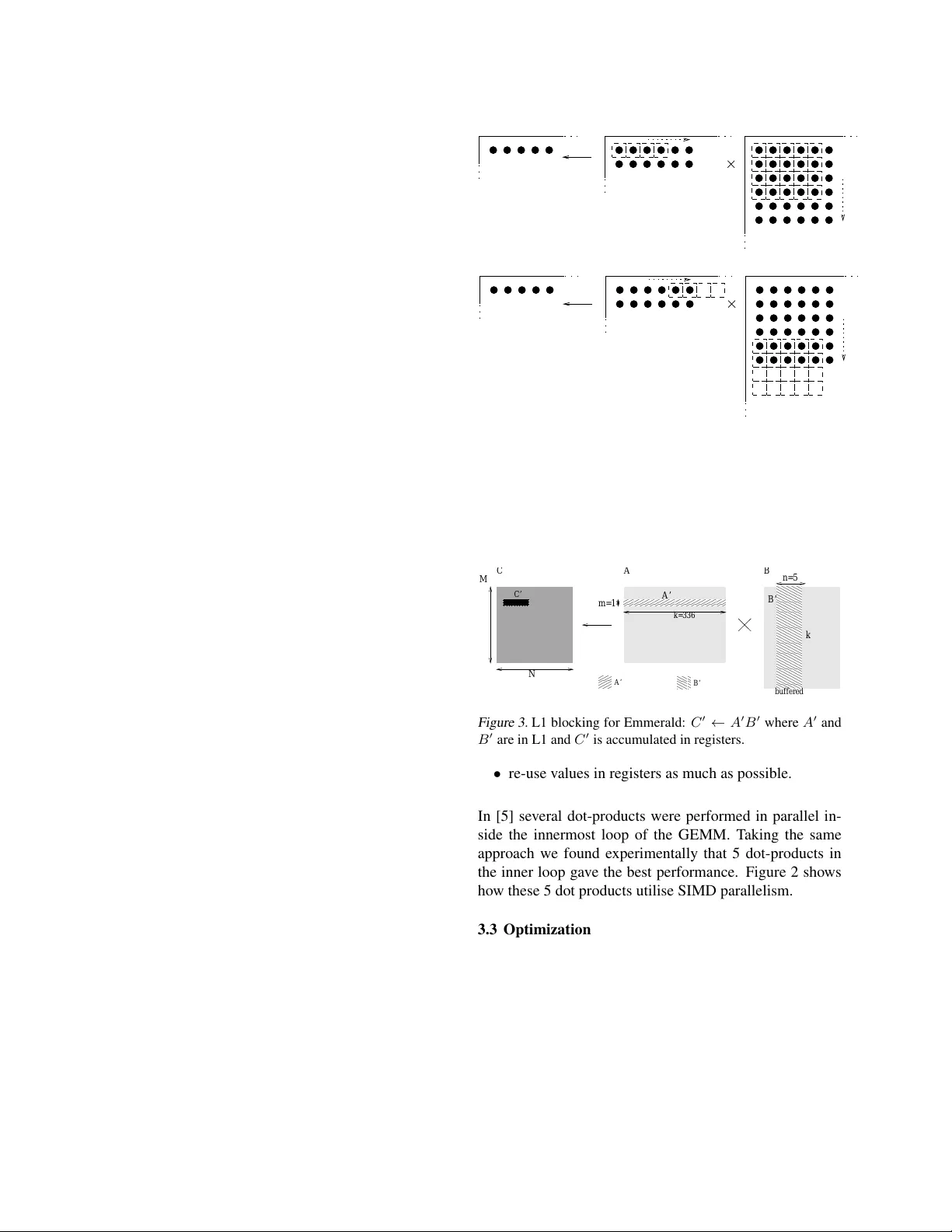
92¢ /MFlops/s, Ultra-Large-Scale Neural-Netw ork T raining on a PIII Cluster Gordon Bell Price/Perf ormance winner . Student paper award finalist Keyw ords: neural-network, Linux cluster , matrix-multiply Douglas Aberdeen (corresponding, pr esenting and student author) D O U G L A S . A B E R D E E N @ A N U . E D U . AU Jonathan Baxter J O NAT H A N . B A X T E R @ A N U . E D U . AU Research School of Information Sciences and Engineering, Australian National Univ ersity , Canberra, Australia, 0200 Robert Edwards R O B E RT . E DWAR D S @ A N U . E D U . AU Department of Computer Science, Australian National Univ ersity , Canberra, Australia, 0200 Abstract Artificial neural networks with millions of ad- justable parameters and a similar number of training e xamples are a potential solution for dif- ficult, large-scale pattern recognition problems in areas such as speech and face recognition, clas- sification of large volumes of web data, and fi- nance. The bottleneck is that neural network training in v olv es iterati ve gradient descent and is extremely computationally intensiv e. In this pa- per we present a technique for distributed train- ing of Ultra Lar ge Scale Neural Networks 1 (UL- SNN) on Bunyip , a Linux-based cluster of 196 Pentium III processors. T o illustrate ULSNN training we describe an experiment in which a neural network with 1.73 million adjustable parameters was trained to recognize machine- printed Japanese characters from a database con- taining 9 million training patterns. The train- ing runs with a av erage performance of 163.3 GFlops/s (single precision). W ith a machine cost of $150,913, this yields a price/performance ratio of 92.4¢ /MFlops/s (single precision). For com- parison purposes, training using double precision and the A TLAS DGEMM produces a sustained performance of 70 MFlops/s or $2.16 / MFlop/s (double precision). 1. Introduction Artificial neural networks are a class of parametric, non- linear statistical models that have found wide-spread use in many pattern recognition domains, including speech recog- nition, character recognition, signal processing, medical di- agnosis and finance. The typical network in such an appli- 1 Follo wing the con vention with integrated circuits, we take ULSNN to mean a neural network with in excess of one million parameters and one million training examples. cation has 100–100,000 adjustable parameters and requires a similar number of training patterns in order to generalize well to unseen test data. Provided suf ficient training data is av ailable, the accuracy of the network is limited only by its representational power , which in turn is essentially pro- portional to the number of adjustable parameters. Thus, in domains where large volumes of data can be collected — such as speech, face and character recognition, and web page classification — improved accuracy can often be ob- tained by training a much larger netw ork. In this paper we describe a method for distributed train- ing of Ultra Larg e Scale Neural Networks (ULSNN), or networks with more than one million adjustable parame- ters and a similar number of training examples. At its core, the algorithm uses Emmerald , a single-precision (32 bit) general matrix-matrix multiply (SGEMM) based on the Pentium III SIMD Streaming Extensions (SSE), with a peak performance in excess of 1090 MFlops/s on a single 550 MHz Pentium III. The use of single-precision floating point operations is justified by the fact that we hav e found it sufficient for gradient-based training of ULSNN’ s. For medium–large scale neural networks as few as 16 bits pre- cision is sufficient [2]. T o illustrate the use of our ULSNN training code, we de- scribe an experiment in which a neural network with 1.73 million adjustable parameters is being trained to recognize machine-printed Japanese characters from a database con- taining 9 million training patterns. The training is run- ning on Bunyip , a 196 processor , Linux-based Intel Pen- tium III cluster consisting of 98 dual 550 MHz processor PC’ s, each containing 384 MBytes of RAM, 13 GBytes of hard disk and 3x100 Mb/s fast Ethernet cards. All components in Bunyip are “COTS” (Commodity-Of f-The- Shelf), and were sourced from a local PC manufacturer (see http://tux.anu.edu.au/Projects/Beowulf/). Our longest experiment took 56 hours and 52 minutes, re- quiring a total of 31 . 2 Peta Flops ( 10 15 single-precision 1 floating-point operations), with an av erage performance of 152 GFlops/s (single precision) while under load. W ith no other user processes running the performance increases to 163.3 GFlops/s which was sustained for a four hour test before returning access to other users. T otal memory usage during training was 32.37 GBytes. The total ma- chine cost, including the labor cost in construction, was A UD$253,000, or USD$150,913 at the exchange rate of A UD$1 = .5965¢ USD on the day of the final and largest payment. This giv es a final price/performance ratio of USD 92.4¢ /MFlops/s (single precision). For comparison purposes, training using double precision and the A TLAS DGEMM [11] produced a sustained performance of 70 MFlops/s or $2.16 /MFlops/s (double precision). 2. “Bunyip” Hardwar e Details The machine used for the experiments in this paper is “Bunyip” , a 98-node, dual Pentium III Beowulf-class sys- tem running Linux kernel 2.2.14. Our main design goals for this machine were to maximise CPU and network per- formance for the giv en budget of A UD $250,000 (about USD $149,125). Secondary factors to be balanced into the equation were: amount of memory and disk; reliability; and the o verall size of the machine. All dollar figures quoted in the remainder of this paper are US dollars. The Intel Pentium III processors were chosen o ver Alpha or SP ARC processors for price/performance reasons. Dual- CPU systems were preferable as overall cost and size per CPU is lo wer than single-CPU or quad-CPU systems. Un- fortunately , at the time of designing this machine AMD Athlon and Motorola/IBM G4 systems were not av ailable in dual-CPU configurations. W e were also keen to use the SSE floating point instructions of the Pentium III range. 550 MHz CPUs were eventually selected as having the best price/performance a v ailable in the Pentium III range at that time. For the networking requirements, we decided to go with a commodity solution rather than a proprietary solution. Gi- gabit ethernet was considered, but deemed too expensi ve at around $300 per node for the NIC and around $1800 per node for the switch. Instead, a novel arrangement of multiple 100 Mb/s NICs was selected with each node hav- ing three NICs which contributed some $65 per node (plus switch costs – see below). The configuration for each node is dual Intel Pentium III 550 CPUs on an EPoX KP6-BS motherboard with 384 MBytes RAM, 13 GByte UDMA66 (IDE) hard disk and three DEC T ulip compatible 100 Mb/s network interfaces, one of which has W ake-On-LAN capability and provision for a Boot R OM. The nodes have no remov able media, no video capability and no keyboards. Each node cost $1282. Giga-Bit Switch Server 2 Server 1 24 Dual PIII, 550 MHz Nodes 48-Port Switches 3 D B C A 1 0 2 4 5 24 x 100Mb/s links Figure 1. Bunyip architecture W ith reference to figure 1, logically the 96 nodes are con- nected in four groups of 24 nodes arranged as a tetrahedron with a group of nodes at each verte x. Each node in a ver- tex has its three NICs assigned to one of the three edges emanating from the verte x. Each pair of vertices is con- nected by a 48-port Hewlett-P ackard Procurve 4000 switch (24 ports connecting each way). The switching capacity of the Procurve switches is 3.8 Gb/s. The bi-sectional band- width of this arrangement can be determined by looking at the bandwidth between two groups of nodes and the other two groups through 4 switches, gi ving a total of 15.2 Gb/s. The 48-port switches cost $2386 each. T wo server machines, more or less identical to the nodes, with the addition of CD-R OM dri v es, video cards and ke y- boards, are each connected to a Netgear 4-port Gigabit switch which is in turn connected to two of the HP Procurve switches via gigabit links. The two server machines also act as connections to the external network. T wo hot-spare nodes were also purchased and are used for dev elopment and diagnostic work when not required as replacements for broken nodes. 2.1 T otal Cost All up we spent 98 x $1282 ($125,636) on the compu- tational nodes (including the two hot-spares), $17,594 on the six 48-port and the 4-port gigabit switches (6 x $2386, 2 x $894 (gigabit interfaces) and $1490 for the gigabit switch), $3870 on servers (including gigabit NICs, moni- tors etc.), $944 for network cables, $179 on electrical w ork, $238 on po wer cables and po wer boards, and $298 on boot EPR OMs. The ex-library shelving was loaned to us, but would hav e cost $354 from a local second-hand furniture shop. Although no component was explicitly budgeted for staff time, this amounted to about 3 weeks to assemble and configure the machine which adds approximately $1800 to the overall cost of the machine. All up, the total cost was USD $150,913. 3. Emmerald: A SIMD SGEMM for Intel Pentium III Pr ocessors This section introduces Emmerald , the high performance software kernel of our ULSNN training system. It pro vides a single-precision, dense, matrix-matrix multiplication rou- tine that uses the single instruction, multiple data (SIMD) features of Intel PIII chips (SIMD Streaming Extensions, or SSE). The SSE provide a set of ne w floating-point assem- bler instructions that allow simultaneous operation on four single-precision floating-point numbers. Emmerald outper - forms a nai ve (3-loop) matrix-matrix multiply by 8 times for square matrices of size 64 , and a peak of 29 times for matrices of size 672 . Emmerald can be downloaded from http://beaker .anu.edu.au/ ∼ daa/research.html. 3.1 Single precision general matrix-matrix multiply (SGEMM) W ithout resorting to the complexities associated with im- plementing Strassen’ s algorithm on deep-memory hierar- chy machines [9, 10], dense matrix-matrix multiplication requires 2 M N K floating point operations where A : M × K and B : K × N define the dimensions of the two ma- trices. Although this complexity is fixed, skillful use of the memory hierarchy can dramatically reduce overheads not directly associated with floating point operations. Memory hierarchy optimization combined with the use of SSE gi v es Emmerald its performance advantage. Emmerald implements the SGEMM interface of Lev el-3 BLAS, and so may be used to improve the performance of single-precision libraries based on BLAS (such as LA- P A CK [8]). There have been several recent attempts at au- tomatic optimization of GEMM for deep-memory hierar- chy machines, most notable are PHiP A C [6] and the more recent A TLAS [11]. A TLAS in particular achiev es per - formance close to vendor optimized commercial GEMMs. Neither A TLAS nor PhiP AC make use if the SSE instruc- tions on the PIII for their implementation of SGEMM. 3.2 SIMD Parallelisation A SIMD GEMM must aim to minimize the ratio of memory accesses to floating point operations. W e employed two core strategies to achie v e this: • accumulate results in registers for as long as possible to reduce write backs; Iteration 2 Iteration 1 4 5 6 7 1 2 1 1 2 1 4 5 6 7 xmm0 xmm3 xmm0 xmm3 xmm1 2 xmm1 2 B C A B A C Figure 2. Allocation of SSE registers (labelled as xmm[0-7] ), showing progression of the dot products which form the inner- most loop of the algorithm. Each black circle represents an ele- ment in the matrix. Each dashed square represents one floating point value in a SSE register . Thus four dotted squares together form one 128-bit SSE register .                                                           buffered k=336 k A’ B’ B A C m=1 M A’ B’ C’ n=5 N Figure 3. L1 blocking for Emmerald: C 0 ← A 0 B 0 where A 0 and B 0 are in L1 and C 0 is accumulated in registers. • re-use values in re gisters as much as possible. In [5] several dot-products were performed in parallel in- side the innermost loop of the GEMM. T aking the same approach we found experimentally that 5 dot-products in the inner loop gav e the best performance. Figure 2 shows how these 5 dot products utilise SIMD parallelism. 3.3 Optimizations A number of techniques are used in Emmerald to improv e performance. Briefly , they include: • L1 blocking : Emmerald uses matrix blocking [5, 6, 11] to ensure the inner loop is operating on data in L1 cache. Figure 3 shows the L1 blocking scheme. The block dimensions m and n are determined by the configuration of dot-products in the inner loop (Sec- tion 3.2) and k was determined e xperimentally . • Unr olling : The innermost loop is completely unrolled for all possible lengths of k in L1 cache blocks, taking care to av oid o verflo wing the instruction cache. • Re-buf fering : Since B 0 (Figure 3) is large (336 × 5) compared to A 0 (1 × 336) , we deliberately buf fer B 0 into L1 cache. While buf fering B 0 we re-order its elements to enforce optimal memory access patterns. This has the additional benefit of minimising transla- tion look-aside buf fer misses [12]. • Pr e-fetching : V alues from A 0 are not buf fered into L1 cache. W e make use of SSE pre-fetch assembler instructions to ensure A 0 values will be in L1 cache when needed. • L2 Blocking : Efficient L2 cache blocking ensures that peak rates can be maintained as long as A , B and C fit into main memory . 3.4 Emmerald Results The performance of Emmerald was measured by timing matrix multiply calls with size M = N = K = 16 up to 700. The following steps were taken to ensure a conser- vati v e performance estimate: • wall clock time on an unloaded machine is used rather than CPU time; • the stride of the matrices, which determines the sepa- ration in memory between each row of matrix data, is fixed to 700 rather than the optimal value (the length of the row); • caches are flushed between calls to sgemm() . T imings were performed on a PIII 450MHz running Linux (kernel 2.2.14). Figure 4 shows Emmerald’ s performance compared to A T - LAS and a naiv e three-loop matrix multiply . The av erage MFlops/s rate of Emmerald after size 100 is 1.69 times the clock rate of the processor and 2.09 times faster than A TLAS. A peak rate of 890 MFlops/s is achieved when m = n = k = str ide = 320 . This represents 1.98 times the clock rate. On a PIII 550 MHz (the processors in Bunyip) we achiev e a peak of 1090 MFlops/s. The lar gest tested size was m = n = k = str ide = 3696 which ran at 940 MFlops/s at 550 MHz. For more detail see [1]. 4. T raining Neural Networks using SGEMM In this section we describe one-hidden-layer artificial neu- ral networks and, following [3], how to compute the gra- dient of a neural network’ s error using matrix-matrix mul- tiplication. W e then describe our conjugate-gradient ap- proach to training neural networks. 0 100 200 300 400 500 600 700 800 900 0 100 200 300 400 500 600 700 Mflops @ 450MHz  Dimension Emmerald Performance Emmerald ATLAS naive Figure 4. Performance of Emmerald on a PIII running at 450MHz compared to A TLAS sgemm and a nai ve 3-loop matrix multiply . Note that A TLAS does not mak e use of the PIII SSE instructions. 4.1 Artificial Neural Networks A one-hidden-layer artificial neural network maps input vectors x = ( x 1 , . . . , x n i ) ∈ R n i to output vectors y = ( y 1 , . . . , y n o ) ∈ R n o according to the formula: y i ( x ) = σ   n h X j =1 w ho ij h j ( x )   , (1) where σ : R → R is some squashing function (we use σ = tanh ), w ho ij are the adjustable parameters connecting the hidden nodes to the output nodes, and h j ( x ) is the acti- vation of the j -th hidden node: h j ( x ) = σ n i X k =1 w ih j k x k ! . (2) In the last expression, w ih j k are the adjustable parameters connecting the input nodes to the nodes in the hidden layer . Giv en a matrix X of n p training patterns and a matrix T of desired outputs for the patterns in X , X =    x 11 . . . x 1 n i . . . . . . . . . x n p 1 . . . x n p n i    , T =    t 11 . . . t 1 n o . . . . . . . . . t n p n o . . . t n p n o    , the goal is to find sets of parameters w ho ij and w ih kl minimiz- ing the mean-squar ed err or : E = n p X i =1 n o X j =1 [ y j ( x i ) − t ij ] 2 , (3) where x i is the i -th ro w of the data matrix X . Usually (3) is minimized by some form of gradient descent. 4.2 Computing The Gradient Using Matrix-Matrix Multiply If we write Y for the matrix of outputs y j ( x i ) , H for the matrix of hidden activ ations h j ( x i ) , and W ih and W ho for the parameter matrices w ih kl and w ho ij respectiv ely , then H = σ  X ∗ W T ih  Y = σ  H ∗ W T ho  where “ ∗ ” denotes ordinary matrix multiplication and σ ( A ) means apply σ elementwize to the components of A . Defin- ing Y ∆ = ( I − Y ∗ ∗ Y ) ∗ ∗ ( T − Y ) , H ∆ = ( I − H ∗ ∗ H ) ∗ ∗ ( Y ∆ ∗ W ho ) , where “ ∗∗ ” denotes elementwize matrix multiplication, we hav e ∇ ih E = H T ∆ ∗ X , ∇ oh E = Y T ∆ ∗ H , where ∇ ih E is the gradient of E with respect to the param- eters W ih and ∇ ho E is the gradient of E with respect to W ho [3]. Thus, computing the gradient of the error for an artifi- cial neural network can be reduced to a series of ordinary matrix multiplications and elementwize matrix multiplica- tions. For large networks and large numbers of training pat- terns, the bottleneck is the ordinary matrix multiplications, which we implement using Emmerald’ s SGEMM routine. In all our experiments we found 32 bits of floating-point precision were enough for training. For neural networks with ≈ 10,000 parameters, as few as 16 bits are suf ficient [2]. Armed with the gradient ∇ E , we can adjust the parame- ters W by a small amount in the ne gati ve gradient direc- tion W := W − α ∇ E and hence reduce the error . How- ev er , because the gradient computation can be very time- consuming (a total of 52.2 T era-floating point operations in our largest experiment), it is more efficient to employ some form of line search to locate a local maximum in the direction ∇ E . For the e xperiments reported in the next sec- tion we used the Polak-Ribiére conjugate-gradient descent method [4, §5.5.2] to choose the search direction, com- bined with an exponential step-size scheme and quadratic interpolation in order to locate a maximum in the search direction. W e were also able to speed the search for a max- imum by using gradient information to bracket the maxi- mum, since only the sign of the inner product of the gradi- ent with the search direction is required to locate the max- imum in that direction, and the sign can be reliably esti- mated with far fewer training patterns than is required to estimate the error . 4.3 T raining Set Parallelism Since the error E and gradient ∇ E are additive over the training e xamples, the simplest way to parallelize the train- ing of a neural network is to partition the training data into disjoint subsets and have each processor compute the error and gradient for its subset. This works particularly well if there are a large number of training patterns so that each processor can work with near-optimal matrix sizes. The communication required is the transmission of the neural network parameters to each sla ve processor, and the trans- mission of the error and gradient information back from each slav e to a master node which reduces them to a single error or gradient vector . 5. Communication This section discusses the communication costs associated with distrib uted NN training, arguing that these costs are non-trivial for ULSNNs. A reduce algorithm optimised for Bunyip’ s topology is also discussed. 5.1 Communication Costs The inter–process communication costs during network training arise from br oadcasting the network parameters to all processes and reducing the network error and gradients from each process to the master process. The parameter broadcasting is cheap, since many copies of the same data is sent to all processes. Broadcasts can take adv antage of features such as TCP/IP broadcasting. The reduce process is more difficult with each process generating unique vec- tors which must be collected and summed by the master process. The time taken to reduce data gro ws with both the number of parameters and the number of processes. The remaining communication consists of start and stop mes- sages which are insignificant compared to the aforemen- tioned costs. A typical neural network with 100 inputs, 50 hidden layer neurons, and 50 output neurons, requires 7500 parameters, or 30 KBytes of data (single precision), to be sent from ev ery node to the master node. A nai ve reduction ov er 194 processes using a 1Gb/s link, such as used in Bunyip, would take 0.05 seconds assuming 100% network utilisa- tion. Our ULSNN with 400 inputs, 480 hidden layer neu- rons and 3203 output neurons requires 1,729,440 parame- ters or 6.6 MBytes of data per process which w ould require 10.1 seconds. There is sufficient memory on each node to occupy both processors for 446 seconds calculating gradi- ents before a reduce operation is required. Consequently the reduce operation would cost at least 2.3% of the av ail- able processing time, more if not enough training data is av ailable or the netw ork size is increased. This demonstrates that although communication costs for distributed NN training are minimal for commonly im- plemented network sizes, ULSNN training must optimise inter–process communication to achie ve the best perfor - mance. W e reduced communication as much as possible by only distributing the neural-network parameters to all the slav es at the very start of training (rather than at each step), and thereafter communicating only the search direction and the amount to step in that direction. One significant reduce op- eration is required per epoch to send the error gradient vec- tor from each process to the master which then co-ordinates the step size search with the slav es. All communication was done using the LAM implementa- tion of MPI (http://www .mpi.nd.edu/lam). Communicat- ing parameters or directions to all processors required a 6.6 MBytes broadcast operation from the server to each of the 194 processors in the cluster , while reducing the gra- dient back to the master required 6.6 MBytes of data to be communicated from each processor back to the server . LAM/MPI contains a library reduce operation which uses a simple O (log n ) algorithm that distributes the load of the reduce o ver many processes instead of naiv ely sending 194 gradient vectors to one node [7]. This results in a reduce operation on Bunyip which takes 8.5 seconds over 8 stages. 5.2 Optimising Reductions There are two problems with e xisting free implementations of MPI reduce operations. The first is the lack of shared memory protocols on clusters with multi-processor nodes, instead using slo w TCP/IP communications between pro- cessors on the same motherboard. Secondly , the reduce operation does not take advantage of the topology of the cluster . For example, the best reduce algorithm to use on a ring network might be to send a single vector to each node on the ring in turn, which adds its contrib ution before pass- ing the vector to the next node. On a star network the best algorithm might be to send each contribution to the central server and sum as the y arri ve. T o decrease the time taken per reduce, we wrote a cus- tomized routine utilising shared memory for intra-node communication and MPI non-blocking calls for inter-node communication. This routine is summarised by Figure 5. It is split into 4 stages, each of which takes adv antage of an aspect of Bunyip’ s topology shown in Figure 1. 1. Each node contains two processors, both running an instance of the training process. All 97 nodes (in- cluding the server), reduce 6.6 MBytes of data though ca da cx dx ba ba aa aa p1 p2 ab bb ax bx 100Mbps ac bc bd ad aa be bu de da du 300Mbps bunyip 1Gbps p1 p2 dx dx 96->48 48->12 12->1 192->96 Figure 5. The four stages of our customized reduce: Stage 1: SHM intra-node reduce; stage 2: all nodes in group A and C reduce to their counterparts; stage 3: groups B and D reduce to 12 nodes using 3 NICs; stage 4: MPI library reduce to the server node. shared memory between processes, taking 0.18 sec- onds. The time taken to add the two sets of data to- gether is approximately 0.005 seconds. 2. Each node in group A can open a 100 Mb/s connec- tion to any node in group B via switch 0. Thus all 24 nodes in A can reduce to their B counterparts in parallel. This requires 0.66 seconds. The same trick is used for reducing from group C to D. The reduced data no w resides only on the B and D nodes. The total bandwidth for all 96 nodes in this stage is 4.03 Gb/s. 3. Each node contains 3x100 Mb/s NICs. This allows a node to receiv e data from three other nodes simultane- ously provided the TCP/IP routing tables are correctly configured. W e split the 24 nodes in each group into 6 sets of 4 nodes. The first of each set (see node B A in Figure 5) is designated as the root and the other three nodes send to it via different NICs. This takes 0.9 seconds achieving a bandwidth of 185 Mb/s into each root node, or 2.22 Gb/s across all 12 root nodes. 4. The final step is a standard MPI library reduce from 6 B nodes and 6 D nodes to the master process. This is the slowest step in the process taking 3.16 seconds, including the time spent waiting for the the nodes to synchronize since they do not start reducing simulta- neously . The overall time taken for the optimised reduce to com- plete is 4.9 seconds. The actual time sav ed per reduction is 3.6 seconds. The training performance speedup from this saving v aries with the duration of the gradient calcula- tion which depends linearly on the number of training pat- terns. Figure 6 illustrates the expected speedup achieved 1 1.1 1.2 1.3 1.4 1.5 1.6 1.7 1.8 1000 10000 100000 1e+06 Speedup  Total training pattens Overall speedup from optimised reduce Figure 6. The overall training performance speedup exhibited af- ter replacing the MPI library reduce with our optimised reduce against the total number of training patters used. by using the optimised reduce instead of the MPI library reduce, against the total number of training patterns used. In practice our peak performance of 163.3 GFlops/s ben- efits by roughly 1% from the optimised reduce, ho we ver the speedups are much more marked for smaller (and more frequently encountered) data sets. 6. Japanese Optical Character Recognition In this section we describe our distributed application of the matrix-matrix multiply technique of Section 3 used to train an artificial neural network as a classifier for machine- printed Japanese characters. 6.1 The Problem, Data and Network Ar chitecture Japanese optical character recognition (Japanese OCR) is the process of automatically recognizing machine-printed Japanese documents and con verting them to an electronic form. The most difficult aspect of Japanese OCR is cor- rectly classifying indi vidual characters, since there are ap- proximately 4000 characters in common usage. The training data for our neural network consisted of 168,000 scanned, se gmented, hand-truthed images of Japanese characters purchased from the CED AR group at the University of Buffalo. The characters were scanned from a variety of sources, including books, faxes, newspa- pers and magazines. Figure 7 gives an idea of the varying quality of the character images. Each character in the CED AR database is represented as a binary image of v arying resolution. W e do wn-sampled all the images to a 20 × 20 grey-scale format. The neural net- work had 400 input nodes, one for each pixel. The database contained examples of 3203 distinct characters, hence the neural-network had 3203 output nodes. The hidden layer Figure 7. Example Japanese characters used to train the neural network. was chosen to have 480 nodes. In total, the network had 1 . 73 million adjustable parameters. 168,000 training examples are not sufficient to avoid ov er- fitting in a network containing 1.73 million adjustable pa- rameters, so we generated synthetic data from the original characters by applying random transformations including line thickening and thinning, shifting, blurring and noise addition. The total number of training examples includ- ing the artificial ones was 9,264,000 approximately 5 . 4 per adjustable network parameter . These were distributed uni- formly to 193 of the processors in Bunyip. A further 6320 examples of the CED AR data set were used for testing pur- poses. 6.2 T raining W ith reference to equations (1), (2), and (3), the total num- ber of floating point operations required to compute the er - ror E in a neural network is 2 × n p × ( n i + n o ) × n h , which equals 32 T era floating-point operations for the Japanese OCR experiment. A gradient calculation uses n p × (4 × n i × n h + 6 × n h × n o ) , or 92 T era floating-point operations. T o assist with load balancing, each slave processor stepped through its training patterns 320 at a time. Between each step the master node w as polled to determine whether more steps were required. Once 80% of the total training data had been consumed, the master instructed all slav es to halt computation and return their results (either the error or the gradient). In this way the idle time spent waiting for other sla ves to finish was reduced to at most the length of time needed by a single processor to process 320 pat- terns. W ith 80% of the data, an error calculation required 26 TFlops and a gradient calculation requires 74 TFlops, or 135 GFlops and 383 GFlops per processor respectiv ely . Patterns % Error 343800 51 611200 46 1833600 33 T able 1. Generalisation error decreases as the total number of pat- terns increases. 7. Results This section describes the classification accurac y achie v ed; then concentrates on the performance scalability over pro- cessors before finishing with peak performance results which result in our claim of a price/performance ratio of 92.4¢ /MFlop/s. 7.1 Classification Accuracy The network’ s best classification error on the held-out 6,320 examples is 33%, indicating substantial progress on a difficult problem (an untrained classifier has an error of 1 − 1 / 3200 = 99 . 97% ). W e observed an error rate of 5% on the 40% of the data which contained the most exam- ples of individual characters. Continued training after the 33% error rate was achie ved improv ed the performance on the common characters at the cost of greatly decreased per - formance on the rare ones. This leads to the conclusion that overfitting is occurring on characters with only one or two examples from the original data set, despite the num- ber of transformations being generated. A more uniform accuracy could be achiev ed by generating more transforms of rare characters, or preferably , using a greater number of original examples. A very large amount of data is required for two reasons. The first is to a void overfitting. T able 1 compares the generalisation accuracy with the total number of training examples used (including transformations of the original 168,000 patterns). Each data point in this graph represents approximately 48 hours training time. T raining was halted after 10 epochs result in no classification improv ement on the test set. 7.2 Communication Perf ormance Recalling from Section 5.1 that communication ov erhead increases with decreasing patterns then the second motiv a- tion for large training sets is to reduce such ov erhead. Fig- ure 8 demonstrates how the performance scales with the number of processors used. The bottom line is the perfor - mance versus processors curve for a small network of 400 input nodes, 80 hidden layer nodes, 200 output nodes and a total of 40,960 training patterns. The middle line is our JOCR ULSNN with 163,480 total patterns. The top line is the JOCR network again, howe v er , for this test we al- lowed the number of patterns to scale with the processors, 0 20 40 60 80 100 120 0 20 40 60 80 100 120 140 GFlops/s  Processors Performance vs processors for large & small problems Large problems Small problems Maximal patterns Figure 8. Performance scaling with the number of processors used for training a small network and our large JOCR network with a fixed number of patterns, and the JOCR problem when the total patterns scales with the number of processors. minimizing the frequency of reduce operations. The max- imal patterns test uses 32,000 patterns per processor . All performance values quoted in this paper represent the to- tal flops that contribute to feed forward value and gradient calculations divided by the wall clock time. Implementa- tion specific flops, such as the reduce operations, were not included. Bunyip w as under a small load during the perfor - mance testing for Figure 8. For a small number of processors, both networks exhibit linear performance scale up, but we observe that for many processors the larger problem scales better despite the in- creased number of network parameters. This is due to the communication overhead in the small network increas- ing dramatically as each processor has less data to process before needing to initiate a reduce. The effect would be clearer for a large network (causing long gradient vectors to be reduced) with fe w training patterns, howe v er this sce- nario is not usually encountered due to overfitting. Finally we observe that with a large enough data set to fill the mem- ory of ev ery node, we achie ve near linear scaling. 7.3 Price/Perf ormance Ratio Bunyip was dedicated to running the JOCR problem for four hours with 9,360,000 patterns distributed across 196 processors. Bunyip actually consists of 194 processors, howe v er , we co-opted one of the hot-spare nodes (included in the quoted price) to make up the other two processors. Over this four hour period a total of 2.35 PFlops were per- formed with an av erage performance of 163.3 GFlops/s. This performance is sustainable indefinitely provided no other processes use the machine. T o calculate the price/performance ratio we use the total cost deri ved in Section 2.1 of USD$150,913, which yields a ratio of 92.4¢ /MFlop/s 2 . 8. Conclusion W e have sho wn how a CO TS (Commodity-Off-The-Shelf) Linux Pentium III cluster costing under $151,000 can be used to achiev e sustained, Ultra-Large-Scale Neural- Network training at a performance in excess of 160 GFlops/s (single precision), for a price/performance ratio of 92.4¢/MFlop/s. Part of the reason for the strong performance is the use of very large training sets. With the current networking set- up, performance degrades significantly with less data per processor , as communication of gradient information starts to dominate ov er the computation of the gradient. Acknowledgements This project was supported by the Australian Research Council, an Australian National Uni versity Major Equip- ment Grant, and LinuxCare Australia. Thanks are also due to several people who made v aluable contributions to the establishment and installation of Bunyip: Peter Christen, Chris Johnson, John Lloyd, Paul McKerras, Peter Strazdins and Andrew T ridgell. References [1] D. Aberdeen and J. Baxter . Ememrald: A fast matrix- matrix multiply using Intel SIMD technology . T echnical report, Research School of Information Science and En- gineering, Australian National Univ ersity , August 1999. http://csl.anu.edu.au/ ∼ daa/files/emmerald.ps. [2] K. Asanovi ´ c and N. Morgan. Experimental determi- nation of precision requirements for back-propagation training of artificial neural networks. T echnical report, The International Computer Science Institute, 1991. ftp://ftp.ICSI.Berkeley .EDU/pub/techreports/1991/tr-91- 036.ps.gz. [3] J. Bilmes, K. Asanovic, C.-W . Chin, and J. Demmel. Us- ing PHiP AC to speed Error Back-Propogation learning. In ICASSP , April 1997. [4] T . L. Fine. F eedforward Neural Network Methodology . Springer , Ne w Y ork, 1999. [5] B. Greer and G. Henry . High performance software on Intel Pentium Pro processors or Micro-Ops to T er - aFLOPS. T echnical report, Intel, August 1997. http:// www .cs.utk.edu/ ∼ ghenry/sc97/paper .htm. [6] J.Bilmes, K.Asanovic, J.Demmel, D.Lam, and C.W .Chin. PHiP AC: A portable, high-performace, ANSI C cod- ing methodoloogy and its application to matrix multiply . 2 Using the exchange rate at the time of writing would yield 91.5¢ USD /MFlops/s, howev er we felt quoting the rate at the time of purchase was a more accurate representation of the cost. T echnical report, Univ ersity of T ennessee, August 1996. http://www .icsi.berkeley .edu/ ∼ bilmes/phipac. [7] LAM T eam. Lam/mpi source code v6.3.2. http://www .mpi.nd.edu/lam/download/. [8] Netlib . Basic Linear Algebr a Subroutines , No vember 1998. http://www .netlib.or g/blas/index.html. [9] V . Strassen. Gaussian elimination is not optimal. Nu- merische Mathematik , 13:354–356, 1969. [10] M. Thottethodi, S. Chatterjee, and A. R. Lebeck. T uning strassen’ s matrix multiplication for memory efficienc y . In Super Computing , 1996. [11] R. C. Whaley and J. J. Dongarra. Automatically tuned linear algebra software. T echnical report, Com- puter Science Department, Uni versity of T ennessee, 1997. http://www .netlib.or g/utk/projects/atlas/. [12] R. C. Whaley , A. Petitet, and J. J. Dongarra. Au- tomated empirical optimizations of software and the atlas project. T echnical report, Dept. of Com- puter Sciences, Univ . of TN, Knoxville, March 2000. http://www .cs.utk.edu/ ∼ rwhaley/A TLAS/atlas.html.