Adaptive Kernel Value Caching for SVM Training

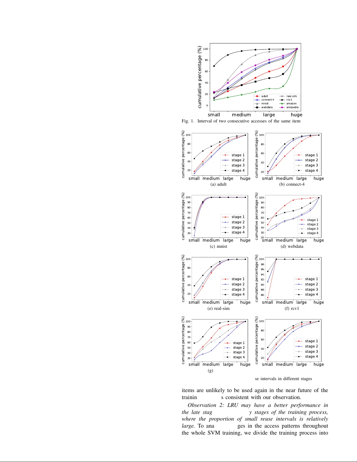
1 Adapti v e K ernel V alue Caching for SVM T raining Qinbin Li, Zeyi W en ∗ , Bingsheng He ∗ Abstract —Support V ector Machines (SVMs) can solve struc- tured multi-output learning problems such as multi-label clas- sification, multiclass classification and vector r egression. SVM training is expensive especially for large and high dimensional datasets. The bottleneck of the SVM training often lies in the kernel value computation. In many real-world problems, the same kernel values are used in many iterations during the training, which makes the caching of kernel values potentially useful. The majority of the existing studies simply adopt the LR U (least recently used) replacement strategy for caching kernel values. However , as we analyze in this paper , the LRU strategy generally achiev es high hit ratio near the final stage of the training, but does not w ork well in the whole training process. Ther ef ore, we pr opose a new caching strategy called EFU (less frequently used) which replaces the less frequently used kernel values that enhances LFU (least frequently used). Our experimental results sho w that EFU often has 20% higher hit ratio than LRU in the training with the Gaussian ker nel. T o further optimize the strategy , we propose a caching strategy called HCST (hybrid caching f or the SVM training), which has a novel mechanism to automatically adapt the better caching strategy in the different stages of the training. W e have integrated the caching strategy into ThunderSVM, a recent SVM library on many-core processors. Our experiments show that HCST adaptively achieves high hit ratios with little runtime overhead among different problems including multi-label classification, multiclass classification and regression problems. Compared with other existing caching strategies, HCST achieves 20% more reduction in training time on av erage. Index T erms —SVMs, caching, ker nel values, efficiency . I . I N T R O D U C T I O N The Support V ector Machine (SVM) [1] is a classic su- pervised machine learning algorithm, and can solve problems with structured, unstructured and semi-structured data [2]. SVMs can solve structured multi-output learning problems, which include multi-label classification [3], [4], [5], multiclass classification [6], [7] and vector regression [8]. Some e xamples applications of SVMs include document classification, object detection, and image classification [9]. The underlying idea of training SVMs is to find a hyperplane to separate the two classes of data in their original data space. T o handle non- linearly separable data, SVMs use a kernel function [10] to map data to a higher dimensional space, where the data may become linearly separable. Although SVMs ha ve several intriguing properties, the high training cost for large datasets is a deficiency . Even though many existing studies hav e been done for accelerating the SVM training [11], [12], [13], the kernel value computation is Q. Li and B. He are with National Univ ersity of Singapore. Email: { qinbin, hebs } @comp.nus.edu.sg Z. W en is with The Univ erisity of W estern Australia. Email: zeyi.wen@uwa.edu.au Z. W en and B. He are the corresponding authors. Digital Object Identifier 10.1109/TNNLS.2019.2944562 c  2019 IEEE usually the most time-consuming operation of the training. T o reduce the cost of k ernel value computation, caching k ernel values may be a good solution. Since the same kernel values are often used in different iterations during the training, we can av oid computing the kernel values if they are cached. Many SVM libraries such as LIBSVM and SVM lig ht [14] adopt the LR U replacement strate gy for caching kernel v alues. LR U works well for occasions with good temporal locality , which may not happen in the SVM training. In order to analyze the patterns in the entire SVM training, we divide the training process into several stages e venly according to the number of iterations. As we observed in the experiments, LRU only works well near the final stage of the training. Howe ver , proposing a suitable caching strategy for the SVM training is challenging, because (i) the access pattern is not trivial to identify , and (ii) the caching strategy should be lightweight in terms of runtime overhead. Based on the pattern analysis, we propose a new strate gy EFU that enhances LFU. The EFU strategy replaces the le ss frequently used kernel values when the cache is full, which is suitable for the access pattern of the kernel values. In order to adapt the access pattern of dif ferent stages, we propose the HCST replacement strategy , which automatically switches to the better strategy between EFU and LRU using the collected statistics. W e collect the exact number of cache hits of the strate gy being used and estimate the approximate number of cache hits of the other strategy based on its characteristic. Thus, HCST can automatically switch the strategy between EFU and LR U. T o reduce the cost of copying data to cache, we perform the replacement of HCST in parallel. Compared with the existing strategies, the HCST strategy can achieve 20% more reduction in training time on average. The main contrib utions of this paper are as follows. • By splitting the training process to stages, we discover common features for the access patterns of dif ferent datasets. • W e propose a ne w caching strate gy , EFU, which enhances LFU to take adv antage of the access patterns of the kernel values. • W e design an adaptiv e caching scheme, HCST , which can fully utilize the characteristics of EFU and LR U to achiev e a better performance. • W e conduct experiments on dif ferent problems includ- ing multi-label classification, multiclass classification and regression problems. The experimental results show that HCST is superior compared with other caching strategies, including LR U, LFU, LA T [15] and EFU. I I . P R E L I M I N A R I E S A N D R E L A T E D W O R K In this section, we first present the formal definition of the SVM training problem, and explain a commonly used SVM 2 training algorithm called SMO . Then, we describe a more re- cent SVM training algorithm [13] which solves multiple SMO subproblems in each iteration and exploits batch processing. Finally , we discuss the existing SVM libraries and caching strategies. A. The SVM training pr oblem A training instance x i is attached with an integer y i ∈ { +1 , − 1 } as its label. A positive (negati ve) instance is an instance with the label of +1 ( − 1 ). Giv en a set χ of n training instances, the goal of the SVM training is to find a hyperplane that separates the positive and the negati ve training instances in the feature space induced by the kernel function with the maximum margin and meanwhile, with the minimum misclassification error on the training instances. The SVM training is equi v alent to solving the following problem: max α n X i =1 α i − 1 2 α T Qα subject to 0 ≤ α i ≤ C, ∀ i ∈ { 1 , ..., n } , n X i =1 y i α i = 0 (1) where α ∈ R n is a weight vector , and α i denotes the weight of x i ; C is for regularization; Q denotes an n × n matrix and Q = [ Q ij ] , Q ij = y i y j K ( x i , x j ) and K ( x i , x j ) is a kernel value computed from a kernel function. Kernel functions (e.g., the Gaussian k ernel function [10], the ideal kernel function [16]) are used to map the problem from the original data space to a higher dimensional data space. F or a training set with n instances, the i th row K i = h K ( x i , x 1 ) , K ( x i , x 2 ) , ..., K ( x i , x n ) i of the k ernel matrix corresponds to all the n kernel values of the instance x i . B. The SMO algorithm Problem (1) is a quadratic programming problem, and can be solved by many algorithms. Here, we describe a popular training algorithm, namely the Sequential Minimal Optimization (SMO) algorithm [11], which is adopted in many existing SVM libraries such as LIBSVM [17] and liquidSVM [18]. The SMO algorithm iterativ ely improves the weight vector α until the optimal condition of the SVM is met. The optimal condition is reflected by an optimality indicator vector f = h f 1 , f 2 , ..., f n i where f i is the optimality indicator for the i th instance x i and f i can be obtained using the following equation: f i = P n j =1 α j y j K ( x i , x j ) − y i . The SMO algorithm has the following three steps: Step 1 : Find two extreme training instances, denoted by x u and x l , which hav e the minimum and maximum optimality indicators, respecti vely . The indexes of x u and x l , denoted by u and l respectively , can be computed by the follo wing equations [19]. u = argmin i { f i | x i ∈ X upper } l = argmax i { ( f u − f i ) 2 η i | f u < f i , x i ∈ X lower } (2) where X upper = X 1 ∪ X 2 ∪ X 3 , X lower = X 1 ∪ X 4 ∪ X 5 and X 1 = { x i | x i ∈ X , 0 < α i < C } X 2 = { x i | x i ∈ X , y i = +1 , α i = 0 } X 3 = { x i | x i ∈ X , y i = − 1 , α i = C } X 4 = { x i | x i ∈ X , y i = +1 , α i = C } X 5 = { x i | x i ∈ X , y i = − 1 , α i = 0 } η i = K ( x u , x u ) + K ( x i , x i ) − 2 K ( x u , x i ) f u and f l denote the optimality indicators of x u and x l , respectiv ely . Step 2 : Improve the weights of x u and x l , denoted by α u and α l , by updating them as follows. α 0 l = α l + y l ( f u − f l ) η , α 0 u = α u + y l y u ( α l − α 0 l ) where η = K ( x u , x u )+ K ( x l , x l ) − 2 K ( x u , x l ) . T o guarantee the update is v alid, when α 0 u or α 0 l exceeds the domain of [0 , C ] , α 0 u and α 0 l are adjusted into the domain. Step 3 : Update the optimality indicators of all the training instances. The optimality indicator f i of the instance x i is updated to f 0 i using the follo wing formula: f 0 i = f i + ( α 0 u − α u ) y u K ( x u , x i ) + ( α 0 l − α l ) y l K ( x l , x i ) SMO repeats the above steps until the follo wing condition is met. f u ≥ f max = max { f i | x i ∈ X lower } (3) C. A mor e recent SVM training algorithm based on SMO As we hav e mentioned in Section II-B, the SMO algorithm selects two training instances (which together form a w orking set) to improv e the current SVM. Instead of using a working set of size two, a more recent SVM training algorithm uses a bigger working set and solves multiple subproblems of SMO in a batch [13], which is implemented in ThunderSVM 1 . Giv en the training dataset, ThunderSVM does the follo wing steps to train the SVM. First, a w orking set is formed with a number of instances that violate the optimality condition the most. Second, the ro ws of kernel values needed for the subproblems corresponding to the working set are computed. Third, the SMO algorithm is used to solve each of the subproblems. ThunderSVM repeats the above steps until the termination criterion is met. The second step can be done by matrix multiplication, and the third step can be solved by SMO as discussed in Sec- tion II-B. Solving the first step is much more challenging. Here we elaborate the details about the first step. At each iteration when ThunderSVM updates the working set, q instances in the working set will be replaced with q new violating instances (e.g., q = 512 by default in ThunderSVM). The intuition for updating the working set is to choose q training instances 1 For ease of presentation, we use ThunderSVM to refer to “the SVM training algorithm implemented in ThunderSVM”. 3 that violate the optimality condition (cf. Inequality 3) the most, such that the current SVM can be potentially improv ed the most. ThunderSVM does not update the whole w orking set to mitigate the local optimization. ThunderSVM sorts the optimality indicators ascendingly . Then, it chooses the top q / 2 training instances whose y i α i can be increased, and the bottom q / 2 training instances whose y i α i can be decreased. Thunder- SVM considers y i α i , because of the constraints 0 ≤ α i ≤ C and P n i =1 y i α i = 0 in Problem (1). In summary , the training algorithm of ThunderSVM has two phases: selecting a working set from the training dataset, and solving the subproblems using SMO. Since the same ro w of the kernel v alues is often used multiple times in different iterations during the training, we can adopt a cache to store the kernel values to reuse them between the iterations. D. Existing SVM libraries and caching One of the key factors for the success of SVMs is that many easy-to-use libraries are a vailable. The popular libraries include SVM lig ht [20], LIBSVM [17] and ThunderSVM. SVM lig ht , LIBSVM and many other SVM libraries (e.g., liquidSVM) adopt the LR U strategy for kernel value caching, while ThunderSVM has not applied caching strategy . The LR U caching strate gy works well for occasions with good temporal locality . Ho we ver , no evidence has shown that the time of the reuse interval of kernel v alues is relati vely small, and hence the LRU caching strate gy may not be a good option for kernel value caching in the SVM training. MASCO T [15] adopts a new caching strategy called LA T . When the cache is full, LA T replaces the row with the minimum ro w index in the kernel matrix. LA T effecti vely caches the last part of the kernel matrix which is stored in SSDs in MASCO T . This mak es LA T prefer to cache kernel values stored in SSDs rather than those in the main memory . LA T shows better performance than LRU on MASCO T . I I I . M O T I V A T I O N S For ease of presentation, we call one ro w of k ernel matrix an item , which is the smallest unit for the replacement operation in the training. Our design of HCST is motiv ated by the following observations of the access pattern of the items. Observation 1: Due to the r elatively larg e reuse interval, LR U is not suitable for the overall training. Suppose the cache can store at most 5,000 items. W e define r euse interval R to be the number of iterations between two consecuti ve accesses to an item. For clarity of presentation, we di vide the reuse interval R to four dif ferent le vels: small ( 0 < R < 5 , 000 ), medium ( 5 , 000 ≤ R < 10 , 000 ) , larg e ( 10 , 000 ≤ R < 15 , 000 ) and huge ( R ≥ 15 , 000 ). Figure 1 shows the cumulati ve percentage of dif ferent le vels. LRU works well if most reuse interv als are small so that the item is still in cache when accessed again. Howe ver , as we can see from the results, except for rcv1 , the proportion of small reuse interv al is very low , which means LR U is not a suitable strategy for the kernel v alue caching in SVM training. W en et al . [15] has prov ed that the items are accessed in a quasi-round-robin manner , where the selected small medium large huge 0 20 40 60 80 100 cumulative percentage (%) adult connect-4 mnist webdata real-sim rcv1 amazon wikipedia Fig. 1. Interval of two consecutive accesses of the same item small medium large huge 20 40 60 80 100 cumulative percentage (%) stage 1 stage 2 stage 3 stage 4 (a) adult small medium large huge 20 40 60 80 100 cumulative percentage (%) stage 1 stage 2 stage 3 stage 4 (b) connect-4 small medium large huge 30 40 50 60 70 80 90 100 cumulative percentage (%) stage 1 stage 2 stage 3 stage 4 (c) mnist small medium large huge 20 30 40 50 60 70 80 90 100 cumulative percentage (%) stage 1 stage 2 stage 3 stage 4 (d) webdata small medium large huge 20 40 60 80 100 cumulative percentage (%) stage 1 stage 2 stage 3 stage 4 (e) real-sim small medium large huge 86 88 90 92 94 96 98 100 cumulative percentage (%) stage 1 stage 2 stage 3 stage 4 (f) rcv1 small medium large huge 30 40 50 60 70 80 90 100 cumulative percentage (%) stage 1 stage 2 stage 3 stage 4 (g) amazon small medium large huge 20 40 60 80 100 cumulative percentage (%) stage 1 stage 2 stage 3 stage 4 (h) wikipedia Fig. 2. Cumulativ e distribution of reuse intervals in different stages items are unlikely to be used again in the near future of the training, which is consistent with our observation. Observation 2: LR U may have a better performance in the late stag e than the early stag es of the training pr ocess, wher e the pr oportion of small r euse intervals is r elatively lar ge. T o analyze changes in the access patterns throughout the whole SVM training, we divide the training process into 4 0 1 2 >=3 0 20 40 60 percentage (%) stage 1-2 stage 2-3 stage 3-4 (a) adult 0 1 2 >=3 0 20 40 60 80 percentage (%) stage 1-2 stage 2-3 stage 3-4 (b) connect-4 0 1 2 >=3 0 20 40 60 percentage (%) stage 1-2 stage 2-3 stage 3-4 (c) mnist 0 1 2 >=3 0 20 40 60 80 percentage (%) stage 1-2 stage 2-3 stage 3-4 (d) webdata 0 1 2 >=3 0 20 40 60 80 percentage (%) stage 1-2 stage 2-3 stage 3-4 (e) real-sim 0 1 2 >=3 0 20 40 60 80 percentage (%) stage 1-2 stage 2-3 stage 3-4 (f) rcv1 0 1 2 >=3 0 20 40 60 80 percentage (%) stage 1-2 stage 2-3 stage 3-4 (g) amazon 0 1 2 >=3 0 20 40 60 80 percentage (%) stage 1-2 stage 2-3 stage 3-4 (h) wikipedia Fig. 3. Distribution of the difference of access frequencies in different stages four stages ev enly according to the number of iterations. W e ha ve also tested different number of stages such as two and eight, and observed similar results. Figure 2 sho ws the cumulativ e distribution of reuse intervals in different stages. W e observe that there are some common features of the access patterns in the training progress. The stage 4 always has the highest proportion of small reuse intervals. Here is a scientific explanation. Compared with the early stages, the SVM training is more likely to choose the support vectors to adjust the hyperplane near the end of the training process [21]. Then, the distribution of the accesses is more concentrated in the late stage. Thus, the proportion of small reuse interval is larger in the late stage, where LR U may hav e a good performance. So LR U can perform better in the late stage of the training. Observation 3: The items tend to have similar access fre- quency acr oss differ ent stages. In order to study the uniformity of access frequencies of the items, we calculate the dif ference of access frequencies of the same item between different stages. The distribution of the dif ference are sho wn in Figure 3. W e can find the distrib ution of access frequencies is quite uniform in different stages. More than 60% of the items hav e no difference in the access frequencies of different stages. This observation results from the property of the SVM training. In many real world problems, most training instances are non- support vectors, which are not actively selected to update the hyperplane in the whole training process [20]. Then, for most items, the access frequencies across different stages tend to be low and close. Based on this characteristic, items with higher access frequency should be cached since they are likely to be accessed with a higher frequenc y in the subsequent training progress. A classic algorithm for frequenc y based cache re- placement is LFU. Howe ver , the LFU strategy always caches the ne wly generated item and replaces the least frequently used item in cache, e ven though the item in cache has a higher frequency than the ne w item, which is not good enough for caching items with higher access frequencies. That is why we propose to enhance LFU with EFU. I V . T H E H C S T S T R A T E G Y A. An Overview of HCST The structure of the SVM training with HCST is shown in Figure 4. There are mainly two components of HCST : the candidate strategies and the strategy selection. In the iterativ e process of the SVM training, HCST selects the better caching strategy from candidate strategies and applies it until the next selection. The main aim of HCST is to improve the hit ratio of items in the entire training process. 1) Candidate strate gies: According to the observations in Section III, we use EFU and LRU as our candidate strategies. EFU is our proposed caching strategy , which aims to cache the items with higher access frequencies. W e will introduce the details of EFU in Section IV -B. LR U is a classic caching strategy , which aims to cache the items with recently time used. By splitting the training process to different stages, as we claimed in Section III, we ha ve two key findings. One is that the items with higher access frequency are more likely to also be accessed more times in the next stage, which is fully utilized by EFU. The other one is that the reuse interval of items is likely to be smaller in the late stage of the training process, which makes LR U a potentially suitable strategy . By making full use of these two features, we propose the EFU strategy and use it and LR U as our candidate strategies. 2) Strate gy selection: At first we adopt the EFU strategy , which appears to have a good performance in the overall training. During the training, after ev ery fixed number of iterations, we make a selection from the candidate strategies based on collected statistics. Here we use the number of cache hits as the criterion. If the number of cache hits of EFU is bigger than that of LR U in the current stage, we adopt EFU in the next stage, otherwise we adopt LR U. In this way we can switch to LR U timely if LRU already works better than EFU. In addition, due to the jitter of the number of hits using LR U, there are some cases we switch to LR U prematurely . This deficienc y is generally fine, since HCST can switch back to EFU quickly in the next comparisons. In general, HCST is pure EFU if no switch happens or piecewise EFU and LRU if any switch happens in the training process. 5 Candidate Strategies EFU LRU Strategy Selection Iteratively T raining Maintaining Cache Fig. 4. The process of the SVM training with HCST M 4 5 cache access counts of items newly computed items M 1 M 2 M 3 4 5 4 cache M 4 M 2 M 3 5 5 4 M 5 2 cache M 4 M 2 M 3 5 5 4 Fig. 5. A running example of EFU B. The EFU strate gy The key ideas of EFU are described as follo ws. W e maintain a counter for each item of the kernel matrix to record the access frequency . When a new item is computed and the cache is already full, we first decide whether it will be added into the cache. If all the items in the cache have higher accumulated access frequencies than the new item, EFU will not cache it. Otherwise, EFU replaces the item in the cache with a lower access frequency than this ne wly computed item. In this way , we can alw ays store the items which ha ve higher frequenc y of usage currently in the SVM training. Figure 5 shows a running example of EFU. Suppose the cache stores 3 items: M 1 , M 2 and M 3 . These items hav e been accessed 4 times, 5 times and 4 times, respectiv ely . When a ne wly computed item M 4 comes, EFU finds the item M 1 which has a lo wer access frequency than M 4 and replaces it. When another newly computed item M 5 comes, EFU does not do replacement since no item in the cache has a lower access frequency . The LFU strategy alw ays replaces the least frequently used item, e ven though it has a higher access frequenc y than the new item, while the EFU strategy can a void the problem. EFU is more suitable to store the items with higher access frequencies compared with LFU. C. The HCST strate gy As we hav e shown in Figure 2, the proportion of small reuse distance differs clearly in the late stage of the training process. There may be some cases where the performance of LRU is better than EFU in the late stages as the training processes. T o handle it, we implement a dynamic strategy called HCST which allows the caching strategy to switch between EFU and LR U. At the beginning of training, we adopt EFU. In regular stages during the training, we compare the number of cache hits if adopted LR U ( H LRU ) with the number of cache hits if adopted EFU ( H E F U ). If we found H LRU is bigger than H E F U , we use LR U for the next stage, otherwise using EFU. As we ha ve discussed in Section III, the performance of LR U strategy can be better in the late stage of the SVM training, so it is reasonable to switch the strategy to LR U if the hit number of LR U is already bigger than EFU. Furthermore, to reduce the bad ef fect of the premature switching from EFU to LR U, which may be caused by the instability of the number of cache hits using LR U, HCST can switch back to EFU timely in the next comparison. In practice, it is challenging to know the exact number of cache hits of both strategies since we only can adopt one strategy at one time. Ho we ver , we can estimate the number of cache hits based on the features of the cache strategy . For ease of presentation, we call the time we compare H LRU with H E F U as a checkpoint. Suppose the cache size is s which means at most s items can be cached. Assume we are using EFU before a checkpoint T 1 . W e use a counter to record the number of cache hits H hit after T 1 . So H hit is the e xact H E F U when we arri ved the ne xt checkpoint T 2 . W e use another counter to record the number of accesses H s whose reuse interval is smaller than s after T 1 . Note that these accesses can all yield cache hits if using LR U. So we use H s as the approximate H LRU when we arriv ed T 2 . If H s is not bigger than H hit in T 2 , we do not change the strategy and do the same operations for the next stage. If H s is bigger than H hit , we change the strategy to LR U and sav e the value H hit . When using LR U, we still use the counter to record the number of cache hits H hit 0 after checkpoint T 2 , which is the exact H LRU . Since the distri- bution of access frequencies is quite e venly as we describe in Section III, the hit ratio of EFU should be close between different stages. So we use H hit as the approximate H E F U . In the ne xt checkpoint T 3 , we compare H hit 0 with H hit . If H hit 0 is smaller than H hit , we switch the strategy back to EFU. Otherwise we do not change the strategy . Algorithm 1 shows the training process with the HCST strategy . Overall, we can get the exact number of cache hits with the strategy being used and estimate the approximate number of cache hits if adopted the other strategy . By comparing these two values, the dynamic selection of the strategies can make efficient use of the characteristics we observed for the access patterns of the items. D. Optimization for multi-output learning tasks By adopting the “one-vs-all” scheme, we can transform a multi-output learning task into a set of independent single- output learning tasks [6]. Then. we train a solver for each single-output learning task. Since each solver can utilize the CPU resources well, the solvers are trained in a sequential manner . Although the training of each solver is independent, they use the same training instances. T o exploit this property , we can reuse the kernel v alues between different solvers. Instead of adopting individual cache for each solver , we use one shared cache during the whole training process for the multi-output tasks. Thus, after a solver finishes the training, the kernel values in the cache can still be reused in the next solver . In summary , there are two le vels of reuses of the kernel values in the multi-output learning tasks. One is the reuse 6 Algorithm 1: Pseudo of the training process with HCST Input: The training dataset Output: The SVM model 1 Adopt EFU at the beginning; 2 while the optimality condition of SMO is not met do 3 if is a checkpoint then 4 if is using EFU then 5 Get the number of cache hits with EFU ( H hit ); 6 Estimate the number of cache hits with LR U ( H s ); 7 if H hit < H s then 8 Sav e the value H hit ; 9 Switch to LR U; 10 else 11 Get the number of cache hits with LR U ( H hit 0 ); 12 Estimate the number of cache hits with EFU ( H hit ); 13 if H hit 0 < H hit then 14 Switch to EFU; 15 T raining; of the kernel values between different iterations of a solver (iteration-lev el reuse). The other one is the reuse of the kernel values between different solvers of the training process (solv er - lev el reuse). Compared with the original HCST , which only exploits the iteration-le vel reuse, the solver -le vel reuse can fully utilize the characteristic of the multi-output learning task and has no e xtra ov erhead. As we will sho w in Section V -C4, our technique can reduce the training time significantly . E. P ar allel implementation of the replacement operations Since ThunderSVM accesses q items on each iteration, it is time-consuming to do replacement one by one. T o reduce the cost of caching, we implement the parallel replacement operation, which is sho wn in Figure 6. Suppose we have p threads and there are u items that yield cache misses among accessed q items. W e e venly di vide these u items into p groups, and each group is assigned to one thread. T o av oid conflicts in the cache when multiple threads perform the replacement, we also divide the cache into p parts, and each part is assigned to one thread. Each thread traverses its corresponding part to find an eligible item to replace. Since each thread performs replacement operations for the same number of items (i.e., u/p ) and has the same size of cache space (i.e., s/p ) to trav erse, the workload of each thread is balanced. By using multiple threads, we can reduce the cost of the replacement significantly , as we will show in Section V -C. F . Efficiency analysis Here we analyze the theoretical efficienc y of the HCST strategy . W e suppose the cardinality of the dataset is n and cache · · · thread 1 thread p do replac ement do replac ement ac c essed items that yield cache misses · · · · · · M k M k+1 M k+s-s/p M i M i+1 M i+u/p-1 M i+u-1 M k+s/p-1 · · · · · · M k+s-2 M k+s-1 M i+u-u/p · · · M i+u-2 · · · · · · Fig. 6. The parallel replacement operations the dimension of the dataset is d . ThunderSVM accesses q items on each iteration. 1) T ime complexity of the r eplacement: Suppose the cache size is s . W e need at most O ( s ) to trav erse on the cache to find an item that meets the requirements of the cache strategy to replace. On each iteration, there are at most q items to be replaced. So the time comple xity of our caching strategy in one iteration is O ( q s ) . T ime complexity impr ovement by parallelism : Suppose the number of threads is p . If we perform the replacement in parallel, we only need O ( s/p ) to find an item to replace. Additionally , each thread only needs to handle at most q/p items. The time complexity of HCST in one iteration is O ( qs/p 2 ) , which is reduced by p 2 times compared with performing replacement in serial. This property makes HCST appealing in the context of parallel computing. Overhead of the dynamic selection : Although the HCST strategy needs a selection operation in the training process, the cost of it is very low . T o get the hit number of EFU and LR U, we need maintain counters for each item as we ha ve discussed in Section IV -C. W e need O ( q ) to update these counters in each iteration, where q is much smaller than n . The comparison between the numbers of cache hits can be done in O (1) . The ov erhead of the dynamic selection is O ( q ) in each iteration, which can be ignored compared with the time complexity of the training. 2) Memory consumption of the HCST strate gy: T o enable the switch between EFU and LR U, we need maintain two counters for each item to record the access frequency and the recently used time. Suppose each integer and float use 4 bytes to store. So we need 8 n bytes for all counters. The extra cost of memory is very small compared with the size of the dataset, which costs 4 nd bytes to store. 3) Benefit of caching: W e can compute the benefit of caching theoretically for the SVM training. Suppose the num- ber of floating point operations per second (i.e., flops) of CPU is l . Suppose we use the Gaussian kernel for the SVM training. The Gaussian kernel is defined as follows. K ( x i , x j ) = exp {− γ ( || x i || 2 + || x j || 2 − 2 x T i x j ) } T o compute an item (i.e., a ro w of the kernel matrix), we need to compute the inner products of all the n training 7 instances (i.e., n v ectors of 1 × d dimensions), a multiplication of a 1 × d vector and a d × n matrix (i.e., x i and the whole training dataset). Hunger [22] sho wed the flops of the dot product computation is (2 d − 1) n . Since inner products are computed only once at the beginning of the SVM training, we do not count them in the cost. Ignoring the floating operations to compute the exponential formula, we can get the cost for computing an item as T o = (2 d − 1) n/l . Suppose the number of cache hits is h . The time of kernel value computation sa ved by the caching strategy T s = h (2 d − 1) n/l . Let the number of replacement operations be u . T o simplify the model, we assume the sequential copy bandwidth of memory is a constant b . Each kernel v alue is 4 bytes. The size of an item is 4 n bytes. So we can compute the time of replacement in cache as T c = 4 un/b . Ignoring other costs, we can get the benefit of caching strategy as follows. T b = T s − T c = h (2 d − 1) n/l − 4 un/b (4) Equation (4) shows the benefit is positi vely related to the number of hits and negati vely related to the number of copies. Furthermore, for datasets with higher cardinality and dimensionality , the benefit is higher . V . E X P E R I M E N T A L S T U D Y In this section, we present the empirically results of our proposed caching strategy HCST . W e conducted the experi- ments on a workstation running Linux with two Xeon E5- 2640v4 10 core CPUs and 256GB main memory . The number of threads is set to 20 by default to effecti vely utilize the resources of CPUs. The maximum number of items that cache can store is set to 5,000 by default, which is a relativ ely small size with little memory cost. W e also try different cache sizes (i.e., 10K, 15K and 20K) in our experiments. The number of iterations between two consequent checkpoints is set to 20, which is an appropriate v alue as we will sho w in Section V -C1. The cache replacement strate gies we used in our experiments include HCST , LR U, EFU, LFU and LA T . T o ensure f airness, we used the same data structure to implement all the cache strategies. The kernel functions we used in our experiments include the Gaussian kernel and the sigmoid kernel. W e used ThunderSVM as our training library and the stopping criteria are the same for all the experiments. W e used 14 public datasets from the LIBSVM website 2 and this link 3 with four dif ferent problems including binary , multi- label and multiclass classification, and regression. Among 14 datasets, 6 datasets ( adult , connect-4 , mnist , webdata , r eal- sim and rcv1 ) are used in every experiment while the other 8 datasets are used together with the previous datasets to more thoroughly ev aluate the training time of SVMs with HCST . For mediamill and rcv1s2 , the label dimensionality is 101. For amazon and wikipedia , we randomly choose 10 labels to perform the classification task. T able I gives the details of the datasets and parameters of kernel functions used in the experiments. The parameters are the same as the existing 2 https://www .csie.ntu.edu.tw/ ∼ cjlin/libsvm/index.html 3 http://manikvarma.or g/do wnloads/XC/XMLRepository .html T ABLE I DAT A S E T S A N D K E RN E L PA R AM E T E RS dataset task cardinality dimension Gaussian sigmoid C γ C γ adult binary classification 32,561 123 100 0.5 10 0.01 rcv1 20,242 47,236 100 0.125 10 0.5 real-sim 72,309 20,958 4 0.5 10 0.5 webdata 49,749 300 10 0.5 10 0.01 covtype 581,012 54 3 1 10 0.5 connect-4 multiclass classification 67,557 126 1 0.3 10 0.001 mnist 60,000 780 10 0.125 10 0.001 mnist8m 8,100,000 784 1000 0.006 mediamill multi-label classification 30,993 12,914 10 0.5 10 0.01 rcv1s2 3,000 101 10 0.5 10 0.5 amazon 1,717,899 337,067 10 0.5 10 0.5 wikipedia 1,813,391 2,381,304 10 0.5 10 0.5 abalone regression 4,177 8 10 0.5 10 0.01 E2006-tfidf 16,087 150,360 10 0.5 10 0.01 adult connect-4 mnist webdata real-sim rcv1 0 20 40 60 80 100 hit ratio (%) with Gaussian kernel HCST LRU LFU LAT EFU (a) Hit ratio with the Gaussian k ernel adult connect-4 mnist webdata real-sim rcv1 0 20 40 60 80 100 hit ratio (%) with sigmoid kernel HCST LRU LFU LAT EFU (b) Hit ratio with the sigmoid k ernel Fig. 7. Hit ratio comparison 5K 10K 15K 20K cache size 10 20 30 40 50 60 70 80 hit ratio (%) HCST LFU LRU LAT EFU (a) adult 5K 10K 15K 20K cache size 10 20 30 40 50 60 hit ratio (%) HCST LFU LRU LAT EFU (b) connect-4 5K 10K 15K 20K cache size 20 30 40 50 60 70 hit ratio (%) HCST LFU LRU LAT EFU (c) mnist 5K 10K 15K 20K cache size 20 30 40 50 60 hit ratio (%) HCST LFU LRU LAT EFU (d) webdata 5K 10K 15K 20K cache size 10 20 30 40 50 60 70 80 hit ratio (%) HCST LFU LRU LAT EFU (e) real-sim 5K 10K 15K 20K cache size 50 55 60 65 70 75 80 85 90 hit ratio (%) HCST LFU LRU LAT EFU (f) rcv1 Fig. 8. Hit ratio with dif ferent cache sizes study [15], [23], [24] or selected by a grid search ( C ranges from 1 to 10 and γ ranges from 0.001 to 0.5). 8 A. Hit ratio comparison K ey finding 1: HCST can always achie ve the highest hit ratio among all the caching strate gies. Figure 7 shows the hit ratio of different caching strategies. W e tried two dif ferent kernel functions: the Gaussian kernel and the sigmoid kernel. W e first compare the four caching strategies except HCST . EFU and LFU have a relativ ely better performance when using the Gaussian kernel, while LR U outperforms the other strategies when using the sigmoid kernel. Furthermore, the hit ratio of EFU is higher than LFU on some datasets with the Gaussian kernel (e.g., adult and mnist ). The LA T strategy does not sho w adv antage on both two kernel functions. Except for HCST , none of the strategies is optimal across dif ferent datasets and dif ferent kernel functions. Howe ver , due to our specialized design, HCST is comparable to or even better than the best of them in all cases. HCST can adaptiv ely achieve high hit ratios among dif ferent cases. Figure 8 shows the hit ratio of different caching strategies with dif ferent cache sizes using the Gaussian k ernel, which is the most widely used kernel function in the SVM training. The HCST strategy alw ays has good performance on different settings of cache size in the e xperiments. Furthermore, all five cache replacement strategies hav e a similar hit ratio when the cache size is big. This is because when the cache is large enough, the cache can store almost all the items. As a result, the accesses that yield cache misses are mainly first usages of the items, which are inevitable no matter what caching strategy is used. Note that the increase in memory size can not keep up with the speed of data growth. The memory size is al ways relatively small compared with the size of kernel values of huge datasets. The HCST strategy is superior to the other strategies when the memory for cache is limited. B. The overall training with HCST K ey finding 2: HCST can always clearly reduce the SVM training time. T o show the performance of the HCST strategy , we compare it with the cache strate gies LR U, LFU, LA T and EFU on all the 14 datasets. In T able II, we show the elapsed training time of no cache and the relati ve values of the other caching strategies against no cache. Compared with HCST , the other strategies hav e a smaller improv ement, and sometimes even have no benefit due to the cost of caching (e.g., adult ). The HCST strategy has a stable improv ement and helps improve the SVM training without caching by at least 25% in all 14 datasets. For r cv1 , the speedup is bigger than 4. For the multi-label datasets, HCST can reduce the training time by at least 30%, which is a significant improv ement. T able III sho ws the calculation time of k ernel values and the cost of caching when using dif ferent caching strategies with the Gaussian kernel. Compared with LFU, LR U, LA T and EFU, HCST al ways has lo wer calculation time of k ernel v alues and lower cost of caching. As we have sho wn in Figure 7a, the HCST strategy mostly has a higher hit ratio than the other strategies, especially LR U and LA T , which explains the lo wer calculation time of kernel v alues. As we ha ve discussed in 70 80 90 0.5 1 2 4 8 20 30 40 hit ratio (%) adult connect-4 mnist webdata real-sim rcv1 (a) Gaussian kernel 80 100 0.5 1 2 4 8 30 40 50 hit ratio (%) adult connect-4 mnist webdata real-sim rcv1 (b) sigmoid kernel Fig. 9. Hit ratio with dif ferent λ 0.5 1 2 4 8 0 1 2 number of switches adult connect-4 mnist webdata real-sim rcv1 (a) Gaussian kernel 0.5 1 2 4 8 0 2 4 6 8 number of switches adult connect-4 mnist webdata real-sim rcv1 (b) sigmoid kernel Fig. 10. The number of switches with different λ Section IV -E, the replacement of HCST can be performed in parallel, which indicates the lower cost of updating cache. Moreov er , we can estimate the speedup of HCST on a GPU. Specifically , the training time with HCST on a GPU can be approximately computed by the hit ratio, which is independent of the hardware. Suppose the hit ratio of HCST is h and the calculation time of kernel values without cache is t k . Then we can estimate the calculation time of kernel values with HCST as ht k and ignore the ov erhead of caching which is relativ ely small. W e hav e conducted experiments with a Pascal P100 GPU of 12GB memory . T able IV shows the exact training time without cache and the estimated training time with HCST . HCST can still reduce the training time by at least 10%. C. Effect of factors 1) The impact of the length between two chec kpoints: By setting the number of iter ations between two consequent chec kpoints to 2 s/q , HCST can ac hieve the best performance . The setting of number of iterations between two consequent checkpoints should be appropriate. Suppose the number of iterations between two consequent checkpoints is N c and the cache size is s . Since ThunderSVM chooses q items in each iteration, there are up to qN c replacement operations between two consequent checkpoints. W e set the parameter λ = q N c /s and try different λ . The results are shown in Figure 9. Here we only sho w the e xperiments on six representati ve datasets, while the behavior of the other datasets is similar . From the results, we can observe that the hit ratio does not change clearly on mnist and r cv1 with different λ . Also, we can find that the hit ratio changes more dramatically in the sigmoid kernel than the Gaussian kernel on adult and connect-4 . T o explain these cases, we hav e measured the number of switches of the training on different datasets, as shown in Figure 10. For mnist and r cv1 , the number of switches is al ways zero, which means EFU is always the appropriate strategy for the training. Then, the hit ratio does not change no matter the v alue of λ . For adult and connect-4 , compared with the Gaussian kernel, the 9 T ABLE II C O MPA R IS O N A M O N G H C ST A N D T H E OT H E R E X I ST I N G C AC H I NG S T R A T E G IE S dataset Gaussian kernel sigmoid kernel elapsed time (sec) / relativ e value against no cache speedup training error elapsed time (sec) / relative value against no cache speedup training error no cache HCST LRU LFU LA T [15] EFU of HCST /RMSE no cache HCST LRU LFU LA T EFU of HCST /RMSE adult 24.65 -31.4% +1.1% -9.5% -0.6% -17.6% 1.46 4.4% 6.86 -24.2% -13.3% -2.6% +5.0% -6.9% 1.32 15.2% connect-4 91.61 -26.0% +2.1% -11.0% +3.1% -18.8% 1.35 4.39% 58.34 -20.6% -18.5% -8.2% -2.7% -10.9% 1.26 24.42% mnist 346.12 -36.2% -9.1% -26.0% -29.6% -33.5% 1.57 0% 40.02 -28.8% -26.3% -23.5% -25.1% -28.3% 1.40 5.57% webdata 38.21 -23.9% -0.4% -11.2% 0% -17.7% 1.31 0.54% 2.89 -33.9% -24.6% -23.9% -23.5% -30.1% 1.51 1.18% real-sim 75.93 -34.4% -11.2% -28.1% -21.8% -33.9% 1.52 0.27% 239.13 -79.0% -76.7% -72.6% -42.8% -75.7% 4.76 0.84% rcv1 27.66 -77.3% -78.9% -78.3% -73.9% -77.2% 4.41 0.11% 57.87 -89.6% -89.4% -88.9% -88.5% -89.4% 9.59 0.29% mnist8m 219142 -45.7% -34.2% -39.9% -7.1% -40.5% 1.84 0% > 7 days covtype 2819 -23.7% -14.5% -19.8% -15.4% -20.7% 1.31 0% 2164 -20.2% -10.9% -9.9% -10.9% -20.6% 1.25 51.24% mediamill 448.54 -33.9% -22.9% -20.9% -16.1% -21.5% 2.52 2.81% 468.48 -44.7% -30.3% -27.4% -18.2% -31.0% 1.81 3.13% rcv1s2 252.48 -98.3% -62.0% -62.2% -62.2% -61.9% 57.4 1.97% 243.74 -98.5% -61.3% -61.4% -61.7% -62.2% 65.0 1.98% amazon 22317 -33.5% -9.0% -21.5% -13.6% -29.5% 1.50 0% 1770 -42.0% -21.7% -21.8% -21.9% -24.5% 1.73 0% wikipedia 75384 -49.6% -15.6% -27.8% -21.6% -35.0% 1.98 0% 10913 -52.2% -30.5% -28.6% -25.5% -27.3% 2.09 5.93% abalone 0.53 -30.2% -17.0% -18.9% -20.8% -22.6% 1.43 4.54 0.41 -22.0% -12.2% -17.1% -17.1% -19.5% 1.28 6.46 E2006-tfidf 224.43 -48.0% -38.4% -33.1% -36.1% -34.0% 1.92 0.12 219.54 -26.6% -23.0% -13.8% -18.5% -19.2% 1.36 0.50 T ABLE III C A LC U L A T I O N T I ME O F K E RN E L V A LU E S A N D C O S T O F C AC H I N G ( S EC ) dataset calculation time of kernel v alues overhead of cache replacement no cache relative value against no cache HCST relative value against HCST HCST LR U LFU LA T EFU LR U LFU LA T EFU adult 18.32 -42.6% -9.5% -26.9% -14.7% -35.3% 0.19 +1405% +1463% +1363% +1047% connect-4 75.76 -33.6% -9.4% -26.9% -11.0% -26.6% 0.84 +910% +952% +988% +238% mnist 315.7 -38.7% -15.8% -32.54% -37.7% -38.1% 1.85 +773% +823% +544% +541% webdata 29.63 -33.5% -16.8% -30.4% -17.4% -32.7% 0.20 +2170% +2220% +2365% +1010% real-sim 67.1 -40.7% -20.6% -39.2% -30.3% -41.9% 0.33 +1321% +1227% +1030% +315% rcv1 26.36 -82.1% -83.7% -83.2% -78.8% -77.4% 0.06 +66.7% +133% +167% 0% mnist8m 213595 -48.2% -37.0% -42.5% -8.3% -43.0% 2380 +27.0% +14.4% +92.7% +5.9% covtype 2760 -43.4% -36.3% -40.2% -37.7% -41.2% 319 +25.7% +12.2% +28.5% +1.9% mediamill 392.36 -41.7% -33.5% -30.4% -21.1% -30.5% 5.32 +130% +168% +338.2% 0% rcv1s2 249.86 -99.5% -62.9% -63.0% -63.0% -62.8% 0.31 +9.7% 0% +3.2% 0% amazon 21371 -35.8% -11.9% -24.5% -16.5% -30.9% 29 +1697% +1486% +1603% -13.8% wikipedia 74820 -50.3% -16.1% -28.3% -22.2% -35.3% 5.9 +5137% +4442% +5239% +290% abalone 0.37 -45.9% -40.5% -43.2% -43.2% -40.5% 0.02 +200% +200% +150% 0% E2006-tfidf 222.91 -48.6% -38.7% -33.6% -36.5% -34.2% 0.15 +227% +300% +267% +120% T ABLE IV T H E E S TI M A T ED T R A IN I N G T I M E O N A G P U W I T H H C S T ( S E C ) datasets calculation time of elapsed time of speedup of HCST kernel values (sec) the training (sec) no cache HCST no cache HCST adult 750 516 2749 2515 1.09 connect-4 2320 1766 6550 5996 1.09 mnist 15122 9134 33626 27638 1.22 webdata 1013 682 3421 3090 1.11 real-sim 2358 1651 4105 3398 1.21 rcv1 795 219 1555 979 1.59 1 2 4 8 16 number of threads 0 1 2 3 4 5 6 cost (s) adult connect-4 mnist webdata real-sim rcv1 (a) cost 70 80 90 1 2 4 8 16 number of threads 20 25 30 35 hit ratio (%) adult connect-4 mnist webdata real-sim rcv1 (b) hit ratio Fig. 11. The parallel HCST strate gy range of the number of switches among different λ is bigger in the sigmoid kernel. Thus, the hit ratio also change more clearly in these cases. Generally , HCST has a well hit ratio on all cases when setting λ = 2 , where N c = 2 s/q . Since s = 5000 and q = 512 in our experimental setting, we set the number of iterations between two consequent checkpoints to 20 (i.e., 2 ∗ 5000 / 512 ) by default. 2) The impact of the number of thr eads on HCST : The cost of HCST can be r educed significantly by using multiple thr eads while r etaining the same hit ratio. Figure 11a sho ws the cost of the HCST caching strategy with different numbers of threads. Here, the “cost” of HCST T ABLE V T R AI N I N G T I ME O N A S E RVE R O F N S C C S U P E RC O M P UT E R ( S E C ) dataset elapsed time (sec) / relati ve value against no cache speedup no cache HCST LR U LFU LA T EFU of HCST adult 26.74 -22.7% +0.9% -11.0% -2.1% -20.1% 1.29 connect-4 70.73 -14.78% +11.4% +2.2% +10.9% -7.9% 1.17 mnist 244.56 -23.7% -1.1% -11.1% -11.3% -21.0% 1.31 webdata 41.89 -27.0% -1.5% -12.8% +0.6% -24.5% 1.37 real-sim 60.89 -38.3% -16.9% -31.0% -27.4% -35.8% 1.62 rcv1 32.66 -81.8% -76.0% -77.9% -75.5% -80.0% 5.48 means the extra computation results from the caching strategy , which includes copying the items to the cache and deciding whether the items are in the cache. As we can see from the results, the cost is significantly reduced by using multiple threads. When we use two threads, the cost can be reduced by more than 40% compared with the sequential version of HCST . Parallel HCST can improv e the bandwidth usage and can sa ve notable amount of time on copying items to the cache. Next, we inspect the ef fect of multi-threading on the hit ratio. Figure 11b sho ws the hit ratio of HCST with different numbers of threads. The hit ratio is almost unchanged for all the datasets. This confirms that the parallel implementation of HCST has little impact on the hit ratio. 3) The impact of dif ferent computational en vironments: The HCST strate gy is portable acr oss differ ent en vir onments. T o show the effect of HCST on different computational en- vironments, we conducted the experiments on a supercomputer in National Supercomputing Centre Singapore. The server of the supercomputer has four Xeon E7-4830v3 12 core CPUs and 1TB memory . The number of threads is set to 48 and the cache size is set to 5000. The results are shown in T able V. W e can still achie ve ov er 1.2 times speedup by using HCST . Compared with the other strategies, HCST has a superior performance. The effecti veness of our caching strategy is stable regardless of the computational en vironments. 4) The impact of the two-le vel reuses in multi-output tasks: The solver-level reuse of the kernel values can reduce the training time significantly . T able VI shows the training time of no cache and the relativ e time with dif ferent kinds of reuses against no cache, where IR denotes the iteration-lev el reuse and SR denotes the solver- lev el reuse. On the basis of the original HCST (i.e., only IR), the SR technique can usually further reduce the training time by more than 10%. For rcv1s2 , our approach can ev en 10 T ABLE VI T H E I M P A CT O F T H E T WO - L E VE L R E US E S datasets Gaussian kernel sigmoid kernel no cache only IR IR and SR no cache only IR IR and SR mediamill 448.54 -23.0% -33.9% 468.48 -27.7% -44.7% rcv1s2 252.48 -61.9% -98.3% 243.74 -61.5% -98.5% amazon-3M 22317 -29.1% -33.5% 1770 -27.6% -42.0% wiki-500k 75384 -35.6% -49.6% 10913 -28.6% -52.2% reduce the time by more than 95%, which is a significant improv ement. The results show that our optimization for the multi-output learning tasks is quite effecti ve. V I . C O N C L U S I O N In this paper , we analyze the access pattern of kernel v alue caching in SVM training. W e find that the kernel values tend to ha ve similar access frequency across dif ferent stages of the training process, while the proportion of small reuse intervals is relatively large in the late stage. Thus, we propose HCST , an adaptive caching strategy for kernel values caching in the SVM training, together with a particularly optimization for multi-output learning tasks. The key ideas of HCST are as follows. (i) EFU is a new frequenc y-based strategy enhancing LFU, which stores kernel values that ha ve higher used frequen- cies (ii) HCST uses a dynamic selection scheme to switch the caching strategy between EFU and LR U in the training process. According to our empirically studies, HCST mostly has a better hit ratio than the widely used caching strate gy LR U, and the other existing strategies such as LFU and LA T in the SVM training. ThunderSVM can get a significant speedup by applying the HCST strategy with small cost on memory . V I I . A C K N OW L E D G E M E N T S This work is supported by a MoE AcRF T ier 1 grant (T1 251RES1824) and a MOE T ier 2 grant (MOE2017-T2-1-122) in Singapore. R E F E R E N C E S [1] C. Cortes and V . V apnik, “Support-vector networks, ” Machine learning , vol. 20, no. 3, pp. 273–297, 1995. [2] H. Kashima and T . Koyanagi, “Kernels for semi-structured data, ” in ICML , vol. 2, 2002, pp. 291–298. [3] Q. W u, Y . Y e, H. Zhang, T . W . Chow , and S.-S. Ho, “Ml-tree: a tree- structure-based approach to multilabel learning. ” IEEE Tr ans. Neural Netw . Learning Syst. , v ol. 26, no. 3, pp. 430–443, 2015. [4] Q. W u, M. T an, H. Song, J. Chen, and M. K. Ng, “Ml-forest: A multi-label tree ensemble method for multi-label classification, ” IEEE T ransactions on Knowledge and Data Engineering , 2016. [5] Z. W en, J. Shi, B. He, J. Chen, and Y . Chen, “Efficient multi-class probabilistic svms on gpus, ” IEEE T ransactions on Knowledge and Data Engineering , 2018. [6] X. Li and Y . Guo, “ Activ e learning with multi-label svm classification. ” in IJCAI , 2013, pp. 1479–1485. [7] W . Liu and I. Tsang, “On the optimality of classifier chain for multi-label classification, ” in NeurIPS , 2015, pp. 712–720. [8] S. Xu, X. An, X. Qiao, L. Zhu, and L. Li, “Multi-output least- squares support vector regression machines, ” P attern Recognition Let- ters , vol. 34, no. 9, pp. 1078–1084, 2013. [9] W . Liu, X. Shen, B. Du, I. W . Tsang, W . Zhang, and X. Lin, “Hyperspec- tral imagery classification via stochastic hhsvms, ” IEEE T ransactions on Image Processing , 2018. [10] B. Scholkopf and A. J. Smola, Learning with kernels: support vector machines, re gularization, optimization, and be yond . MIT press, 2001. [11] J. Platt, “Sequential minimal optimization: A fast algorithm for training support vector machines, ” 1998. [12] I. W . Tsang, J. T . Kwok, and P .-M. Cheung, “Core vector machines: Fast svm training on very large data sets, ” Journal of Machine Learning Resear ch , vol. 6, no. Apr , pp. 363–392, 2005. [13] Z. W en, J. Shi, Q. Li, B. He, and J. Chen, “ThunderSVM: A fast SVM library on GPUs and CPUs, ” Journal of Machine Learning Researc h , vol. 19, pp. 1–5, 2018. [14] T . Joachims, “Svmlight: Support vector machine, ” SVM-Light Support V ector Machine http://svmlight. joachims. org/, University of Dortmund , vol. 19, no. 4, 1999. [15] Z. W en, R. Zhang, K. Ramamohanarao, J. Qi, and K. T aylor, “Mascot: fast and highly scalable svm cross-validation using gpus and ssds, ” in Data Mining (ICDM), 2014 IEEE International Conference on . IEEE, 2014, pp. 580–589. [16] J. T . Kwok and I. W . Tsang, “Learning with idealized kernels, ” in Pr oceedings of the 20th International Confer ence on Machine Learning (ICML-03) , 2003, pp. 400–407. [17] C.-C. Chang and C.-J. Lin, “Libsvm: a library for support vector machines, ” A CM tr ansactions on intelligent systems and technology (TIST) , vol. 2, no. 3, p. 27, 2011. [18] I. Steinwart and P . Thomann, “liquidsvm: A fast and versatile svm package, ” arXiv preprint , 2017. [19] R.-E. Fan, P .-H. Chen, and C.-J. Lin, “W orking set selection using second order information for training support vector machines, ” Journal of machine learning resear ch , vol. 6, no. Dec, pp. 1889–1918, 2005. [20] T . Joachims, “Making large-scale svm learning practical, ” T echnical re- port, SFB 475: Komplexit ¨ atsreduktion in Multiv ariaten Datenstrukturen, Univ ersit ¨ at Dortmund, T ech. Rep., 1998. [21] B. Gu, Y . Shan, X. Geng, and G. Zheng, “ Accelerated asynchronous greedy coordinate descent algorithm for svms. ” in IJCAI , 2018. [22] R. Hunger , Floating point operations in matrix-vector calculus . Munich Univ ersity of T echnology , Inst. for Circuit Theory and Signal Processing Munich, 2005. [23] A. Cotter , N. Srebro, and J. Keshet, “ A gpu-tailored approach for training kernelized svms, ” in Pr oceedings of the 17th ACM SIGKDD international confer ence on Knowledge discovery and data mining . A CM, 2011, pp. 805–813. [24] S. T yree, J. R. Gardner, K. Q. W einber ger , K. Agrawal, and J. Tran, “Parallel support vector machines in practice, ” arXiv preprint arXiv:1404.1066 , 2014. Qinbin Li is currently a Ph.D. student with National Univ ersity of Singapore. His current research in- terests include machine learning, high-performance computing and privac y . Zeyi W en is a Lecturer of Computer Science in The University of W estern Australia. He received his PhD degree in Computer Science from The Univ ersity of Melbourne in 2015. Zeyis areas of re- search include machine learning systems, automatic machine learning, high-performance computing and data mining. Bingsheng He is an Associate Professor in School of Computing of National Uni versity of Singapore. He received the bachelor degree in computer science from Shanghai Jiao T ong Univ ersity (1999-2003), and the PhD degree in computer science in Hong K ong Univ ersity of Science and T echnology (2003- 2008). His research interests are high performance computing, distributed and parallel systems, and database systems.