Enhanced Convolutional Neural Tangent Kernels

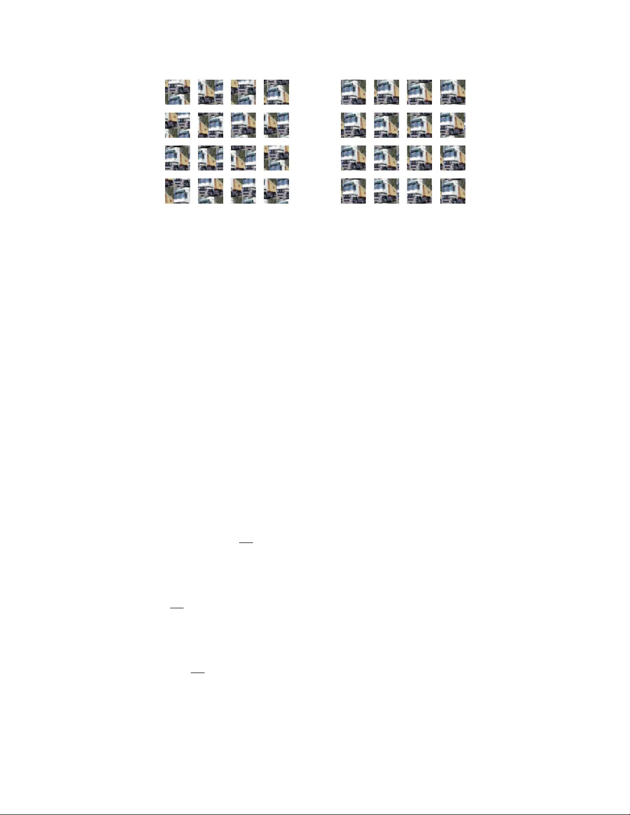
Enhanced Con v olutional Neural T angen t Kernels ∗ Zhiyuan Li † Ruosong W ang ‡ Dingli Y u § Simon S. Du ¶ W ei Hu k Ruslan Salakh utdinov ∗∗ Sanjeev Arora †† Abstract Recen t researc h sho ws that for training with ` 2 loss, conv olutional neural netw orks ( CNN s) whose width (n umber of c hannels in conv olutional la yers) goes to infinity corresp ond to regres- sion with resp ect to the CNN Gaussian Process kernel ( CNN-GP ) if only the last la yer is trained, and corresp ond to regression with resp ect to the Con volutional Neural T angen t Kernel ( CNTK ) if all lay ers are trained. An exact algorithm to compute CNTK [ Arora et al. , 2019 ] yielded the finding that classification accuracy of CNTK on CIF AR-10 is within 6-7% of that of the corre- sp onding CNN architecture (b est figure b eing around 78%) which is interesting p erformance for a fixed kernel. Here we show how to significantly enhance the p erformance of these kernels using tw o ideas. (1) Mo difying the kernel using a new op eration called L o c al A ver age Po oling ( LAP ) whic h pre- serv es efficient computabilit y of the k ernel and inherits the spirit of standard data augmen tation using pixel shifts. Earlier papers were unable to incorporate naiv e data augmen tation because of the quadratic training cost of k ernel regression. This idea is inspired by Glob al Aver age Po oling ( GAP ), which we show for CNN-GP and CNTK is equiv alent to full translation data augmen- tation. (2) Representing the input image using a pre-pro cessing technique prop osed by Coates et al. [ 2011 ], which uses a single conv olutional lay er comp osed of random image patches. On CIF AR-10, the resulting kernel, CNN-GP with LAP and horizontal flip data augmen tation, ac hieves 89% accuracy , matc hing the p erformance of AlexNet [ Krizhevsky et al. , 2012 ]. Note that this is the b est such result we kno w of for a classifier that is not a trained neural net work. Similar impro vemen ts are obtained for F ashion-MNIST. 1 In tro duction Recen t researc h sho ws that for training with ` 2 loss, conv olutional neural netw orks ( CNN s) whose width (num ber of channels in conv olutional lay ers) go es to infinity , corresp ond to regression with resp ect to the CNN Gaussian Pro cess kernel ( CNN-GP ) if only the last lay er is trained, and corre- sp ond to regression with resp ect to the Conv olutional Neural T angent Kernel ( CNTK ) if all lay ers are trained [ Jacot et al. , 2018 ]. An exact algorithm w as giv en [ Arora et al. , 2019 ] to compute ∗ The first three authors contribute equally . † Princeton Universit y . Email: zhiyuanli@cs.princeton.edu . ‡ Carnegie Mellon Universit y . Email: ruosongw@andrew.cmu.edu . § Princeton Universit y . Email: dingliy@cs.princeton.edu . ¶ Institute for Adv anced Study . Email: ssdu@ias.edu . k Princeton Universit y . Email: huwei@cs.princeton.edu . ∗∗ Carnegie Mellon Universit y . Email: rsalakhu@cs.cmu.edu . †† Princeton Universit y and Institute for Adv anced Study . Email: arora@cs.princeton.edu . 1 CNTK for CNN architectures, as w ell as those that include a Glob al Aver age Po oling ( GAP ) la yer (defined b elow). This is a fixed k ernel that inherits some b enefits of CNN s, including exploitation of lo cality via conv olution, as well as m ultiple lay ers of pro cessing. F or CIF AR-10, incorp orating GAP in to the k ernel improv es classification accuracy b y up to 10% compared to pure con volutional CNTK . While this p erformance is encouraging for a fixed k ernel, the b est accuracy is still under 78%, whic h is disapp ointing even compared to AlexNet. One hop e for improving the accuracy further is to somehow capture mo dern innov ations suc h as batc h normalization, data augmentation, residual la yers, etc. in CNTK . The curren t pap er shows ho w to incorp orate simple data augmentation. Sp ecifically , the idea of creating new training images from existing images using pixel translation and flips, while assuming that these op erations should not c hange the lab el. Since deep learning uses sto c hastic gradient descen t (SGD), it is trivial to do suc h data augmen tation on the fly . How ever, it’s unclear ho w to efficien tly incorporate data augmentation in k ernel regression, since training time is quadratic in the n umber of training images. Th us somehow data augmentation has to b e incorp orated into the computation of the kernel itself. The main observ ation here is that the ab ov e-mentioned algorithm for computing CNTK in- v olves a dynamic programming whose recursion depth is equal to the depth of the corresp onding finite CNN . It is p ossible to imp ose symmetry constrain ts at an y desired lay er during this com- putation. In this viewp oint, it can b e shown that prediction using CNTK / CNN-GP with GAP is equiv alent to prediction using CNTK / CNN-GP without GAP but with ful l tr anslation data augmen- tation with wrap-around at the b oundary . The translation inv ariance prop erty implicitly assumed in data augmentation is exactly equiv alen t to an imp osed symmetry constraint in the computation of the CNTK whic h in turn is derived from the p o oling la yer in the CNN . See Section 4 for more details. Th us GAP corresp onds to full translation data augmentation scheme, but in practice suc h data augmen tation creates unrealistic images (cf. Figure 1 ) and training on them can harm p erformance. Ho wev er, the idea of incorp orating symmetry in the dynamic programming leads to a v ariant we call L o c al Aver age Po oling ( LAP ). This implicitly is like data augmen tation where image lab els are assumed to b e inv ariant to small translation, sa y by a few pixels. This op eration also suggests a new p o oling la yer for CNN s which w e call BBlur and also find it b eneficial for CNN s in exp eriments. Exp erimen tally , we find LAP significan tly enhances the p erformance as discussed b elow. • In extensive exp eriments on CIF AR-10 and F ashion-MNIST, w e find that LAP consistently im- pro ves p erformance of CNN-GP and CNTK . In particular, w e find CNN-GP with LAP achiev es 81% on CIF AR-10 dataset, outp erforming the b est previous kernel predictor by 3%. • When using the technique prop osed by Coates et al. [ 2011 ], which uses randomly sampled patc hes from training data as filters to do pre-pro cessing, 1 CNN-GP with LAP and horizon tal flip data augmen tation achiev es 89% accuracy on CIF AR-10, matc hing the p erformance of AlexNet [ Krizhevsky et al. , 2012 ] and is the strongest classifier that is not a trained neural net work. 2 • W e also derive a lay er for CNN that corresp onds to LAP and observe that it improv es the p erformance on certain arc hitectures. 1 See Section 6.2 for the precise pro cedure. 2 h ttps://b enchmarks.ai/cifar-10 2 2 Related W ork Data augmen tation has long b een kno wn to improv e the p erformance of neural netw orks and k ernel metho ds [ Sietsma and Do w , 1991 , Sch¨ olk opf et al. , 1996 ]. Theoretical study of data augmentation dates back to Chap elle et al. [ 2001 ]. Recently , Dao et al. [ 2018 ] prop osed a theoretical framew ork for understanding data augmentation and sho wed data augmen tation with a k ernel classifier can ha ve feature a veraging and v ariance regularization effects. More recen tly , Chen et al. [ 2019 ] quanti- tativ ely shows in certain settings, data augmentation pro v ably impro ves the classifier p erformance. F or more comprehensiv e discussion on data augmentation and its prop erties, w e refer readers to Dao et al. [ 2018 ], Chen et al. [ 2019 ] and references therein. CNN-GP and CNTK corresp ond to infinitely wide CNN with different training strategies (only training the top lay er or training all la yers jointly). The corresp ondence b etw een infinite neural net works and kernel machines w as first noted b y Neal [ 1996 ]. More recen tly , this was extended to deep and conv olutional neural netw orks [ Lee et al. , 2018 , Matthews et al. , 2018 , Nov ak et al. , 2019 , Garriga-Alonso et al. , 2019 ]. These kernels corresp ond to neural net works where only the last lay er is trained. A recen t line of w ork studied ov erparameterized neural net works where all la yers are trained [ Allen-Zhu et al. , 2018 , Du et al. , 2019b , 2018 , Li and Liang , 2018 , Zou et al. , 2018 ]. Their pro ofs imply the gradient k ernel is close to a fixed kernel which only depends the training data and the neural netw ork architecture. These kernels th us corresp ond to neural net works where are all la yers are trained. Jacot et al. [ 2018 ] named this kernel neural tangent kernel ( NTK ). Arora et al. [ 2019 ] formally prov ed p olynomially wide neural net predictor trained by gradient descen t is equiv alent to NTK predictor. Recently , NTK s induced b y v arious neural netw ork arc hitectures are deriv ed and shown to achiev e strong empirical p erformance [ Arora et al. , 2019 , Y ang , 2019 , Du et al. , 2019a ]. Global Av erage Pooling ( GAP ) is first prop osed in Lin et al. [ 2013 ] and is common in mo dern CNN design [ Springenberg et al. , 2014 , He et al. , 2016 , Huang et al. , 2017 ]. Ho wev er, current theoretical understanding on GAP is still rather limited. It has b een conjectured in Lin et al. [ 2013 ] that GAP reduces the num b er of parameters in the last fully-connected lay er and th us a voids o verfitting, and GAP is more robust to spatial translations of the input since it sums out the spatial information. In this work, we study GAP from the CNN-GP and CNTK p ersp ective, and draw an in teresting connection b etw een GAP and data augmen tation. The approac h prop osed in Coates et al. [ 2011 ] is one of the b est-p erforming approaches on CIF AR-10 preceding mo dern CNNs. In this work we combine CNTK with LAP and the approach in Coates et al. [ 2011 ] to achiev e the b est p erformance for classifiers that are not trained neural net works. 3 Preliminaries 3.1 Notation W e use b old-faced letters for vectors, matrices and tensors. F or a v ector a , w e use [ a ] i to denote its i -th entry . F or a matrix A , w e use [ A ] i,j to denote its ( i, j )-th entry . F or an order 4 tensor T , we use [ T ] i,j,i 0 ,j 0 to denote its ( i, j, i 0 , j 0 )-th en try . F or an order 4 tensor, w et use tr ( T ) to denote P i,j T i,j,i,j . F or an order d tensor T ∈ R C 1 × C 2 × ... × C d and an in teger α ∈ [ C d ], w e use T ( α ) ∈ R C 1 × C 2 × ... × C d − 1 to denote the order d − 1 tensor formed by fixing the co ordinate of the last dimension to b e α . 3 3.2 CNN , CNN-GP and CNTK In this section w e giv e formal definitions of CNN , CNN-GP and CNTK that w e study in this pap er. Throughout the pap er, w e let P b e the width and Q b e the heigh t of the image. W e use q ∈ Z + to denote the filter size. In practice, q = 1, 3, 5 or 7. P adding Schemes. In the definition of CNN , CNTK and CNN-GP , we may use differen t padding sc hemes. Let x ∈ R P × Q b e an image. F or a given index pair ( i, j ) with i ≤ 0, i ≥ P + 1, j ≤ 0 or j ≥ Q + 1, differen t padding schemes define differen t v alue for [ x ] i,j . F or cir cular p adding , w e define [ x ] i,j to b e [ x ] i mod P ,j mo d Q . F or zer o p adding , we simply define [ x ] i,j to b e 0. Note the difference b etw een circular padding and zero padding o ccurs only on the b oundary of images. W e will pro ve our theoretical results for the circular padding scheme to av oid b oundary effects. CNN . Now we describ e CNN with and without GAP . F or any input image x , after L in termediate la yers, we obtain x ( L ) ∈ R P × Q × C ( L ) where C ( L ) is the num b er of channels of the last la yer. See Section A for the definition of x ( L ) . F or the output, there are tw o choices: with and without GAP . • Without GAP : the final output is defined as f ( θ , x ) = C ( L ) X α =1 D W ( L +1) ( α ) , x ( L ) ( α ) E where x ( L ) ( α ) ∈ R P × Q , and W ( L +1) ( α ) ∈ R P × Q is the w eight of the last fully-connected lay er. • With GAP : the final output is defined as f ( θ , x ) = 1 P Q C ( L ) X α =1 W ( L +1) ( α ) · X ( i,j ) ∈ [ P ] × [ Q ] h x ( L ) ( α ) i i,j where W ( L +1) ( α ) ∈ R is the w eight of the last fully-connected lay er. CNN-GP and CNTK . No w we describ e CNN-GP and CNTK . Let x , x 0 b e tw o input images. W e denote the L -th lay er’s CNN-GP k ernel as Σ ( L ) ( x , x 0 ) ∈ R [ P ] × [ Q ] × [ P ] × [ Q ] and the L -th lay er’s CNTK kernel as Θ ( L ) ( x , x 0 ) ∈ R [ P ] × [ Q ] × [ P ] × [ Q ] . See Section A for the precise definitions of Σ ( L ) ( x , x 0 ) and Θ ( L ) ( x , x 0 ). F or the output k ernel v alue, again, there are t wo choices, without GAP (equiv alent to using a fully-connected lay er) or with GAP . • Without GAP : the output of CNN-GP is Σ FC  x , x 0  = tr  Σ ( L ) ( x , x 0 )  and the output of CNTK is Θ FC  x , x 0  = tr  Θ ( L ) ( x , x 0 )  . 4 • With GAP : the output of CNN-GP is Σ GAP  x , x 0  = 1 P 2 Q 2 X i,j,i 0 ,j 0 ∈ [ P ] × [ Q ] × [ P ] × [ Q ] h Σ ( L )  x , x 0  i i,j,i 0 ,j 0 and the output of CNTK is Θ GAP  x , x 0  = 1 P 2 Q 2 X i,j,i 0 ,j 0 ∈ [ P ] × [ Q ] × [ P ] × [ Q ] h Θ ( L )  x , x 0  i i,j,i 0 ,j 0 . Kernel Prediction. Lastly , w e recall the formula for kernel regression. F or simplicit y , through- out the pap er, w e will assume all k ernels are in vertible. Giv en a k ernel K ( x , x 0 ) and a dataset ( X , y ) with data { ( x i , y i ) } N i =1 , define K X ∈ R N × N to b e [ K X ] i,j = K ( x i , x j ). The prediction for an unseen data x 0 is P N i =1 α i K ( x 0 , x i ) where α = K − 1 X y . 3.3 Data Augmen tation Sc hemes In this pap er w e consider t wo types of data augmen tation sc hemes: translation and horizon tal flip. T ranslation. Given ( i, j ) ∈ [ P ] × [ Q ], w e define the translation op erator T i,j : R P × Q × C → R P × Q × C as follo w. F or an image x ∈ R P × Q × C , [ T i,j ( x )] i 0 ,j 0 ,c = [ x ] i 0 + i,j 0 + j,c for ( i 0 , j 0 , c ) ∈ [ P ] × [ Q ] × [ C ]. Here the precise definition of [ x ] i 0 + i,j 0 + j,c dep ends on the padding sc heme. Giv en a dataset D = { ( x i , y i ) } N i =1 , the ful l tr anslation data augmentation scheme creates a new dataset D T = { ( T i,j ( x i ) , y i ) } ( i,j,n ) ∈ [ P ] × [ Q ] × [ N ] and training is p erformed on D T . Horizon tal Flip. F or an image x ∈ R P × Q × C , the flip op erator F : R P × Q × C → R P × Q × C is defined to b e [ F ( x )] i,j,c = [ x ] P +1 − i,j,c for ( i, j, c ) ∈ [ P ] × [ Q ] × [ C ]. Giv en a dataset D = { ( x i , y i ) } N i =1 , the horizontal flip data augmentation scheme creates a new dataset of the form D F = { ( F ( x i ) , y i ) } N i =1 and training is p erformed on D F ∪ D . 4 Equiv alence Bet w een Augmen ted Kernel and Data Augmenta- tion In this section, we demonstrate the equiv alence betw een data augmentation and augmen ted k ernels. T o formally discuss the equiv alence, we use group theory to describ e translation and horizontal flip op erators. W e pro vide the definition of group in Section B for completeness. It is easy to v erify that {F , I } , {T i,j } ( i,j ) ∈ [ P ] × [ Q ] , {T i,j ◦ F } ( i,j ) ∈ [ P ] × [ Q ] ∪ {T i,j } ( i,j ) ∈ [ P ] × [ Q ] are groups, where I is the identit y map. F rom now on, giv en a dataset ( X , y ) with data { ( x i , y i ) } N i =1 and a group G , the augmen ted dataset ( X G , y G ) is defined to b e { g ( x i ) , y i } g ∈G ,i ∈ [ N ] . The prediction for an unseen data x 0 on the augmen ted dataset is P i ∈ [ N ] ,g ∈G e α i,g K ( x 0 , g ( x i )) where e α =  K X G  − 1 y G . 5 T o pro ceed, we define the concept of augmente d kernel . Let G b e a finite group. Define the augmen ted kernel K G as K G ( x , x 0 ) = E g ∈G K ( g ( x ) , x 0 ) where x , x 0 are t w o inputs images and g is dra wn from G uniformly at random. A k ey observ ation is that for CNTK and CNN-GP , when circular padding and GAP is adopted, the corresp onding kernel is the augmen ted kernel of the group G = {T i,j } ( i,j ) ∈ [ P ] × [ Q ] . F ormally , w e hav e Σ GAP  x , x 0  = 1 P Q Σ G FC  x , x 0  and Θ GAP  x , x 0  = 1 P Q Θ G FC  x , x 0  , whic h can b e seen by c hecking the form ula of these kernels and using definition of circular padding. Similarly , the follo wing equiv ariance property holds for Σ GAP , Σ FC , Θ GAP and Θ FC , under all groups men tioned ab ov e, including {F , I } and {T i,j } ( i,j ) ∈ [ P ] × [ Q ] . Definition 4.1. A kernel K is equiv ariant under a gr oup G if and only if for any g ∈ G , K ( g ( x ) , g ( x 0 )) = K ( x , x 0 ) . The following theorem formally states the equiv alence b etw een using an augmented kernel on the dataset and using the k ernel on the augmented dataset. Theorem 4.1. Given a gr oup G and a kernel K such that K is e quivariant under G , then the pr e diction of augmente d kernel K G with dataset ( X , y ) is e qual to that of kernel K and augmente d dataset ( X G , y G ) . Namely, for any x 0 ∈ R P × Q × C , P N i =1 α i K G ( x 0 , x i ) = P i ∈ [ N ] ,g ∈G e α i,g K ( x 0 , g ( x i )) wher e α =  K G X  − 1 y , e α =  K X G  − 1 y G . The pro of is deferred to App endix B . Theorem 4.1 implies the follo wing tw o corollaries. Corollary 4.1. F or G = {T i,j } ( i,j ) ∈ [ P ] × [ Q ] , for any given dataset D , the pr e diction of Σ GAP (or Θ GAP ) with dataset D is e qual to the pr e diction of Σ FC (or Θ FC ) with augmente d dataset D T . Corollary 4.2. F or G = {F , I } , for any given dataset D , the pr e diction of Σ G GAP (or Θ G GAP ) with dataset D is e qual to the pr e diction of Σ GAP (or Θ GAP ) with augmente d dataset D F ∪ D . No w w e discuss implications of Theorem 4.1 and its corollaries. Naiv ely applying data augmen- tation, with full translation on CNTK or CNN-GP for example, one needs to create a muc h larger k ernel matrix since there are P Q translation op erators, whic h is often computationally infeasible. Instead, one can directly use the augmen ted k ernel ( Σ GAP or Θ GAP for the case of full translation on CNTK or CNN-GP ) for prediction, for which one only needs to create a k ernel matrix that is as large as the original one. F or horizontal flip, although the augmentation k ernel can not b e conv eniently computed as full translation, Corollary 4.2 still provides a more efficient metho d for computing k ernel v alues and solving k ernel regression, since the augmented dataset is twice as large as the original dataset, while the k ernel matrix of the augmented kernel is as large as the original one. 6 (a) GAP (b) LAP with c = 4 Figure 1: Randomly sampled images with full translation data augmentation and lo cal translation data augmen tation from CIF AR-10. F ull translation data augmentation can create unrealistic im- ages that harm the p erformance whereas lo cal translation data augmen tation creates more realistic images. 5 Lo cal Av erage P o oling In this section, w e in tro duce a new op eration called L o c al Aver age Po oling ( LAP ). As discussed in the in tro duction, full translation data augmen tation ma y create unrealistic images. A natural idea is to do lo cal translation data augmen tation, i.e., restricting the distance of translation. More sp ecifically , w e only allow translation op erations T ∆ i , ∆ j (cf. Section 3.3 ) for (∆ i , ∆ j ) ∈ [ − c, c ] × [ − c, c ] where c is a parameter to control the amoun t of allow ed translation. With a prop er c hoice of the parameter c , translation data augmen tation will not create unrealistic images (cf. Figure 1 ). How ever, naiv e lo cal translation data augmentation is computationally infeasible for kernel metho ds, even for mo derate choice of c . T o remedy this issue, in this section we introduce LAP , whic h is inspired b y the connection b et ween full translation data augmentation and GAP on CNN-GP and CNTK . Here, for simplicity , we assume P = Q and deriv e the form ula only for CNTK . Our form ula can b e generalized to CNN-GP in a straigh tforward manner. Recall that for tw o giv en images x and x 0 , without GAP , the form ula for output of CNTK is tr ( Θ ( x , x 0 )). With GAP , the formula for output of CNTK is 1 P 4 X i,j,i 0 ,j 0 ∈ [ P ] 4  Θ  x , x 0  i,j,i 0 ,j 0 . With circular padding, the form ula can b e rewritten as 1 P 2 E ∆ i , ∆ 0 i , ∆ j , ∆ 0 j ∼ [ P ] 4 X i,j ∈ [ P ] × [ P ]  Θ  x , x 0  i +∆ i ,j +∆ j ,i +∆ 0 i ,j +∆ 0 j , whic h is again equal to 1 P 2 E ∆ i , ∆ 0 i , ∆ j , ∆ 0 j ∼ [ P ] 4 tr  Θ  T ∆ i , ∆ j ( x ) , T ∆ 0 i , ∆ 0 j ( x 0 )  . W e ignore the 1 /P 2 scaling factor since it pla ys no role in kernel regression. 7 No w we consider restricted translation op erations T ∆ i , ∆ j with (∆ i , ∆ j ) ∈ [ − c, c ] × [ − c, c ] and deriv e the formula for LAP . Assuming circular padding, we hav e E ∆ i , ∆ 0 i , ∆ j , ∆ 0 j ∼ [ − c,c ] 4 tr  Θ  T ∆ i , ∆ j ( x ) , T ∆ 0 i , ∆ 0 j ( x 0 )  = 1 (2 c + 1) 4 X ∆ i , ∆ 0 i , ∆ j , ∆ 0 j ∈ [ − c,c ] 4 X i,j ∈ [ P ] 2  Θ ( x , x 0 )  i +∆ i ,j +∆ j ,i +∆ 0 i ,j +∆ 0 j . (1) No w we ha ve derived the form ula for LAP , which is the RHS of Equation 1 . Notice that the form ula in the RHS of Equation 1 is a w ell-defined quantit y for all padding sc hemes. In particular, assuming zero padding, when c = P , LAP is equiv alent to GAP . When c = 0, LAP is equiv alent to no p o oling lay er. Another adv antage of LAP is that it do es not incur any extra computational cost, since the form ula in Equation 1 can b e rewritten as X i,j,i 0 ,j 0 ∈ [ P ] 4 [ w ] i,j,i 0 ,j 0 ·  Θ ( x , x 0 )  i,j,i 0 ,j 0 where eac h entry in the weigh t tensor w can b e calculated in constant time. Note that the GAP op eration in CNN-GP and CNTK corresp onds to the GAP la yer in CNN s. Here we observe that the follo wing b ox blur layer corresp onds to LAP in CNN s. Bo x blur lay er ( BBlur ) is a function R P × Q → R P × Q suc h that [ BBlur ( x )] i,j = 1 (2 c + 1) 2 X ∆ i , ∆ j ∈ [ − c,c ] 2 x i +∆ i ,j +∆ j . This is in fact the standard a verage p o oling lay er with p o oling size 2 c + 1 and stride 1. W e prov e the equiv alence b etw een LAP and b o x blur lay er in App endix C . In Section 6.3 , we v erify the effectiv eness of BBlur on CNN s via exp eriments. 6 Exp erimen ts In this section we present our empirical findings on CIF AR-10 [ Krizhevsky , 2009 ] and F ashion- MNIST [ Xiao et al. , 2017 ]. Exp erimen tal Setup. F or b oth CIF AR-10 and F ashion-MNIST we use the full training set and rep ort the test accuracy on the full test set. Throughout this section we only consider 3 × 3 con volutional filters with stride 1 and no dilation. In the con volutional la yers in CNTK and CNN- GP , we use zero padding with pad size 1 to ensure the input of eac h la yer has the same size. W e use zero padding for LAP throughout the exp eriment. W e p erform standard prepro cessing (mean subtraction and standard deviation division) for all images. In all exp eriments, we p erform kernel ridge regression to utilize the calculated kernel v alues 3 . W e normalize the kernel matrices so that all diagonal en tries are ones. Equiv alen tly , w e ensure all features hav e unit norm in RKHS. Since the resulting kernel matrices are usually ill-conditioned, w e set the regularization term λ = 5 × 10 − 5 , to make inv erting k ernel matrices n umerically stable. 3 W e also tried kernel SVM but found it significantly degrading the p erformance, and thus do not include the results. 8 c d 5 8 11 14 0 66 . 55 (69 . 87) 66 . 27 (69 . 87) 65 . 85 (69 . 37) 65 . 47 (68 . 90) 4 77 . 06 (79 . 08) 77 . 14 (78 . 96) 77 . 06 (78 . 98) 76 . 52 (78 . 74) 8 79 . 24 (80 . 95) 79 . 25 (81 . 03) 78 . 98 (80 . 94) 78 . 65 (80 . 35) 12 80 . 11 (81 . 34) 79 . 79 (81 . 28) 79 . 29 (81 . 14) 79 . 13 (80 . 91) 16 79 . 80 (81 . 21) 79 . 71 ( 81 . 40 ) 79 . 74 (81 . 09) 79 . 42 (81 . 00) 20 79 . 24 (80 . 67) 79 . 27 (80 . 88) 79 . 30 (80 . 76) 78 . 92 (80 . 39) 24 78 . 07 (79 . 88) 78 . 16 (79 . 79) 78 . 14 (80 . 06) 77 . 87 (80 . 07) 28 76 . 91 (78 . 69) 77 . 33 (79 . 20) 77 . 65 (79 . 56) 77 . 65 (79 . 74) 32 76 . 79 (78 . 53) 77 . 39 (79 . 13) 77 . 63 (79 . 51) 77 . 63 (79 . 74) T able 1: T est accuracy of CNTK on CIF AR-10. W e use one-hot enco dings of the lab els as regression targets. W e use scipy.linalg.solve to solv e the corresp onding k ernel ridge regression problem. The k ernel v alue of CNTK and CNN-GP are calculated using the CuPy pack age. W e write nativ e CUD A co des to sp eed up the calculation of the kernel v alues. All exp eriments are p erformed on Amazon W eb Services (A WS), using (p ossibly m ultiple) NVIDIA T esla V100 GPUs. F or efficiency considerations, all k ernel v alues are computed with 32-bit precision. One unique adv antage of the dynamic programming algorithm for calculating CNTK and CNN- GP is that we do not need rep eat exp eriments for, say , differen t v alues of c in LAP and different depths. With our highly-optimized native CUD A co des, w e sp end roughly 1,000 GPU hours on calculating all k ernel v alues for eac h dataset. 6.1 Ablation Study on CIF AR-10 and F ashion-MNIST W e p erform exp erimen ts to study the effect of different v alues of the c parameter in LAP and horizon tal flip data argumen tation on CNTK and CNN-GP . F or exp eriments in this section we set the bias term in CNTK and CNN-GP to b e γ = 0 (cf. Section A ). W e use the same architecture for CNTK and CNN-GP as in Arora et al. [ 2019 ]. I.e., w e stack multiple con volutional lay ers b efore the final p o oling lay er. W e use d to denote the n umber of con volutions lay ers, and in our exp erimen ts w e set d to b e 5, 8, 11 or 14, to study the effect of depth on CNTK and CNN-GP . F or CIF AR-10, w e set the c parameter in LAP to b e 0 , 4 , . . . , 32, while for F ashion-MNIST we set the c parameter in LAP to b e 0 , 4 , . . . , 28. Notice that when c = 32 for CIF AR-10 or c = 28 for F ashion-MNIST, LAP is equiv alent to GAP , and when c = 0, LAP is equiv alen t to no p o oling la yer. Results on CIF AR-10 are rep orted in T ables 1 and 2 , and results on F ashion-MNIST are rep orted in T ables 3 and 4 . In each table, for each com bination of c and d , the first num b er is the test accuracy without horizon tal flip data augmentation (in p ercen tage), and the second num b er (in parentheses) is the test accuracy with horizon tal flip data augmentation. 9 c d 5 8 11 14 0 63 . 53 (67 . 90) 65 . 54 (69 . 43) 66 . 42 (70 . 30) 66 . 81 (70 . 48) 4 76 . 35 (78 . 79) 77 . 03 (79 . 30) 77 . 39 (79 . 52) 77 . 35 (79 . 65) 8 79 . 48 (81 . 32) 79 . 82 (81 . 49) 79 . 76 (81 . 71) 79 . 69 (81 . 53) 12 80 . 40 (82 . 13) 80 . 64 (82 . 09) 80 . 58 (82 . 06) 80 . 32 (81 . 95) 16 80 . 36 (81 . 73) 80 . 78 ( 82 . 20 ) 80 . 59 (82 . 06) 80 . 41 (81 . 83) 20 79 . 87 (81 . 50) 80 . 15 (81 . 33) 79 . 87 (81 . 46) 79 . 98 (81 . 35) 24 78 . 60 (79 . 98) 78 . 91 (80 . 48) 79 . 22 (80 . 53) 78 . 94 (80 . 46) 28 77 . 18 (78 . 84) 78 . 03 (79 . 86) 78 . 45 (79 . 87) 78 . 48 (80 . 07) 32 77 . 00 (78 . 49) 77 . 85 (79 . 65) 78 . 49 (80 . 04) 78 . 45 (80 . 01) T able 2: T est accuracy of CNN-GP on CIF AR-10. c d 5 8 11 14 0 92 . 25 (92 . 56) 92 . 22 (92 . 51) 92 . 11 (92 . 29) 91 . 76 (92 . 17) 4 93 . 76 ( 94 . 07 ) 93 . 69 (93 . 86) 93 . 55 (93 . 74) 93 . 37 (93 . 58) 8 93 . 72 (93 . 96) 93 . 67 (93 . 78) 93 . 50 (93 . 58) 93 . 32 (93 . 51) 12 93 . 59 (93 . 80) 93 . 58 (93 . 70) 93 . 35 (93 . 44) 93 . 21 (93 . 40) 16 93 . 50 (93 . 62) 93 . 42 (93 . 63) 93 . 27 (93 . 40) 93 . 10 (93 . 25) 20 93 . 10 (93 . 34) 93 . 17 (93 . 49) 93 . 20 (93 . 34) 92 . 99 (93 . 18) 24 92 . 77 (93 . 04) 93 . 07 (93 . 44) 93 . 11 (93 . 31) 93 . 02 (93 . 21) 28 92 . 80 (92 . 98) 93 . 08 (93 . 42) 93 . 12 (93 . 28) 92 . 97 (93 . 19) T able 3: T est accuracy of CNTK on F ashion-MNIST. c d 5 8 11 14 0 91 . 47 (91 . 81) 91 . 96 (92 . 37) 92 . 09 (92 . 60) 92 . 22 (92 . 72) 4 93 . 44 (93 . 60) 93 . 59 ( 93 . 79 ) 93 . 63 (93 . 76) 93 . 59 (93 . 64) 8 93 . 26 (93 . 16) 93 . 41 (93 . 51) 93 . 31 (93 . 52) 93 . 39 (93 . 46) 12 92 . 83 (92 . 94) 93 . 07 (93 . 20) 93 . 11 (93 . 15) 92 . 94 (93 . 09) 16 92 . 46 (92 . 51) 92 . 58 (92 . 83) 92 . 64 (92 . 92) 92 . 68 (93 . 07) 20 91 . 83 (91 . 72) 92 . 35 (92 . 42) 92 . 49 (92 . 79) 92 . 51 (92 . 69) 24 91 . 15 (91 . 40) 92 . 10 (92 . 18) 92 . 29 (92 . 60) 92 . 41 (92 . 77) 28 91 . 30 (91 . 37) 92 . 03 (92 . 27) 92 . 41 (92 . 79) 92 . 41 (92 . 74) T able 4: T est accuracy of CNN-GP on F ashion-MNIST. W e made the following observ ations regarding our exp erimental results. • LAP with a prop er c hoice of the parameter c significantly improv es the p erformance of CNTK and CNN-GP . On CIF AR-10, the b est-p erforming v alue of c is c = 12 or 16, while on F ashion-MNIST the b est-p erforming v alue of c is c = 4. W e susp ect this difference is due 10 to the nature of the tw o datasets: CIF AR-10 contains real-life images and th us allow more translation, while F ashion-MNIST contains images with centered clothes and thus allow less translation. F or b oth datasets, the b est-performing v alue of c is consisten t across all settings (depth, CNTK or CNN-GP ) that w e hav e considered. • Horizon tal flip data augmentation is less effectiv e on F ashion-MNIST than on CIF AR-10. There are t wo p ossible explanations for this phenomenon. First, most images in F ashion- MNIST are nearly horizon tally symmetric (e.g., T-shirts and bags). Second, CNTK and CNN-GP hav e already achiev ed a relativ ely high accuracy on F ashion-MNIST, and thus it is reasonable for horizon tal flip data augmentation to b e less effective on this dataset. • Finally , for CNTK , when c = 0 (no p o oling la yer) and c = 32 ( GAP ) our rep orted test accuracies are close to those in Arora et al. [ 2019 ] on CIF AR-10. F or CNN-GP , when c = 0 (no p o oling la yer) our rep orted test accuracies are close to those in No v ak et al. [ 2019 ] on CIF AR-10 and F ashion-MNIST. This suggests that w e hav e repro duced previous rep orted results. 6.2 Impro ving P erformance on CIF AR-10 via Additional Pre-pro cessing Finally , w e explore another interesting question: what is the limit of non-deep-neural-netw ork metho ds on CIF AR-10? T o further improv e the p erformance, we com bine CNTK and CNN-GP with LAP , together with the previous b est-p erforming non-deep-neural-net work metho d Coates et al. [ 2011 ]. Here we use the v ariant implemen ted in Rech t et al. [ 2019 ] 4 . More sp ecifically , w e first sample 2048 random image patches with size 5 × 5 from all training images. Then for the sampled images patches, we subtract the mean of the patches, then normalize them to hav e unit norm, and finally p erform ZCA transformation to the resulting patc hes. W e use the resulting patches as 2048 filters of a conv olutional la yer with kernel size 5, stride 1 and no dilation or padding. F or an input image x , we use conv ( x ) to denote the output of the conv olutional lay er. As in the implementation in Rech t et al. [ 2019 ], we use ReLU( conv ( x ) − γ feature ) and ReLU( − conv ( x ) − γ feature ) as the input feature for CNTK and CNN-GP . Here w e fix γ feature = 1 as in Rec ht et al. [ 2019 ], and set the bias term γ in CNTK and CNN-GP to b e γ = 3, whic h is the filter size used in CNTK and CNN-GP . T o mak e the equiv arian t under horizontal flip (cf. Defin tion 4.1 ), for each image patc h, w e horizontally flip it and add the flipp ed patch in to the conv olutional lay er as a new filter. Th us, for an input CIF AR-10 image of size 32 × 32, the dimension of the output feature is 8192 × 28 × 28. T o isolate the effect of randomness in the choices of the image patc hes, we fix the random seed to be 0 throughout the exp erimen t. In this experiment, we set the v alue of the c parameter in LAP to b e 4 , 8 , 12 , . . . , 20 to av oid small and large v alues of c . The results are rep orted in T ables 5 and 6 . In eac h table, for each combination of c and d , the first num b er is the test accuracy without horizontal flip data augmen tation (in p ercen tage), and the second n umber (in paren theses) is the test accuracy with horizon tal flip data augmentation (again in p ercentage). F rom our exp erimental results, it is evident that combining CNTK or CNN-GP with additional pre-pro cessing can significantly impro ve up on the p erformance of using solely CNTK or CNN-GP , and that of using solely the approac h in Coates et al. [ 2011 ]. Previously , it has been rep orted in Rech t et al. [ 2019 ] that using solely the approach in Coates et al. [ 2011 ] (together with appro- priate p o oling la yer) can only achiev e a test accuracy of 84.2% using 256, 000 image patches, or 4 https://github.com/modestyachts/nondeep 11 c d 5 8 11 14 4 84 . 63 (86 . 64) 84 . 07 (86 . 23) 83 . 29 (85 . 53) 82 . 57 (84 . 81) 8 86 . 36 (88 . 32) 85 . 80 (87 . 81) 85 . 01 (87 . 08) 84 . 57 (86 . 53) 12 86 . 74 (88 . 35) 86 . 20 (87 . 90) 85 . 60 (87 . 36) 84 . 95 (86 . 99) 16 86 . 77 ( 88 . 36 ) 86 . 17 (87 . 85) 85 . 60 (87 . 44) 84 . 92 (86 . 98) 20 86 . 17 (87 . 77) 85 . 71 (87 . 50) 85 . 14 (87 . 07) 84 . 59 (86 . 84) T able 5: T est accuracy of additional pre-pro cessing + CNTK on CIF AR-10. c d 5 8 11 14 4 85 . 49 (87 . 32) 85 . 37 (87 . 22) 85 . 16 (87 . 11) 84 . 79 (86 . 81) 8 87 . 07 (88 . 64) 86 . 82 (88 . 68) 86 . 53 (88 . 40) 86 . 39 (88 . 15) 12 87 . 23 (88 . 91) 87 . 12 ( 88 . 92 ) 86 . 87 (88 . 66) 86 . 62 (88 . 29) 16 87 . 28 (88 . 90) 87 . 11 (88 . 66) 86 . 92 (88 . 61) 86 . 74 (88 . 24) 20 86 . 81 (88 . 26) 86 . 77 (88 . 24) 86 . 61 (88 . 14) 86 . 26 (87 . 84) T able 6: T est accuracy of additional pre-pro cessing + CNN-GP on CIF AR-10. 83.3% using 32, 000 image patches. Even with the help of horizontal flip data augmentation, the approac h in Coates et al. [ 2011 ] can only ac hieve a test accuracy of 85.6% using 256, 000 image patc hes, or 85.0% using 32, 000 image patches. Here we use significan tly less image patches (only 2048 ) but achiev e a m uch b etter p erformance, with the help of CNTK and CNN-GP . In particular, w e achiev e a p erformance of 88.92% on CIF AR-10, matc hing the p erformance of AlexNet on the same dataset. In the setting rep orted in Coates et al. [ 2011 ], increasing the num b er of sampled image patches will further improv e the p erformance. Here w e also conjecture that in our setting, further increasing the n umber of sampled image patches can impro ve the performance and get close to mo dern CNN s. How ev er, due the limitation on computational resources, we lea ve exploring the effect of n umber of sampled image patches as a future research direction. 6.3 Exp erimen ts on CNN with BBlur In Figure 2 , we v erify the effectiveness of BBlur on a 10-la y er CNN (with Batc h Normalization) on CIF AR-10. The setting of this exp eriment is rep orted in App endix D . Our netw ork structure has no p o oling lay er except for the BBlur la yer b efore the final fully-connected lay er. The fully- connected la yer is fixed during the training. Our exp eriment illustrates that even with a fixed final F C lay er, using GAP could improv e the p erformance of CNN , and challenges the conjecture that GAP reduces the num b er of parameters in the last fully-connected lay er and thus a voids o v erfitting. Our exp eriments also show that BBlur with appropriate choice of c achiev es better p erformance than GAP . 12 0 5 10 15 91 92 93 c Accuracy av erage test accuracy best test accuracy (a) With Horizontal Flip Data Augmentation 0 5 10 15 90 91 92 c Accuracy av erage test accuracy best test accuracy (b) Without Horizontal Flip Data Augmentation Figure 2: T est accuracy of 10-la yer CNN with v arious v alues for the c parameter in BBlur . 7 Conclusion In this pap er, inspired by the connection b etw een full translation data augmentation and GAP , we deriv e a new op eration, LAP , on CNTK and CNN-GP , which consisten tly improv es the p erformance on image classification tasks. Com bining CNN-GP with LAP and the pre-pro cessing technique prop osed by Coates et al. [ 2011 ], the resulting kernel achiev es 89% accuracy on CIF AR-10, matc hing the p erformance of AlexNet and is the strongest classifier that is not a trained neural net work. Here we list a few future researc h directions. Is that p ossible to combine more mo dern techniques on CNN , such as batch normalization and residual lay ers, with CNTK or CNN-GP , to further improv e the p erformance? Moreo ver, it is an interesting direction to study other comp onents in mo dern CNN s through the lens of CNTK and CNN-GP . Ac kno wledgemen ts S. Arora, W. Hu, Z. Li and D. Y u are supp orted b y NSF, ONR, Simons F oundation, Schmidt F oundation, Amazon Research, DARP A and SRC. S. S. Du is supp orted b y National Science F oundation (Gran t No. DMS-1638352) and the Infosys Mem b ership. R. Salakh utdinov and R. W ang are supp orted in part by NSF I IS-1763562, Office of Na v al Research grant N000141812861, and Nvidia NV AIL aw ard. P art of this work w as done while R. W ang was visiting Princeton Univ ersity . The authors would lik e to thank Amazon W eb Services for providing compute time for the exp erimen ts in this pap er. References Zeyuan Allen-Zhu, Y uanzhi Li, and Zhao Song. A conv ergence theory for deep learning via ov er- parameterization. arXiv pr eprint arXiv:1811.03962 , 2018. Sanjeev Arora, Simon S Du, W ei Hu, Zhiyuan Li, Ruslan Salakh utdinov, and Ruosong W ang. On exact computation with an infinitely wide neural net. arXiv pr eprint arXiv:1904.11955 , 2019. Olivier Chap elle, Jason W eston, L´ eon Bottou, and Vladimir V apnik. Vicinal risk minimization. In A dvanc es in neur al information pr o c essing systems , pages 416–422, 2001. 13 Sh uxiao Chen, Edgar Dobriban, and Jane H Lee. Inv ariance reduces v ariance: Understanding data augmen tation in deep learning and b eyond. arXiv pr eprint arXiv:1907.10905 , 2019. Adam Coates, Andrew Ng, and Honglak Lee. An analysis of single-la yer netw orks in unsup ervised feature learning. In Pr o c e e dings of the fourte enth international c onfer enc e on artificial intel ligenc e and statistics , pages 215–223, 2011. T ri Dao, Alb ert Gu, Alexander J Ratner, Virginia Smith, Christopher De Sa, and Christopher R´ e. A k ernel theory of mo dern data augmentation. arXiv pr eprint arXiv:1803.06084 , 2018. Simon S Du, Jason D Lee, Hao c huan Li, Liwei W ang, and Xiyu Zhai. Gradient descen t finds global minima of deep neural net works. arXiv pr eprint arXiv:1811.03804 , 2018. Simon S. Du, Kangcheng Hou, Barnab´ as P´ oczos, Ruslan Salakhutdino v, Ruosong W ang, and Keyulu Xu. Graph neural tangent kernel: F using graph neural netw orks with graph k ernels. A rXiv , abs/1905.13192, 2019a. Simon S. Du, Xiyu Zhai, Barnabas Poczos, and Aarti Singh. Gradien t descent prov ably optimizes o ver-parameterized neural netw orks. In International Confer enc e on L e arning R epr esentations , 2019b. Adri Garriga-Alonso, Carl Edward Rasmussen, and Laurence Aitc hison. Deep conv olutional net- w orks as shallow gaussian pro cesses. In International Confer enc e on L e arning R epr esentations , 2019. URL https://openreview.net/forum?id=Bklfsi0cKm . Kaiming He, Xiangyu Zhang, Shao qing Ren, and Jian Sun. Deep residual learning for image recognition. In Pr o c e e dings of the IEEE c onfer enc e on c omputer vision and p attern r e c o gnition , pages 770–778, 2016. Gao Huang, Zhuang Liu, Laurens V an Der Maaten, and Kilian Q W einberger. Densely connected con volutional netw orks. In Pr o c e e dings of the IEEE c onfer enc e on c omputer vision and p attern r e c o gnition , pages 4700–4708, 2017. Arth ur Jacot, F ranck Gabriel, and Cl´ ement Hongler. Neural tangent k ernel: Conv ergence and generalization in neural net works. arXiv pr eprint arXiv:1806.07572 , 2018. Alex Krizhevsky . Learning m ultiple lay ers of features from tiny images. 2009. Alex Krizhevsky , Ilya Sutsk ever, and Geoffrey E Hin ton. Imagenet classification with deep con v olu- tional neural net works. In A dvanc es in neur al information pr o c essing systems , pages 1097–1105, 2012. Jaeho on Lee, Jascha Sohl-dickstein, Jeffrey Pennington, Roman No v ak, Sam Schoenholz, and Y asaman Bahri. Deep neural netw orks as gaussian pro cesses. In International Confer enc e on L e arning R epr esentations , 2018. URL https://openreview.net/forum?id=B1EA- M- 0Z . Y uanzhi Li and Yingyu Liang. Learning ov erparameterized neural net works via sto c hastic gradient descen t on structured data. arXiv pr eprint arXiv:1808.01204 , 2018. Min Lin, Qiang Chen, and Shuic heng Y an. Netw ork in netw ork. arXiv pr eprint arXiv:1312.4400 , 2013. 14 Alexander G de G Matthews, Mark Ro wland, Jiri Hron, Richard E T urner, and Zoubin Ghahramani. Gaussian pro cess b ehaviour in wide deep neural net works. arXiv pr eprint arXiv:1804.11271 , 2018. Radford M Neal. Priors for infinite netw orks. In Bayesian L e arning for Neur al Networks , pages 29–53. Springer, 1996. Roman Nov ak, Lechao Xiao, Y asaman Bahri, Jaeho on Lee, Greg Y ang, Daniel A. Ab olafia, Jef- frey Pennington, and Jascha Sohl-dickstein. Bay esian deep conv olutional netw orks with many c hannels are gaussian pro cesses. In International Confer enc e on L e arning R epr esentations , 2019. URL https://openreview.net/forum?id=B1g30j0qF7 . Benjamin Rech t, Reb ecca Ro elofs, Ludwig Schmidt, and V aishaal Shank ar. Do imagenet classifiers generalize to imagenet? arXiv pr eprint arXiv:1902.10811 , 2019. Bernhard Sc h¨ olkopf, Chris Burges, and Vladimir V apnik. Incorp orating in v ariances in supp ort v ector learning machines. In International Confer enc e on Artificial Neur al Networks , pages 47– 52. Springer, 1996. Jo celyn Sietsma and Rob ert JF Dow. Creating artificial neural net works that generalize. Neur al networks , 4(1):67–79, 1991. Jost T obias Springenberg, Alexey Dosovitskiy , Thomas Bro x, and Martin Riedmiller. Striving for simplicit y: The all con volutional net. arXiv pr eprint arXiv:1412.6806 , 2014. Han Xiao, Kashif Rasul, and Roland V ollgraf. F ashion-mnist: a no vel image dataset for b ench- marking mac hine learning algorithms, 2017. Greg Y ang. Scaling limits of wide neural netw orks with weigh t sharing: Gaussian process b ehavior, gradien t indep endence, and neural tangent kernel deriv ation. arXiv pr eprint arXiv:1902.04760 , 2019. Difan Zou, Y uan Cao, Dongruo Zhou, and Quanquan Gu. Sto chastic gradient descent optimizes o ver-parameterized deep ReLU netw orks. arXiv pr eprint arXiv:1811.08888 , 2018. 15 A F ormal Definitions of CNN , CNN-GP and CNTK In this section we use the following additional notations. Let I be the iden tity matrix, and [ n ] = { 1 , 2 , . . . , n } . Let e i b e an indicator vector with i -th en try b eing 1 and other entries b eing 0, and let 1 denote the all-one vector. W e use  to denote the p oint wise pro duct and ⊗ to denote the tensor pro duct. W e use diag( · ) to transform a vector to a diagonal matrix. W e use σ ( · ) to denote the activ ation function, such as the rectified linear unit (ReLU) function: σ ( z ) = max { z , 0 } , and ˙ σ ( · ) to denote the deriv ative of σ ( · ). Moreo ver, c σ is a fixed constan t. Denote by N ( µ , Σ ) the Gaussian distribution with mean µ and co v ariance Σ . W e first define the con volution op eration. F or a con volutional filter w ∈ R q × q and an image x ∈ R P × Q , the con volution op erator is defined as [ w ∗ x ] i,j = q − 1 2 X a = − q − 1 2 q − 1 2 X b = − q − 1 2 [ w ] a + q +1 2 ,b + q +1 2 [ x ] a + i,b + j for i ∈ [ P ] , j ∈ [ Q ] . (2) Here the precise definition of [ w ] a + q +1 2 ,b + q +1 2 and [ x ] a + i,b + j dep ends on the padding scheme (cf. Section 3.2 ). Notice that in Equation 2 , the v alue of [ w ∗ x ] i,j dep ends on [ x ] i − q − 1 2 : i + q − 1 2 ,j − q − 1 2 : j + q − 1 2 . Th us, for ( i, j, i 0 , j 0 ) ∈ [ P ] × [ Q ] × [ P ] × [ Q ], we define D ij,i 0 j 0 =  ( i + a, j + b, i 0 + a 0 , j 0 + b 0 ) ∈ [ P ] × [ Q ] × [ P ] × [ Q ] | − ( q − 1) / 2 ≤ a, b, a 0 , b 0 ≤ ( q − 1) / 2  . No w we formally define CNN , CNN-GP and CNTK . CNN . • Let x (0) = x ∈ R P × Q × C (0) b e the input image where C (0) is the initial n umber of channels. • F or h = 1 , . . . , L , β = 1 , . . . , C ( h ) , the in termediate outputs are defined as ˜ x ( h ) ( β ) = C ( h − 1) X α =1 W ( h ) ( α ) , ( β ) ∗ x ( h − 1) ( α ) + γ · b ( β ) , x ( h ) ( β ) = r c σ C ( h ) × q × q σ  ˜ x ( h ) ( β )  where each W ( h ) ( α ) , ( β ) ∈ R q × q is a filter with Gaussian initialization, b ( β ) is a bias term with Gaussian initialization, and γ is the scaling factor for the bias term. CNN-GP and CNTK . • F or α = 1 , . . . , C (0) , ( i, j, i 0 , j 0 ) ∈ [ P ] × [ Q ] × [ P ] × [ Q ], define K (0) ( α )  x , x 0  = x ( α ) ⊗ x 0 ( α ) and h Σ (0) ( x , x 0 ) i ij,i 0 j 0 = C (0) X α =1 tr  h K (0) ( α ) ( x , x 0 ) i D ij,i 0 j 0  + γ 2 . • F or h ∈ [ L − 1], 16 – F or ( i, j, i 0 , j 0 ) ∈ [ P ] × [ Q ] × [ P ] × [ Q ], define Λ ( h ) ij,i 0 j 0 ( x , x 0 ) =  Σ ( h − 1) ( x , x )  ij,ij  Σ ( h − 1) ( x , x 0 )  ij,i 0 j 0  Σ ( h − 1) ( x 0 , x )  i 0 j 0 ,ij  Σ ( h − 1) ( x 0 , x 0 )  i 0 j 0 ,i 0 j 0 ! ∈ R 2 × 2 . – F or ( i, j, i 0 , j 0 ) ∈ [ P ] × [ Q ] × [ P ] × [ Q ], define h K ( h ) ( x , x 0 ) i ij,i 0 j 0 = c σ q 2 · E ( u,v ) ∼N  0 , Λ ( h ) ij,i 0 j 0 ( x , x 0 )  [ σ ( u ) σ ( v )] , (3) h ˙ K ( h ) ( x , x 0 ) i ij,i 0 j 0 = c σ q 2 · E ( u,v ) ∼N  0 , Λ ( h ) ij,i 0 j 0 ( x , x 0 )  [ ˙ σ ( u ) ˙ σ ( v )] . (4) – F or ( i, j, i 0 , j 0 ) ∈ [ P ] × [ Q ] × [ P ] × [ Q ], define h Σ ( h ) ( x , x 0 ) i ij,i 0 j 0 =tr  h K ( h ) ( x , x 0 ) i D ij,i 0 j 0  + γ 2 . Note that the definition of Σ ( x , x 0 ) and ˙ Σ ( x , x 0 ) share similar patterns as their NTK coun ter- parts [ Jacot et al. , 2018 ]. The only difference is that we hav e one more step, taking the trace o ver patc hes. This step represents the conv olution op eration in the corresp onding CNN . No w w e can define the k ernel v alue recursiv ely . 1. First, w e define Θ (0) ( x , x 0 ) = Σ (0) ( x , x 0 ). 2. F or h ∈ [ L − 1] and ( i, j, i 0 , j 0 ) ∈ [ P ] × [ Q ] × [ P ] × [ Q ], we define h Θ ( h ) ( x , x 0 ) i ij,i 0 j 0 = tr  h ˙ K ( h ) ( x , x 0 )  Θ ( h − 1) ( x , x 0 ) + K ( h ) ( x , x 0 ) i D ij,i 0 j 0  + γ 2 . 3. Finally , define Θ ( L ) ( x , x 0 ) = ˙ K ( L ) ( x , x 0 )  Θ ( L − 1) ( x , x 0 ) + K ( L ) ( x , x 0 ) . B Additional Definitions and Pro of of Theorem 4.1 Definition B.1 (Group of Op erators) . ( G , ◦ ) is a group of op er ators, if and only if 1. Each element g ∈ G is an op er ator: R P × Q × C → R P × Q × C ; 2. ∀ g 1 , g 2 ∈ G , g 1 ◦ g 2 ∈ G , wher e ( g 1 ◦ g 2 )( x ) is define d as g 1 ( g 2 ( x )) . 3. ∃ e ∈ G , such that ∀ g ∈ G , e ◦ g = g ◦ e = g . 4. ∀ g 1 ∈ G , ∃ g 2 ∈ G , such that g 1 ◦ g 2 = g 2 ◦ g 1 = e . We say g 2 is the inverse of g 1 , namely, g 2 = g − 1 1 . 17 Pr o of of The or em 4.1 . Since we assume K G X and K X G are inv ertible, b oth α and e α are uniquely defined. No w w e claim e α g = { e α i,g } i ∈ [ N ] ∈ R N is equal to α |G | for all g ∈ G . By the equiv ariance of K under G , for all j ∈ [ N ] and g 0 ∈ G , X i ∈ [ N ] ,g ∈G α i |G | K ( g 0 ( x j ) , g ( x i )) = X i ∈ [ N ] ,g ∈G α i |G | K (( g − 1 ◦ g 0 )( x j ) , x i ) = X i ∈ [ N ] α i E g ∈G K ( g ( x j ) , x i ) = X i ∈ [ N ] α i K G ( x j , x i ) = y j . Note that e α is defined as the unique solution of K X G e α = y G . Similarly , we hav e X i ∈ [ N ] ,g ∈G α i |G | K ( x 0 , g ( x i )) = X i ∈ [ N ] α i E g ∈G K ( g − 1 ( x 0 ) , x i ) = X i ∈ [ N ] α i K G ( x 0 , x i ) . C Equiv alence Bet w een LAP and Bo x Blur La y er. F or a CNN with a b o x blur lay er b efore the final fully-connected lay er, the final output is defined as f ( θ , x ) = P C ( L ) α =1 D W ( L +1) ( α ) , BBlur  x ( L ) ( α ) E , where x ( L ) ( α ) ∈ R P × Q , and W ( L +1) ( α ) ∈ R P × Q is the weigh t of the last fully-connected la yer. No w we establish the equiv alence b etw een BBlur and LAP on CNTK . The equiv alence on CNN-GP can b e derived similarly . Let Θ BBlur ( x , x 0 ) ∈ R [ P ] × [ Q ] × [ P ] × [ Q ] b e the CNTK kernel of BBlur  x ( L ) ( α )  . Since BBlur is just a linear op eration, we hav e  Θ BBlur  x , x 0  i,j,i 0 ,j 0 = 1 (2 c + 1) 4 X ∆ i , ∆ j , ∆ 0 i , ∆ 0 j ∈ [ − c,c ] 4 h Θ ( L )  x , x 0  i i +∆ i ,j +∆ j ,i 0 +∆ 0 i ,j 0 +∆ 0 j . By the form ula of the output kernel v alue for CNTK without GAP , w e obtain tr  Θ BBlur  x , x 0  = 1 (2 c + 1) 4 X ∆ i , ∆ 0 i , ∆ j , ∆ 0 j ∈ [ − c,c ] 4 X i,j ∈ [ P ] × [ Q ]  Θ ( x , x 0 )  i +∆ i ,j +∆ j ,i +∆ 0 i ,j +∆ 0 j . D Setting of the Exp eriment in Section 6.3 The total num b er of training ep o chs is 80, and the learning rate is 0.1 initially , deca yed by 10 at ep o c h 40 and 60 resp ectiv ely . The momentum is 0.9 and the weigh t deca y factor is 0.0005. In Figure 2 , the blue line rep orts the av erage test accuracy of the last 10 ep o c hs, while the red line rep orts the best test accuracy of the total 80 ep o chs. Each exp erimen t is rep eated for 3 times. W e use circular padding for b oth con volutional lay ers and the BBlur lay er. The last data p oint with largest x -co ordinate rep orted in Figure 2 corresp onds to GAP . 18