Poincare Recurrence, Cycles and Spurious Equilibria in Gradient-Descent-Ascent for Non-Convex Non-Concave Zero-Sum Games

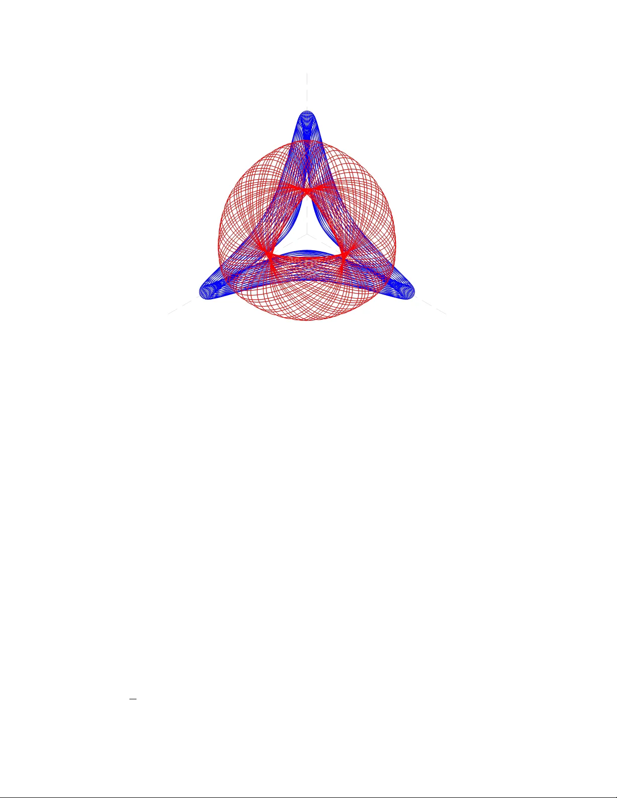
P oincaré Recurr ence, Cycles and Spurious Equilibria in Gradient-Descent-Ascent f or Non-Con vex Non-Conca v e Zero-Sum Games Lampros Flokas ∗ Department of Computer Science Columbia Univ ersity New Y ork, NY 10025 lamflokas@cs.columbia.edu Emmanouil V . Vlatakis-Gkaragkounis ∗ Department of Computer Science Columbia Univ ersity New Y ork, NY 10025 emvlatakis@cs.columbia.edu Georgios Piliouras Engineering Systems and Design Singapore Uni versity of T echnology and Design Singapore georgios@sutd.edu.sg Abstract W e study a wide clas s of non-con ve x non-conca ve min-max games that generalizes ov er standard bilinear zero-sum games. In this class, players control the inputs of a smooth function whose output is being applied to a bilinear zero-sum game. This class of games is motiv ated by the indirect nature of the competition in Generati ve Adversarial Netw orks, where players control the parameters of a neural netw ork while the actual competition happens between the distrib utions that the generator and discriminator capture. W e establish theoretically , that depending on the speciﬁc instance of the problem gradient-descent-ascent dynamics can exhibit a v ariety of behaviors antithetical to con vergence to the g ame theoretically meaningful min-max solution. Speciﬁcally , different forms of recurrent beha vior (including periodicity and Poincaré recurrence) are possible as well as con ver gence to spurious (non-min- max) equilibria for a positi ve measure of initial conditions. At the technical lev el, our analysis combines tools from optimization theory , game theory and dynamical systems. 1 Introduction Min-max optimization is a problem of interest in sev eral communities including Optimization, Game Theory and Machine Learning. In its most general form, gi ven an objectiv e function r : R n × R m → R and we would like to solv e the follo wing problem ( θ θ θ ∗ , φ φ φ ∗ ) = arg min θ θ θ ∈ R n arg max φ φ φ ∈ R m r ( θ θ θ , φ φ φ ) . (1) This problem is much more complicated compared to classical minimization problems, as even understanding under which conditions such a solution is meaning-full is far from tri vial Daskalakis and Panageas [2018], Mai et al. [2017], Oliehoek et al. [2018], Jin et al. [2019]. What is ev en more demanding is understanding what kind of algorithms/dynamics are able to solve this problem when a solution is well deﬁned. ∗ Equal contribution 33rd Conference on Neural Information Processing Systems (NeurIPS 2019), V ancouver , Canada. Recently this problem has attracted rene wed interest moti vated by the adv ent of Generati ve Adv er- sarial Networks (GANs) and their numerous applications Goodfellow et al. [2014], Radford et al. [2016], Isola et al. [2017], Goodfellow et al. [2014], Zhang et al. [2017], Arjovsk y et al. [2017], Ledig et al. [2017], Salimans et al. [2016]. A classical GAN architecture mainly rev olv es around the competition between two players, the generator and the discriminator . On the one hand, the generator aims to train a neural network based generati ve model that can generate high ﬁdelity samples from a target distribution. On the other hand, the discriminator’ s goal is to train a neural network classiﬁer than can distinguish between the samples of the target distrib ution and artiﬁcially generated samples. While one could consider each of the tasks in isolation, it is the competitive interaction between the generator and the discriminator that has lead to the resounding success of GANs. It is the "criticism" from a powerful discriminator that pushes the generator to capture the target distrib ution more accurately and it is the access to high ﬁdelity artiﬁcial samples from a good generator that gives rise to better discriminators. Machine Learning researchers and practitioners hav e tried to formalize this competition using the min-max optimization framework mentioned abo ve with great success Arora et al. [2017], Ma [2018], Ge et al. [2018], Y azıcı et al. [2019]. One of the main limitations of this frame work ho we ver is that to this day ef ﬁciently training GANs can be a notoriously difﬁcult task Salimans et al. [2016], Metz et al. [2017], Mertikopoulos et al. [2018], Kodali et al. [2017]. Addressing this limitation has been the object of interest for a long line work in the recent years Mescheder et al. [2018], Metz et al. [2017], Pfau and V inyals [2016], Radford et al. [2016], T olstikhin et al. [2017], Berthelot et al. [2017], Gulrajani et al. [2017]. Despite the intensiﬁed study , very little is known about efﬁciently solving general min-max optimization problems. Even for the relativ ely simple case of bilinear games, the little results that are known ha ve usually a neg ativ e ﬂav our . For example, the continuous time analogue of standard game dynamics such as gradient-descent-ascent or multiplicati ve weights lead to c yclic or recurrent behavior Piliouras and Shamma [2014], Mertikopoulos et al. [2018] whereas when the y are actually run in discrete-time 2 they lead to di ver gence and chaos Bailey and Piliouras [2018], Cheung and Piliouras [2019], Bailey and Piliouras [2019b]. While positive results for the case of bilinear games exist , like extra-gradient (optimistic) training (Daskalakis et al. [2018], Mertikopoulos et al. [2019a], Daskalakis and Panageas [2019]) and other techniques Balduzzi et al. [2018], Gidel et al. [2019b,a], Abernethy et al. [2019], these results fail to generalize to comple x non-con v ex non-conca ve settings Oliehoek et al. [2018], Lin et al. [2018], Sanjabi et al. [2018]. In fact, for the case of non-con ve x-concav e optimization, game theoretic interpretations of equilibria might not ev en be meaningful Mazumdar and Ratliff [2018], Jin et al. [2019], Adolphs et al. [2019]. In order to shed some light to this intellectually challenging problem, we propose a quite general class of min-max optimization problems that includes bilinear games as well as a wide range of non-con ve x non-concave games. In this class of problems, each player submits its own decision vector just lik e in general min-max optimization problems. Then each decision vector is processed separately by a (potentially dif ferent) smooth function. Each player ﬁnally gets rew arded by plugging in the processed decision vectors to a simple bilinear game. More concretely , there are functions F : R n → R N and G : R m → R M and a matrix U N × M such that r ( θ θ θ , φ φ φ ) = F F F ( θ θ θ ) > U G G G ( φ φ φ ) . (2) W e call the resulting class of problems Hidden Bilinear Games. The moti vation behind the proposed class of gamess is actually the setting of training GANs itself. During the training process of GANs, the discriminator and the generator "submit" the parameters of their corresponding neural network architectures, denoted as θ θ θ and φ φ φ in our problem formulation. Howe v er , deep networks introduce nonlinearities in mapping their parameters to their output space which we capture through the non-con ve x functions F , G . Thus, ev en though hidden bilinear games do not demonstrate the full complexity of modern GAN architectures and training, they manage to capture two of its most pervasi v e properties: i) the indirect competition of the generator and the discriminator and ii) the non-con vex non-concave nature of training GANs . Both features are markedly missing from simple bilinear games. Our results. W e provide, the ﬁrst to our own kno wledge, global analysis of gradient-descent-ascent for a class of non-con ve x non-concav e zero-sum games that by design includes both features of 2 Interestingly , running alternating gradient-descent-ascent in discrete-time results once again in recurrent behavior Baile y et al. [2019]. 2 bilinear zero-sum games as well as of single-agent non-con vex optimization. Our analysis focuses on the (smoother) continuous time dynamics (Section 4,5) b ut we also discuss the implications for discrete time (Section 7). The uniﬁed thread of our results is that gradient-descent-ascent can exhibit a variety of beha viors antithetical to con ver gence to the min-max solution. In fact, con ver gence to a set of parameters that implement the desired min-max solution (as e.g. GANs require), if it actually happens, is more of an accident due to fortuitous system initialization rather than an implication of the adversarial network architecture. Informally , we prove that these dynamics exhibit conservation laws, akin to energy conservation in physics. Thus, in contrast to them making progress over time their natural tendencies is to "cycle" through their parameter space. If the hidden bilinear game U is 2x2 (e.g. Matching Pennies) with an interior Nash equilibrium, then the behavior is typically periodic (Theorem 3). If it is a higher dimensional game (e.g. akin to Rock-Paper-Scissors) then even more complex behavior is possible. Speciﬁcally , the system is formally analogous to Poincaré recurrent systems (e.g. many body problem in physics) (Theorems 6, 7). Due to the non-con ve xity of the operators F , G , the system can actually sometimes get stuck at equilibria, ho we ver , these ﬁxed points may be merely artifacts of the nonlinearities of F , G instead of meaningful solutions to the underline minmax problem U . (Theorem 8). In Section 7, we sho w that mo ving from continuous to discrete time, only enhances the disequilibrium properties of the dynamics. Speciﬁcally , instead of ener gy conserv ation no w energy increases o ver time leading aw ay from equilibrium (Theorem 9), whilst spurious (non-minmax) equilibria are still an issue (Theorem 10). Despite these negati ve results, there are some positi ve news, as at least in some cases we can show that time-av eraging ov er these non-equilibrium trajectories (or equiv alently choosing a distribution of parameters instead of a single set of parameters) can recov er the min- max equilibrium (Theorem 4). T echnically our results combine tools from dynamical systems (e.g. Poincaré recurrence theorem, Poincaré-Bendixson theorem, Liouville’ s theorem) along with tools from game theory and non-con v ex optimization. Understanding the intricacies of GAN training requires broadening our vocab ulary and horizons in terms of what type of long term behaviors are possible and de veloping ne w techniques that can hopefully counter them. The structure of the rest of the paper is as follows. In Section 2 we will present key results from prior work on the problem of min-max optimization. In Section 3 we will present the main mathematical tools for our analysis. Sections 4 through 6 will be de voted to studying interesting special cases of hidden bilinear games. Section 8 will be the conclusion of our work. 2 Related W ork Non-equilibrating dynamics in game theory . Kleinberg et al. [2011] established non-con v ergence for a continuous-time variant of Multiplicati ve W eights Update (MWU), kno wn as the replicator dynamic, for a 2x2x2 game and showed that as a result the system conv erges to states whose social welfare dominates that of all Nash equilibria. Palaiopanos et al. [2017] prov ed the existence of Li-Y orke chaos in MWU dynamics of 2x2 potential games. From the perspective of e volutionary game theory , which typically studies continuous time dynamics, numerous noncon v ergence results are kno wn b ut again typically for small games, e.g., Sandholm [2010]. Piliouras and Shamma [2014] sho ws that replicator dynamics exhibit a speciﬁc type of near periodic behavior in bilinear (network) zero-sum games, which is known as Poincaré recurrence. Recently , Mertikopoulos et al. [2018] generalized these results to more general continuous time v ariants of FTRL dynamics (e.g. gradient-descent-ascent). Cycles arise also in ev olutionary team competition Piliouras and Schulman [2018] as well as in network competition Nagarajan et al. [2018]. T echnically , Piliouras and Schulman [2018] is the closest paper to our own as it studies e v olutionary competition between Boolean functions, howe ver , the dynamics in the two models are different and that paper is strictly focused on periodic systems. The papers in the category of cyclic/recurrent dynamics combine delicate ar guments such as volume preservation and the existence of constants of motions (“energy preservation"). In this paper we provide a wide generalization of these type of results by establishing cycles and recurrence type of behavior for a lar ge class of non-con v ex non-conca ve games. In the case of discrete time dynamics, such as standard gradient-descent-ascent, the system trajectories are ﬁrst order approximations of the abov e motion and these conservation ar guments do not hold exactly . Instead, ev en in bilinear games, 3 Figure 1: T rajectories of a single player using gradient-descent-ascent dynamics for a hidden Rock-Paper -Scissors game with sigmoid activ ations. The dif ferent colors correspond to different ini- tializations of the dynamics. The trajectories exhibit Poincaré recurrence as expected by Theorem 7. the “energy" slo wly increases over time Bailey and Piliouras [2018] implying chaotic div ergence away from equilibrium Cheung and Piliouras [2019]. W e extend such energy increase results to non-linear settings. Learning in zer o-sum games and connections to GANs. Sev eral recent papers ha ve sho wn positi ve results about con ver gence to equilibria in (mostly bilinear) zero-sum games for suitable adapted variants of ﬁrst-order methods and then apply these techniques to Generativ e Adversarial Netw orks (GANs) showing improved performance (e.g. Daskalakis et al. [2018], Daskalakis and Panageas [2019]). Balduzzi et al. [2018] made use of conservation laws of learning dynamics in zero-sum games (e.g. Bailey and Piliouras [2019a]) to develop new algorithms for training GANs that add a ne w component to the vector ﬁeld that aims at minimizing this energy function. Different energy shrinking techniques for con ver gence in GANs (non-conv ex saddle point problems) exploit connections to variational inequalities and emplo y mirror descent techniques with an extra gradient step Gidel et al. [2018], Mertikopoulos et al. [2019a]. Moreover , adding ne gati ve momentum can help with stability in zero-sum games Gidel et al. [2019c]. Game theoretic inspired methods such as time-av eraging work well in practice for a wide range of architectures Y azıcı et al. [2019]. 3 Preliminaries 3.1 Notation V ectors are denoted in boldface x x x, y y y unless otherwise indicated are considered as column vectors. W e use k·k corresponds to denote the ` 2 − norm. For a function f : R d → R we use ∇ f to denote its gradient. For functions of two v ector arguments, f ( x x x, y y y ) : R d 1 × R d 2 → R , we use ∇ x x x f , ∇ y y y f to denote its partial gradient. For the time deriv ativ e we will use the dot accent abbreviation, i.e., ˙ x x x = d dt [ x x x ( t )] . A function f will belong to C r if it is r times continuously differentiable. The term “sigmoid" function refers to σ : R → R such that σ ( x ) = (1 + e − x ) − 1 . Finally , we use P ( · ) , operating ov er a set, to denote its (Lebesgue) measure. 4 3.2 Deﬁnitions Deﬁnition 1 (Hidden Bilinear Zero-Sum Game) . In a hidden bilinear zer o-sum game ther e ar e two players, each one equipped with a smooth function F F F : R n → R N and G G G : R m → R M and a payoff matrix U N × M such that each player inputs its own decision vector θ θ θ ∈ R n and φ φ φ ∈ R m and is trying to maximize or minimize r ( θ θ θ , φ φ φ ) = F F F ( θ θ θ ) > U G G G ( φ φ φ ) r espectively . In this work we will mostly study continuous time dynamics of solutions for the problem of Equation 1 for hidden bilinear zero-sum games b ut we will also make some important connections to discrete time dynamics that are also prev alent in practice. In order to make this distinction clear , let us deﬁne the following terms. Deﬁnition 2 (Continuous T ime Dynamical System) . A system of or dinary differ ential equations ˙ x x x = f ( x x x ) wher e f : R d → R d will be called a continuous time dynamical system. Solutions of the equation f ( x x x ) = 0 ar e called the ﬁxed points of the dynamical system. W e will call f the vector ﬁeld of the dynamical system. In order to understand the properties of continuous time dynamical systems, we will often need to study their behaviour giv en dif ferent initial conditions. This behaviour is captured by the ﬂo w of the dynamical system. More precisely , Deﬁnition 3. If f is Lipsc hitz-continuous, ther e e xists a continuous map Φ( x x x 0 , t ) : R d × R → R d called ﬂow of the dynamical system such that for all x x x 0 ∈ R d we have that Φ( x x x 0 , t ) is the unique solution of the pr oblem { ˙ x x x = f ( x x x ) , x x x (0) = x x x 0 } . W e will r efer to Φ( x x x 0 , t ) as a trajectory or orbit of the dynamical system. In this work we will be mainly study the gradient-descent-ascent dynamics for the problem of Equation 1. The continuous (discrete) time version of the dynamics (with learning rate α ) are based on the following equations: ( CGD A ) :  ˙ θ θ θ = −∇ θ θ θ r ( θ θ θ , φ φ φ ) ˙ φ φ φ = ∇ φ φ φ r ( θ θ θ , φ φ φ )  (DGD A ) :  θ θ θ k +1 = θ θ θ k − α ∇ θ θ θ r ( θ θ θ k , φ φ φ k ) φ φ φ k +1 = φ φ φ k + α ∇ φ φ φ r ( θ θ θ k , φ φ φ k )  A key notion in our analysis is that of (Poincaré) recurrence. Intuitiv ely , a dynamical system is recurrent if, after a sufﬁciently long (b ut ﬁnite) time, almost ev ery state returns arbitrarily close to the system’ s initial state. Deﬁnition 4. A point x ∈ R d is said to be recurr ent under the ﬂow Φ , if for every neighborhood U ⊆ R d of x , ther e e xists an increasing sequence of times t n such that lim n →∞ t n = ∞ and Φ( x , t n ) ∈ U for all n . Mor eover , the ﬂow Φ is called P oincaré recurr ent in non-zer o measur e set A ⊆ R d if the set of the non-r ecurr ent points in A has zero measur e. 4 Cycles in hidden bilinear games with two strategies In this section we will focus on a particular case of hidden biinear games where both the generator and the discriminator play only two strategies. Let U be our zero-sum game and without loss of generality we can assume that there are functions f : R n → [0 , 1] and g : R m → [0 , 1] such that F F F ( θ θ θ ) =  f ( θ θ θ ) 1 − f ( θ θ θ )  U =  u 0 , 0 u 0 , 1 u 1 , 0 u 1 , 1  G G G ( φ φ φ ) =  g ( φ φ φ ) 1 − g ( φ φ φ )  Let us assume that the hidden bi-linear game has a unique mixed Nash equilibrium ( p, q ) : v = u 0 , 0 − u 0 , 1 − u 1 , 0 + u 1 , 1 6 = 0 , q = − u 0 , 1 − u 1 , 1 v ∈ (0 , 1) , p = − u 1 , 0 − u 1 , 1 v ∈ (0 , 1) Then we can write down the equations of gradient-descent-ascent : ( ˙ θ θ θ = − v ∇ f ( θ θ θ )( g ( φ φ φ ) − q ) ˙ φ φ φ = v ∇ g ( φ φ φ )( f ( θ θ θ ) − p ) ) (3) In order to analyze the behavior of this system, we would like to understand the topology of the trajectories of θ θ θ and φ φ φ , at least indi vidually . The following lemma makes a connection between the trajectories of each v ariable in the min-max optimization system of Equation 3 and simple gradient ascent dynamics. 5 Lemma 1. Let k : R d → R be a C 2 function. Let h : R → R be a C 1 function and x x x ( t ) = ρ ( t ) be the unique solution of the dynamical system Σ 1 . Then for the dynamical system Σ 2 the unique solution is z z z ( t ) = ρ ( R t 0 h ( s )d s )  ˙ x x x = ∇ k ( x x x ) x x x (0) = x x x 0  : Σ 1  ˙ z z z = h ( t ) ∇ k ( z z z ) z z z (0) = x x x 0  : Σ 2 By applying the previous result for θ θ θ with k = f and h ( t ) = − v ( g ( φ φ φ ( t )) − q ) , we get that ev en under the dynamics of Equation 3, θ θ θ remains on a trajectory of the simple gradient ascent dynamics with initial condition θ θ θ (0) . This necessarily affects the possible v alues of f and g giv en the initial conditions. Let us deﬁne the sets of values attainable for each initialization. Deﬁnition 5. F or each θ θ θ (0) , f θ θ θ (0) is the set of possible values of f ( θ θ θ ( t )) can attain under gradient ascent dynamics. Similarly , we deﬁne g φ φ φ (0) the corr esponding set for g . What is special about the trajectories of gradient ascent is that along this curve f is strictly increasing (For a detailed e xplanation, reader could check the proof of Theorem 1 in the Appendix) and therefore each point θ θ θ ( t ) in the trajectory has a unique value for f . Therefore ev en in the system of Equation 3, f ( θ θ θ ( t )) uniquely identiﬁes θ θ θ ( t ) . This can be formalized in the next theorem. Theorem 1. F or each θ θ θ (0) , φ φ φ (0) , under the dynamics of Equation 3, ther e are C 1 functions ( X θ θ θ (0) , X φ φ φ (0) ) such that X θ θ θ (0) : f θ θ θ (0) → R n , X φ φ φ (0) : g φ φ φ (0) → R n and θ θ θ ( t ) = X θ θ θ (0) ( f ( t )) , φ φ φ ( t ) = X φ φ φ (0) ( g ( t )) . Equipped with these results, we are able to reduce this complicated dynamical system of θ θ θ and φ φ φ to a planar dynamical system in v olving f and g alone. Lemma 2. If θ θ θ ( t ) and φ φ φ ( t ) ar e solutions to Equation 3 with initial conditions ( θ θ θ (0) , φ φ φ (0)) , then we have that f ( t ) = f ( θ θ θ ( t )) and g ( t ) = g ( φ φ φ ( t )) satisfy the following equations ˙ f = − v k∇ f ( X θ θ θ (0) ( f )) k 2 ( g − q ) ˙ g = v k∇ g ( X φ φ φ (0) ( g )) k 2 ( f − p ) (4) As one can observe both form Equation 3 and Equation 4, ﬁxed points of the gradient-descent-ascent dynamics correspond to either solutions of f ( θ θ θ ) = p and g ( φ φ φ ) = q or stationary points of f and g or ev en some combinations of the aforementioned conditions. Although, all of them are ﬁxed points of the dynamical system, only the former equilibria are game theoretically meaningful. W e will therefore deﬁne a subset of initial conditions for Equation 3 such that con ver gence to game theoretically meaningful ﬁxed points may actually be feasible: Deﬁnition 6. W e will call the initialization ( θ θ θ (0) , φ φ φ (0)) safe for Equation 3 if θ θ θ (0) and φ φ φ (0) ar e not stationary points of f and g r espectively and p ∈ f θ θ θ (0) and q ∈ g φ φ φ (0) . For safe initial conditions we can sho w that gradient-descent-ascent dynamics applied in the class of the hidden bilinear zero-sum game mim ic properties and behaviors of conservati v e/Hamiltonian physical systems Bailey and Piliouras [2019a], like an ideal pendulum or an ideal spring-mass system. In such systems, there is a notion of energy that remains constant over time and hence the system trajectories lie on le vel sets of these functions. T o motiv ate further this intuition, it is easy to check that for the simpliﬁed case where k∇ f k = k∇ g k = 1 the lev el sets correspond to cycles centered at the Nash equilibrium and the system as a whole captures gradient-descent-ascent for a bilinear 2 × 2 zero-sum game (e.g. Matching Pennies). Theorem 2. Let θ θ θ (0) and φ φ φ (0) be safe initial conditions. Then for the system of Equation 3, the following quantity is time-in variant H ( f , g ) = Z f p z − p k∇ f ( X θ θ θ (0) ( z )) k 2 d z + Z g q z − q k∇ g ( X φ φ φ (0) ( z )) k 2 d z The e xistence of this in variant immediately guarantees that Nash Equilibrium ( p, q ) cannot be reached if the dynamical system is not initialized there. T aking advantage of the planarity of the induced system - a necessary condition of Poincaré-Bendixson Theorem - we can prov e that: 6 Theorem 3. Let θ θ θ (0) and φ φ φ (0) be safe initial conditions. Then for the system of Equation 3, the orbit ( θ θ θ ( t ) , φ φ φ ( t )) is periodic. On a positiv e note, we can prove that the time av erages of f and g as well as the time av erages of expected utilities of both players con verge to their Nash equilibrium v alues. Theorem 4. Let θ θ θ (0) and φ φ φ (0) be safe initial conditions and ( P P P , Q Q Q ) =   p 1 − p  ,  q 1 − q   , then for the system of Equation 3 lim T →∞ R T 0 f ( θ θ θ ( t ))d t T = p, lim T →∞ R T 0 r ( θ θ θ ( t ) , φ φ φ ( t ))d t T = P P P > U Q Q Q, lim T →∞ R T 0 g ( φ φ φ ( t ))d t T = q 5 Poincaré r ecurr ence in hidden bilinear games with more strategies In this section we will extend our results by allowing both the generator and the discriminator to play hidden bilinear games with more than tw o strategies. W e will speciﬁcally study the case of hidden bilinear games where each coordinate of the vector v alued functions F and G is controlled by disjoint subsets of the variables θ θ θ and φ φ φ , i.e. θ θ θ =     θ θ θ 1 θ θ θ 2 . . . θ θ θ N     F F F ( θ θ θ ) =     f 1 ( θ θ θ 1 ) f 2 ( θ θ θ 2 ) . . . f N ( θ θ θ N )     φ φ φ =     φ φ φ 1 φ φ φ 2 . . . φ φ φ M     G G G ( φ φ φ ) =     g 1 ( φ φ φ 1 ) g 2 ( φ φ φ 2 ) . . . g M ( φ φ φ M )     (5) where each function f i and g i takes an appropriately sized vector and returns a non-negati ve number . T o account for possible constraints (e.g. that probabilities of each distribution must sum to one), we will incorporate this restriction using Lagrange Multipliers. The resulting problem becomes min θ θ θ ∈ R n ,µ ∈ R max φ φ φ ∈ R m ,λ ∈ R F F F ( θ θ θ ) > U G G G ( φ φ φ ) + λ N X i =1 f i ( θ θ θ i ) − 1 ! + µ   M X i = j g j ( φ φ φ j ) − 1   (6) Writing down the equations of gradient-ascent-descent we get ˙ θ θ θ i = − ∇ f i ( θ θ θ i )   M X j =1 u i,j g j ( φ φ φ j ) + λ   ˙ φ φ φ j = ∇ g j ( φ φ φ j ) N X i =1 u i,j f i ( θ θ θ i ) + µ ! ˙ µ = −   M X j =1 g j ( φ φ φ j ) − 1   ˙ λ = N X i =1 f i ( θ θ θ i ) − 1 ! (7) Once again we can sho w that along the trajectories of the system of Equation 7, θ θ θ i can be uniquely identiﬁed by f i ( θ θ θ i ) giv en θ θ θ i (0) and the same holds for the discriminator . This allows us to construct functions X θ θ θ i (0) and X φ φ φ j (0) just like in Theorem 1. W e can now write down a dynamical system in v olving only f i and g j . Lemma 3. If θ θ θ ( t ) and φ φ φ ( t ) ar e solutions to Equation 7 with initial conditions ( θ θ θ (0) , φ φ φ (0) , λ (0) , µ (0)) , then we have that f i ( t ) = f i ( θ θ θ i ( t )) and g j ( t ) = g j ( φ φ φ j ( t )) satisfy the following equations ˙ f i = −k∇ f i ( X θ θ θ i (0) ( f i )) k 2   M X j =1 u i,j g j + λ   ˙ g j = k∇ g j ( X φ φ φ j (0) ( g j )) k 2 N X i =1 u i,j f i + µ ! (8) Similarly to the previous section, we can deﬁne a notion of safety for Equation 7. Let us assume that the hidden Game has a fully mixed Nash equilibrium ( p p p, q q q ) . Then we can deﬁne Deﬁnition 7. W e will call the initialization ( θ θ θ (0) , φ φ φ (0) , λ (0) , µ (0)) safe for Equation 7 if θ θ θ i (0) and φ φ φ j (0) ar e not stationary points of f i and g j r espectively and p i ∈ f i θ θ θ i (0) and q j ∈ g j φ φ φ j (0) . 7 Theorem 5. Assume that ( θ θ θ (0) , φ φ φ (0) , λ (0) , µ (0)) is a safe initialization. Then ther e exist λ ∗ and µ ∗ such that the following quantity is time in variant: H ( F F F , G G G, λ, µ ) = N X i =1 Z f i p i z − p i k∇ f i ( X θ θ θ i (0) ( z )) k 2 d z + M X j =1 Z g j q j z − q j k∇ g j ( X φ φ φ j (0) ( z )) k 2 d z + Z λ λ ∗ ( z − λ ∗ ) d z + Z µ µ ∗ ( z − µ ∗ ) d z Giv en that e ven our reduced dynamical system has more than tw o state variables we cannot apply the Poincaré-Bendixson Theorem. Instead we can prov e that there exists a one to one dif ferentiable transformation of our dynamical system so that the resulting system becomes di ver gence free. Applying Louville’ s formula, the ﬂo w of the the transformed system is v olume preserving. Combined with the in v ariant of Theorem 5, we can prov e that the v ariables of the transformed system remain bounded. This giv es us the follo wing guarantees Theorem 6. Assume that ( θ θ θ (0) , φ φ φ (0) , λ (0) , µ (0)) is a safe initialization. Then the trajectory under the dynamics of Equation 7 is diffeomoprphic to one tr ajectory of a P oincaré r ecurr ent ﬂow . This result implies that if the corresponding trajectory of the Poincaré recurrent ﬂow is itself recurrent, which almost all of them are, then the trajectory of the dynamics of Equation 7 is also recurrent. This is howe v er not enough to reason about ho w often any of the trajectories of the dynamics of Equation 7 is recurrent. In order to prove that the ﬂo w of Equation 7 is Poincaré recurrent we will make some additional assumptions Theorem 7. Let f i and g j be sigmoid functions. Then the ﬂow of Equation 7 is P oincaré recurr ent. The same holds for all functions f i and g j that are one to one functions and for which all initializations ar e safe. It is worth noting that for the unconstrained v ersion of the pre vious min-max problem we arri ve at the same conclusions/theorems by repeating the abov e analysis without using the Lagrange multipliers. 6 Spurious equilibria In the previous sections we have analyzed the behavior of safe initializations and we hav e proved that they lead to either periodic or recurrent trajectories. For initializations that are not safe for some equilibrium of the hidden g ame, game theoretically interesting ﬁx ed points are not e ven realizable solutions. In fact we can prov e something stronger: Theorem 8. One can construct functions f and g for the system of Equation 3 so that for a positive measur e set of initial conditions the trajectories con verge to ﬁxed points that do not corr espond to equilibria of the hidden game. The main idea behind our theorem is that we can construct functions f and g that have local optima that break the safety assumption. For a careful choice of the v alue of the local optima we can make these ﬁxed points stable and then the Stable Manifold Theorem guarantees that a non zero measure set of points in the vicinity of the ﬁxed point con ver ges to it. Of course the idea of these constructions can be extended to our analysis of hidden games with more strate gies. 7 Discrete T ime Gradient-Ascent-Descent In this section we will discuss the implications of our analysis of continuous time gradient-ascent- descent dynamics on the properties of their discrete time counterparts. In general, the behavior of discrete time dynamical systems can be signiﬁcantly diff erent Li and Y orke [1975], Bailey and Piliouras [2018], Palaiopanos et al. [2017] so it is critical to perform this non-trivial analysis. W e are able to show that the picture of non-equilibriation persists for an interesting class of hidden bilinear games. Theorem 9. Let f i and g j be sigmoid functions. Then for the discretized version of the system of Equation 7 and for safe intializations, function H of Theor em 5 is non-decr easing. 8 An immediate consequence of the abo ve theorem is that the discretized system cannot con v erge to the equlibrium ( p p p, q q q ) if its not initialized there. For the case of non-safe initializations, the conclusions of Theorem 8 persist in this case as well. Theorem 10. One can choose a learning rate α and functions f and g for the discretized version of the system of Equation 3 so that for a positive measur e set of initial conditions the trajectories con ver ge to ﬁxed points that do not corr espond to equilibria of the hidden game. 8 Conclusion In this work, inspired broadly by the structure of the complex competition between generators and discriminators in GANs, we deﬁned a broad class of non-con ve x non-concav e min max optimization games, which we call hidden bilinear zero-sum games. In this setting, we showed that gradient- descent-ascent behavior is considerably more complex than a straightforward con ver gence to the min-max solution that one might at ﬁrst suspect. W e showed that the trajectories ev en for the simplest b ut e vocati ve 2x2 game exhibits cycles. In higher dimensional games, the induced dynamical system could exhibit e ven more complex beha vior like Poincare recurrence. On the other hand, we explored safety conditions whose violation may result in conv ergence to spurious game-theoretically meaningless equilibria. Finally , we show that e ven for a simple but widespread f amily of functions like sigmoids discretizing gradient-descent-ascent can further intensify the disequilibrium phenomena resulting in div ergence a way from equilibrium. As a consequence of this work numerous open problems emer ge; Firstly , extending such recurrence results to more general families of functions, as well as examining possible generalizations to multi- player network zero-sum games are fascinating questions. Recently , there has been some progress in resolving cyclic beha vior in simpler settings by employing dif ferent training algorithms/dynamics (e.g., Daskalakis et al. [2018], Mertikopoulos et al. [2019b], Gidel et al. [2019c]). It would be inter- esting to examine if these algorithms could enhance equilibration in our setting as well. Additionally , the proposed safety conditions shows that a major source of spurious equilibria in GANs could be the bad local optima of the individual neural networks of the discriminator and the generator . Lessons learned from overparametrized neural netw ork architectures that con ver ge to global optima Du et al. [2018] could lead to improved efﬁcienc y in training GANs. Finally , analyzing different simpliﬁcation/models of GANs where provable conv ergence is possible could lead to interesting comparisons as well as to the emer gence of theoretically tractable hybrid models that capture both the hardness of GAN training (e.g. non-con ver gence, cycling, spurious equilibria, mode collapse, etc) as well as their power . Acknowledgements Georgios Piliouras ackno wledges MOE AcRF T ier 2 Grant 2016-T2-1-170, grant PIE-SGP-AI-2018- 01 and NRF 2018 Fellowship NRF-NRFF2018-07. Emmanouil-V asileios Vlatakis-Gkaragkounis was supported by NSF CCF-1563155, NSF CCF-1814873, NSF CCF-1703925, NSF CCF-1763970. Finally this work was supported by the Onassis Foundation - Scholarship ID: F ZN 010-1/2017-2018. References Jacob Abernethy , Ke vin A. Lai, and Andre W ibisono. Last-iterate con v ergence rates for min-max optimization. CoRR , abs/1906.02027, 2019. Leonard Adolphs, Hadi Daneshmand, Aurélien Lucchi, and Thomas Hofmann. Local saddle point optimization: A curvature exploitation approach. In The 22nd International Conference on Artiﬁcial Intelligence and Statistics, AIST A TS 2019, 16-18 April 2019, Naha, Okinawa, Japan , pages 486–495, 2019. URL http://proceedings.mlr.press/v89/adolphs19a.html . Martín Arjovsk y , Soumith Chintala, and Léon Bottou. W asserstein GAN. CoRR , abs/1701.07875, 2017. URL . Sanjeev Arora, Rong Ge, Y ingyu Liang, T engyu Ma, and Y i Zhang. Generalization and equilibrium in generativ e adversarial nets (gans). In Pr oceedings of the 34th International Confer ence on 9 Machine Learning, ICML 2017, Sydne y , NSW , Austr alia, 6-11 August 2017 , pages 224–232, 2017. URL http://proceedings.mlr.press/v70/arora17a.html . James P . Bailey and Georgios Piliouras. Multiplicativ e weights update in zero-sum games. In Pr oceedings of the 2018 ACM Confer ence on Economics and Computation, Ithaca, NY , USA, June 18-22, 2018 , pages 321–338, 2018. doi: 10.1145/3219166.3219235. URL https://doi.org/ 10.1145/3219166.3219235 . James P . Bailey and Georgios Piliouras. Multi-agent learning in network zero-sum games is a hamiltonian system. In 18th International Confer ence on Autonomous Agents and Multiagent Systems (AAMAS) , 2019a. James P Bailey and Georgios Piliouras. Fast and furious learning in zero-sum games: V anishing regret with non-v anishing step sizes. In NeurIPS , 2019b. James P . Bailey and Georgios Piliouras. Multi-agent learning in network zero-sum games is a hamiltonian system. In Pr oceedings of the 18th International Confer ence on A utonomous Agents and MultiAgent Systems, AAMAS ’19, Montr eal, QC, Canada, May 13-17, 2019 , pages 233–241, 2019c. URL http://dl.acm.org/citation.cfm?id=3331698 . James P . Bailey , Gauthier Gidel, and Georgios Piliouras. Finite regret and cycles with ﬁxed step-size via alternating gradient descent-ascent. CoRR , abs/1907.04392, 2019. David Balduzzi, Sebastien Racaniere, James Martens, Jakob Foerster , Karl T uyls, and Thore Graepel. The mechanics of n-player differentiable games. In International Conference on Machine Learning , pages 363–372, 2018. Iv ar Bendixson. Sur les courbes déﬁnies par des équations dif férentielles. Acta Math. , 24:1–88, 1901. doi: 10.1007/BF02403068. URL https://doi.org/10.1007/BF02403068 . David Berthelot, T om Schumm, and Luke Metz. BEGAN: boundary equilibrium generati ve adversar - ial networks. CoRR , abs/1703.10717, 2017. URL . Y un Kuen Cheung and Georgios Piliouras. V ortices instead of equilibria in minmax optimization: Chaos and butterﬂy ef fects of online learning in zero-sum games. In COLT , 2019. Constantinos Daskalakis and Ioannis Panageas. The limit points of (optimistic) gradient descent in min-max optimization. In Advances in Neural Information Pr ocessing Systems 31: Annual Confer ence on Neur al Information Pr ocessing Systems 2018, NeurIPS 2018, 3-8 December 2018, Montréal, Canada. , pages 9256–9266, 2018. URL http://papers.nips.cc/paper/ 8136- the- limit- points- of- optimistic- gradient- descent- in- min- max- optimization . Constantinos Daskalakis and Ioannis Panageas. Last-iterate con ver gence: Zero-sum games and con- strained min-max optimization. In 10th Innovations in Theoretical Computer Science Confer ence , ITCS 2019, January 10-12, 2019, San Die go, California, USA , pages 27:1–27:18, 2019. doi: 10.4230/LIPIcs.ITCS.2019.27. URL https://doi.org/10.4230/LIPIcs.ITCS.2019.27 . Constantinos Daskalakis, Andre w Ilyas, V asilis Syrgkanis, and Haoyang Zeng. Training gans with optimism. In 6th International Confer ence on Learning Repr esentations, ICLR 2018, V ancouver , BC, Canada, April 30 - May 3, 2018, Confer ence T rac k Pr oceedings , 2018. URL https:// openreview.net/forum?id=SJJySbbAZ . Simon S. Du, Jason D. Lee, Haochuan Li, Liwei W ang, and Xiyu Zhai. Gradient descent ﬁnds global minima of deep neural networks. CoRR , abs/1811.03804, 2018. URL 1811.03804 . Hao Ge, Y in Xia, Xu Chen, Randall Berry , and Y ing W u. Fictitious GAN: training gans with historical models. In Computer V ision - ECCV 2018 - 15th European Confer ence, Munich, Germany , September 8-14, 2018, Pr oceedings, P art I , pages 122–137, 2018. doi: 10.1007/ 978- 3- 030- 01246- 5\_8. URL https://doi.org/10.1007/978- 3- 030- 01246- 5_8 . Gauthier Gidel, Hugo Berard, P ascal V incent, and Simon Lacoste-Julien. A variational inequality perspectiv e on generati ve adv ersarial nets. CoRR , abs/1802.10551, 2018. URL http://arxiv. org/abs/1802.10551 . 10 Gauthier Gidel, Hugo Berard, Gaëtan V ignoud, Pascal V incent, and Simon Lacoste-Julien. A variational inequality perspectiv e on generativ e adversarial networks. In ICLR , 2019a. URL https://openreview.net/forum?id=r1laEnA5Ym . Gauthier Gidel, Reyhane Askari Hemmat, Mohammad Pezeshki, Gabriel Huang, Rémi Lepriol, Simon Lacoste-Julien, and Ioannis Mitliagkas. Negativ e momentum for improved game dynamics. In AIST A TS , 2019b. Gauthier Gidel, Reyhane Askari Hemmat, Mohammad Pezeshki, Rémi Le Priol, Gabriel Huang, Simon Lacoste-Julien, and Ioannis Mitliagkas. Negativ e momentum for improved game dynamics. In The 22nd International Conference on Artiﬁcial Intelligence and Statistics, AIST A TS 2019, 16-18 April 2019, Naha, Okinawa, J apan , pages 1802–1811, 2019c. URL http://proceedings. mlr.press/v89/gidel19a.html . Ian J. Goodfello w , Jean Pouget-Abadie, Mehdi Mirza, Bing Xu, David W arde-Farley , Sherjil Ozair , Aaron C. Courville, and Y oshua Bengio. Generativ e adversarial nets. In Advances in Neural Information Pr ocessing Systems 27: Annual Confer ence on Neural Information Pr ocessing Systems 2014, December 8-13 2014, Montreal, Quebec, Canada , pages 2672–2680, 2014. URL http: //papers.nips.cc/paper/5423- generative- adversarial- nets . Ishaan Gulrajani, Faruk Ahmed, Martín Arjovsky , V incent Dumoulin, and Aaron C. Courville. Improv ed training of wasserstein gans. In Advances in Neural Information Pr ocessing Sys- tems 30: Annual Confer ence on Neural Information Pr ocessing Systems 2017, 4-9 December 2017, Long Beach, CA, USA , pages 5767–5777, 2017. URL http://papers.nips.cc/paper/ 7159- improved- training- of- wasserstein- gans . Phillip Isola, Jun-Y an Zhu, Tinghui Zhou, and Alex ei A. Efros. Image-to-image translation with conditional adversarial networks. In 2017 IEEE Conference on Computer V ision and P attern Recognition, CVPR 2017, Honolulu, HI, USA, J uly 21-26, 2017 , pages 5967–5976, 2017. doi: 10.1109/CVPR.2017.632. URL https://doi.org/10.1109/CVPR.2017.632 . Chi Jin, Praneeth Netrapalli, and Michael I. Jordan. Minmax optimization: Stable limit points of gradient descent ascent are locally optimal. CoRR , abs/1902.00618, 2019. URL http://arxiv. org/abs/1902.00618 . Robert D. Kleinberg, Katrina Ligett, Georgios Piliouras, and Éva T ardos. Beyond the nash equi- librium barrier . In Innovations in Computer Science - ICS 2010, Tsinghua University , Beijing, China, J anuary 7-9, 2011. Pr oceedings , pages 125–140, 2011. URL http://conference.iiis. tsinghua.edu.cn/ICS2011/content/papers/15.html . Nav een K odali, Jacob D. Abernethy , James Hays, and Zsolt Kira. On con ver gence and stability of gans. CoRR , abs/1705.07215, 2017. URL . Christian Ledig, Lucas Theis, Ferenc Huszar , Jose Caballero, Andrew Cunningham, Alejandro Acosta, Andrew P . Aitken, Alykhan T ejani, Johannes T otz, Zehan W ang, and W enzhe Shi. Photo-realistic single image super -resolution using a generati ve adv ersarial network. In 2017 IEEE Confer ence on Computer V ision and P attern Recognition, CVPR 2017, Honolulu, HI, USA, J uly 21-26, 2017 , pages 105–114, 2017. doi: 10.1109/CVPR.2017.19. URL https://doi.org/10.1109/CVPR. 2017.19 . T ien-Y ien Li and James A. Y orke. Period three implies chaos. The American Mathematical Monthly , 82(10):985–992, 1975. Qihang Lin, Mingrui Liu, Hassan Raﬁque, and Tianbao Y ang. Solving weakly-conv ex-weakly- concav e saddle-point problems as weakly-monotone v ariational inequality . CoRR , abs/1810.10207, 2018. URL . T engyu Ma. Generalization and equilibrium in generativ e adversarial nets (gans) (in vited talk). In Pr oceedings of the 50th Annual A CM SIGA CT Symposium on Theory of Computing, ST OC 2018, Los Angeles, CA, USA, June 25-29, 2018 , page 2, 2018. doi: 10.1145/3188745.3232194. URL https://doi.org/10.1145/3188745.3232194 . 11 T ung Mai, Ioannis Panageas, W ill Ratcliff, V ijay V . V azirani, and Peter Y unker . Rock-paper- scissors, differential g ames and biological div ersity . CoRR , abs/1710.11249, 2017. URL http: //arxiv.org/abs/1710.11249 . Eric Mazumdar and Lillian J. Ratlif f. On the con v ergence of gradient-based learning in continuous games. CoRR , abs/1804.05464, 2018. URL . Panayotis Mertikopoulos, Christos H. Papadimitriou, and Geor gios Piliouras. Cycles in adversarial regularized learning. In Pr oceedings of the T wenty-Ninth Annual A CM-SIAM Symposium on Dis- cr ete Algorithms, SOD A 2018, New Orleans, LA, USA, J anuary 7-10, 2018 , pages 2703–2717, 2018. doi: 10.1137/1.9781611975031.172. URL https://doi.org/10.1137/1.9781611975031. 172 . Panayotis Mertikopoulos, Bruno Lecouat, Houssam Zenati, Chuan-Sheng Foo, V ijay Chandrasekhar, and Geor gios Piliouras. Optimistic mirror descent in saddle-point problems: Going the e xtra (gradi- ent) mile. In 7th International Confer ence on Learning Representations, ICLR 2019, New Orleans, LA, USA, May 6-9, 2019 , 2019a. URL https://openreview.net/forum?id=Bkg8jjC9KQ . Panayotis Mertikopoulos, Bruno Lecouat, Houssam Zenati, Chuan-Sheng Foo, V ijay Chandrasekhar, and Georgios Piliouras. Optimistic mirror descent in saddle-point problems: Going the extra(- gradient) mile. In ICLR , 2019b. URL https://openreview.net/forum?id=Bkg8jjC9KQ . Lars M. Mescheder , Andreas Geiger , and Sebastian No wozin. Which training methods for gans do actually conv erge? In Pr oceedings of the 35th International Confer ence on Machine Learning, ICML 2018, Stoc kholmsmässan, Stockholm, Sweden, J uly 10-15, 2018 , pages 3478–3487, 2018. URL http://proceedings.mlr.press/v80/mescheder18a.html . Luke Metz, Ben Poole, David Pfau, and Jascha Sohl-Dickstein. Unrolled generative adversarial networks. In 5th International Conference on Learning Repr esentations, ICLR 2017, T oulon, F rance, April 24-26, 2017, Conference T rac k Pr oceedings , 2017. URL https://openreview. net/forum?id=BydrOIcle . Sai Ganesh Nagarajan, Sameh Mohamed, and Georgios Piliouras. Three body problems in ev olu- tionary game dynamics: Conv ergence, periodicity and limit cycles. In Pr oceedings of the 17th International Confer ence on A utonomous Agents and MultiAgent Systems, AAMAS 2018, Stock- holm, Sweden, J uly 10-15, 2018 , pages 685–693, 2018. URL http://dl.acm.org/citation. cfm?id=3237485 . Frans A. Oliehoek, Rahul Sav ani, Jose Gallego-Posada, Elise v an der Pol, and Roderich Groß. Beyond local nash equilibria for adversarial networks. CoRR , abs/1806.07268, 2018. URL http://arxiv.org/abs/1806.07268 . Gerasimos Palaiopanos, Ioannis Panageas, and Georgios Piliouras. Multiplicativ e weights update with constant step-size in congestion games: Con ver gence, limit cycles and chaos. In Advances in Neural Information Pr ocessing Systems 30: Annual Confer- ence on Neural Information Pr ocessing Systems 2017, 4-9 December 2017, Long Beach, CA, USA , pages 5872–5882, 2017. URL http://papers.nips.cc/paper/ 7169- multiplicative- weights- update- with- constant- step- size- in- congestion- games- convergence- lim it- c ycles- and- chaos . Lawrence Perko. Differ ential Equations and Dynamical Systems . Springer , 3nd. edition, 1991. David Pf au and Oriol V inyals. Connecting generati ve adversarial netw orks and actor-critic methods. CoRR , abs/1610.01945, 2016. URL . Georgios Piliouras and Leonard J. Schulman. Learning dynamics and the co-ev olution of competing sexual species. In 9th Innovations in Theor etical Computer Science Confer ence, ITCS 2018, J anuary 11-14, 2018, Cambridge , MA, USA , pages 59:1–59:3, 2018. doi: 10.4230/LIPIcs.ITCS. 2018.59. URL https://doi.org/10.4230/LIPIcs.ITCS.2018.59 . Georgios Piliouras and Jeff S. Shamma. Optimization despite chaos: Con ve x relaxations to com- plex limit sets via poincaré recurrence. In Proceedings of the T wenty-F ifth Annual ACM-SIAM Symposium on Discr ete Algorithms, SOD A 2014, P ortland, Ore gon, USA, January 5-7, 2014 , pages 861–873, 2014. doi: 10.1137/1.9781611973402.64. URL https://doi.org/10.1137/1. 9781611973402.64 . 12 H. Poincaré. Sur le problème des trois corps et les équations de la dynamique. Acta Math , 13:1–270, 1890. H Poincaré. Sur le problème des trois corps et les équations de la dynamique. Acta Math. , 13:1, 01 1890. Alec Radford, Luke Metz, and Soumith Chintala. Unsupervised representation learning with deep con volutional generative adversarial networks. In 4th International Confer ence on Learning Repr esentations, ICLR 2016, San J uan, Puerto Rico, May 2-4, 2016, Confer ence T rack Pr oceedings , 2016. URL . T im Salimans, Ian J. Goodfello w , W ojciech Zaremba, V icki Cheung, Alec Radford, and Xi Chen. Improv ed techniques for training gans. In Advances in Neural Information Pr ocessing Sys- tems 29: Annual Confer ence on Neural Information Pr ocessing Systems 2016, December 5-10, 2016, Bar celona, Spain , pages 2226–2234, 2016. URL http://papers.nips.cc/paper/ 6125- improved- techniques- for- training- gans . W illiam H. Sandholm. P opulation Games and Evolutionary Dynamics . MIT Press, 2010. Maziar Sanjabi, Meisam Razaviyayn, and Jason D. Lee. Solving non-con ve x non-concave min- max games under polyak-łojasiewicz condition. CoRR , abs/1812.02878, 2018. URL http: //arxiv.org/abs/1812.02878 . Michael Shub . Global Stability of Dynamical Systems . Springer-V erlag, 1987. Ilya O. T olstikhin, Sylvain Gelly , Oli vier Bousquet, Carl-Johann Simon-Gabriel, and Bernhard Schölkopf. Adagan: Boosting generative models. In Advances in Neural Information Pr ocessing Systems 30: Annual Confer ence on Neural Information Pr ocessing Systems 2017, 4-9 December 2017, Long Beach, CA, USA , pages 5424–5433, 2017. URL http://papers.nips.cc/paper/ 7126- adagan- boosting- generative- models . Y asin Y azıcı, Chuan-Sheng Foo, Stefan Winkler , Kim-Hui Y ap, Georgios Piliouras, and V ijay Chandrasekhar . The unusual effecti veness of a veraging in gan training. In ICLR , 2019. Han Zhang, T ao Xu, and Hongsheng Li. Stackgan: T e xt to photo-realistic image synthesis with stacked generativ e adversarial networks. In IEEE International Confer ence on Computer V ision, ICCV 2017, V enice, Italy , October 22-29, 2017 , pages 5908–5916, 2017. doi: 10.1109/ICCV .2017.629. URL https://doi.org/10.1109/ICCV.2017.629 . 13 P oincaré Recurr ence, Cycles and Spurious Equilibria in Gradient-Descent-Ascent f or Non-Con vex Non-Conca v e Zero-Sum Games Supplementary Material A Background in dynamical systems A.1 Poincaré-Bendixson Theor em The Poincaré-Bendixson theorem is a po werful theorem that implies that two-dimensional systems cannot exhibit chaos. Effecti vely , the limit behavior is either going to be an equilibrium, a periodic orbit, or a closed loop, punctuated by one (or more) ﬁxed points. Formally , we have: Theorem 11 (Poincaré-Bendixson Theorem Bendixson [1901]) . Given a differ entiable r eal dynami- cal system deﬁned on an open subset of the plane, then e very non-empty compact ω -limit set of an orbit, which contains only ﬁnitely many ﬁxed points, is either a ﬁxed point, a periodic orbit, or a connected set composed of a ﬁnite number of ﬁxed points together with homoclinic and heter oclinic orbits connecting these. A.2 Liouville’ s f ormula and Poincaré r ecurrence In order to study the ﬂows of dynamical systems in higher dimensions, one needs to understand more about the behaviour of the ﬂo w Φ both in time and space. An important property is the ev olution of the volume of Φ over time: Theorem 12 (Liouville’ s formula) . Let Φ be the ﬂow of a dynamical system with vecor ﬁeld f . Given any measurable set A , let A ( t ) = Φ( A, t ) and its volume be v ol[ A ( t )] = R A ( t ) d x x x . Then we have that d v ol[ A ( t )] d t = Z A ( t ) div[ f ( x x x )]d x x x An interesting class of dynamical systems are those whose vector ﬁelds have zero diver gence ev erywhere. Liouville’ s formula tri vially implies that the volume of the ﬂow is preserved in such systems. This is an important tool for proving that a ﬂo w of a dynamical system is Poincaré recurrent. Theorem 13 (Poincaré Recurrence Theorem (version 1) [Poincaré, 1890]) . Let ( X, Σ , µ ) be a ﬁnite measur e space and let f : X → X be a measur e-pr eserving tr ansformation. Then, for any E ∈ Σ , the set of those points x of E such that f n ( x ) / ∈ E for all n > 0 has zer o measur e. That is, almost every point of E returns to E . In fact, almost every point r eturns inﬁnitely often. Namely , P ( { x ∈ E : ∃ N such that f n ( x ) / ∈ E for all n > N } ) = 0 . Poincaré [1890] prov ed that in certain systems almost all trajectories return arbitrarily close to their initial position inﬁnitely often. Indeed, let f : X → X be a measure-preserving transformation, { U n : n ∈ N } be a basis of open sets for the bounded subset X ⊂ R d , and for each n deﬁne U n 0 = { x ∈ U n : ∀ n ≥ 1 , f n ( x ) 6∈ U n } . Notice that such basis exists since R n is a second- countable Hausdorff space. From the initial theorem we know that P ( U n 0 ) = 0 . Let U = ∪ n ∈ N U n 0 . Then P ( U ) = 0 . W e assert that if x ∈ X \ U then x is recurrent. In fact, giv en a neighborhood U of x , there is a basic neighborhood U n such that { x } ⊂ U n ⊂ U , and since x 6∈ U we hav e that x ∈ U n \ U n 0 which by deﬁnition of U n 0 means that there e xists n ≥ 1 such that f n ( x ) ∈ U n ⊂ U . Thus x is recurrent. Therefore, for the rest of the paper , we will use the following version which is common in dynamical systems nomenclature. 14 Theorem 14 (Poincaré Recurrence Theorem (dynamical system version)) . P oincaré [1890] If a ﬂow Φ : R n × R → R n pr eserves volume and has only orbits on a bounded subset D of R n then almost eac h point in D is r ecurr ent, i.e for every open neighborhood U of x ther e e xists an incr easing sequence of times t n such that lim n →∞ t n = ∞ and Φ( x , t n ) ∈ U for all n . A.3 Additional Deﬁnitions Deﬁnition 8 (Differomorphism, Perk o [1991]) . Let U, V be manifolds. A map f : U → V is called a diffeomorphism if f carries U onto V and also both f and f − 1 ar e smooth. Deﬁnition 9 (T opological conjugacy , Perko [1991]) . T wo ﬂows Φ t : A → A and Ψ t : B → B ar e conjugate if ther e exists a homeomorphism g : A → B such that ∀ x x x ∈ A, t ∈ R : g (Φ t ( x x x )) = Ψ t ( g ( x x x )) Furthermor e, two ﬂows Φ t : A → A and Ψ t : B → B ar e diffeomorphic if ther e exists a dif feomor - phism g : A → B such that ∀ x x x ∈ A, t ∈ R : g (Φ t ( x x x )) = Ψ t ( g ( x x x )) . If two ﬂows ar e diffeomorphic, then their vector ﬁelds ar e r elated by the derivative of the conjugacy . That is, we get pr ecisely the same r esult that we would have obtained if we simply tr ansformed the coor dinates in their differ ential equations Deﬁnition 10 ( ( α, ω ) -limit set, Perko [1991]) . Let Φ( x x x 0 , · ) be the ﬂow of an autonomous dynamical system ˙ pmbx = f ( x x x ) . Then ω ( x 0 x 0 x 0 ) = { x x x : for all T and all  > 0 ther e exists t > T such that | Φ( x 0 x 0 x 0 , t ) − x x x | <  } α ( x 0 x 0 x 0 ) = { x x x : for all T and all  > 0 ther e exists t < T such that | Φ( x 0 x 0 x 0 , t ) − x x x | <  } Equivalently , ω ( x 0 x 0 x 0 ) = { x x x : ther e exists an unbounded, incr easing sequence { t k } such that lim k →∞ Φ( t k , x 0 x 0 x 0 ) = x x x } α ( x 0 x 0 x 0 ) = { x x x : ther e exists an unbounded, decr easing sequence { t k } such that lim k →∞ Φ( t k , x 0 x 0 x 0 ) = x x x } Lemma 4 (Recurrence and Conjugacy Mertik opoulos et al. [2018]) . Let Φ t : A → A and Ψ t : B → B be conjugate ﬂows and γ be the diffeomorphism which connects them. Then a point x x x ∈ V is r ecurr ent for Φ if and only if γ ( x x x ) ∈ γ ( V ) is r ecurr ent for Ψ . Pr oof. W e will ﬁrst prov e the if direction. Let’ s take any open neighborhood U ⊆ V around x x x . Using the dif feomorphism, there is a unique γ ( U ) ⊆ γ ( V ) and additionally since U is open γ ( U ) is also open. Obviously , γ ( x x x ) ∈ γ ( U ) . Thus, if γ ( x x x ) is recurrent there is an unbounded increasing sequence of moments t n such that Ψ( γ ( x x x ) , t n ) ∈ γ ( U ) . This is equi valent with the fact that there is an unbounded increasing sequence of moments t n such that γ − 1 (Ψ( γ ( x x x ) , t n )) ∈ γ − 1 ( γ ( U )) . Using the basic property of topological conjugacy , we have that Φ( x x x, t n ) = γ − 1 (Ψ( γ ( U ) , t n )) . Thus, for t n we hav e that Φ( x x x, t n ) ∈ U. It follows that x x x is also recurrent for Φ . The result for the opposite direction follows immediately by using the in verse map. 15 A.4 Stable Manifold Theor ems Theorem 15 (Stable Manifold Theorem for Continuous T ime Dynamical Systems p.120 Perko [1991]) . Let E be an open subset of R n containing the origin, let f ∈ C 1 ( E ) , and let φ t be the ﬂow of the nonlinear system ˙ x x x = f ( x x x ) . Suppose that f ( 0 ) = 0 and that D f ( O ) has k eigen values with ne gative r eal part and n − k eigen values with positive r eal part. Then there e xists a k -dimensional differ entiable manifold S tangent to the stable subspace E s of the linear system ˙ x x x = D f ( 0 ) x x x at 0 such that for all t ≥ 0 , φ t ( S ) ⊆ S and for all x x x 0 ∈ S : lim t →∞ φ t ( x x x 0 ) = 0 and ther e e xists an n − k dimensional differ entiable manifold U tangent to the unstable subspace E u of the linear system ˙ x x x = D f ( 0 ) x x x at 0 such that for all t ≤ 0 , φ t ( U ) ⊆ U and for all x x x 0 ∈ U : lim t →−∞ φ t ( x x x 0 ) = 0 Theorem 16 (Center and Stable Manifolds, p. 65 of Shub [1987]) . Let p p p be a ﬁxed point for the C r local diffeomorphism h : U → R n wher e U ⊂ R n is an open neighborhood of p p p in R n and r ≥ 1 . Let E s ⊕ E c ⊕ E u be the in variant splitting of R n into gener alized eigenspaces of D h ( p p p ) 3 corr esponding to eigen values of absolute value less than one, equal to one, and gr eater than one. T o the D h ( p p p ) in variant subspace E s ⊕ E c ther e is an associated local h in variant C r embedded disc W sc loc of dimension dim ( E s ⊕ E c ) , and ball B around p p p such that: h ( W sc loc ) ∩ B ⊂ W sc loc . If h n ( x x x ) ∈ B for all n ≥ 0 , then x x x ∈ W sc loc . A.5 Regular V alue Theorem Deﬁnition 11. Let f : U → V be a smooth map between same dimensional manifolds. W e denote that x ∈ U is a re gular point if the derivative is nonsingular . y ∈ V is called a regular value if f − 1 ( y ) contains only re gular points. If the derivative is singular , then x is called a critical point . W e also say y ∈ V is a critical value if y is not a r e gular value. Theorem 17 (Regular V alue Theorem) . If y ∈ Y is a r e gular value of f : X → Y then f − 1 ( y ) is a manifold of dimension n − m , since dim ( X ) = n and dim ( Y ) = m . 3 Jacobian of h ev aluated at p p p . 16 B Omitted Proofs of Section 4 W arm up: Cycles in hidden bilinear games with two strategies In this ﬁrst section, we show a ke y technical lemma which will be used in many dif ferent parts of our proof. More speciﬁcally , it shows ho w someone can deriv e the solution for a non-autonomous system via a conjugate autonomous dynamical system. The main intuition is that if the non-autonomous term is multiplicati ve and common across all terms of a vector ﬁeld then it dictates the magnitude of the vector ﬁeld (the speed of the motion), but does not affect directionality other than mo ving backwards or forw ards along the same trajectory . Lemma 5 (Restated Lemma 1) . Let k : R d → R be a C 2 function. Let h : R → R be a C 1 function and x x x ( t ) = ρ ( t ) be the unique solution of the dynamical system Σ 1 . Then for the dynamical system Σ 2 the unique solution is z z z ( t ) = ρ ( R t 0 h ( s )d s )  ˙ x x x = ∇ k ( x x x ) x x x (0) = x x x 0  : Σ 1  ˙ z z z = h ( t ) ∇ k ( z z z ) z z z (0) = x x x 0  : Σ 2 Pr oof. Firstly , notice that it holds ρ (0) = x x x 0 and ˙ ρ = ∇ k ( ρ ) , since ρ is the unique solution of Σ 1 It is easy to check that: z z z (0) = ρ ( Z 0 0 h ( s )d s ) = ρ (0) = x x x 0 ˙ z z z = ∇ ρ ( Z t 0 h ( s )d s ) × Z t 0 h ( s )d s = ∇ ρ ( Z t 0 h ( s )d s ) h ( t ) The next proposition states that initial condition ( θ θ θ (0) , φ φ φ (0)) as well as { f ( t ) , g ( t ) } ∞ t =0 are sufﬁcient to deriv e the complete system state of Continuous GD A ( θ θ 0 ( t ) , φ φ 0 ( t )) . The importance of the belo w theorem arises when someone takes into consideration periodicity and recurrence phenomena. Due to the existence of mapping ( f ( t ) , g ( t )) to a unique ( θ θ θ ( t ) , φ φ φ ( t )) giv en some initial condition ( θ θ θ (0) , φ φ φ (0)) , any periodic or recurrent beha vior of ( f ( t ) , g ( t )) e xtends to the system trajectories. Theorem 18 (Restated Theorem 1) . F or each θ θ θ (0) , φ φ φ (0) , under the dynamics of Equation 3, ther e ar e C 1 functions ( X θ θ θ (0) , X φ φ φ (0) ) such that X θ θ θ (0) : f θ θ θ (0) → R n , X φ φ φ (0) : g φ φ φ (0) → R n and θ θ θ ( t ) = X θ θ θ (0) ( f ( t )) , φ φ φ ( t ) = X φ φ φ (0) ( g ( t )) . Pr oof. Let us ﬁrst study a simpler dynamical system (Σ ∗ ) with unique solution of γ θ θ θ (0) ( t ) . (Σ ∗ ) ≡  ˙ θ θ θ = ∇ f ( θ θ θ ) θ θ θ (0) = θ θ θ 0  It is easy to observe that: ˙ f = ∇ f ( θ θ θ ) ˙ θ θ θ = k∇ f ( θ θ θ ) k 2 If x x x 0 is a stationary point of f then the trajectory is a single point and the theorem holds trivially . If x x x 0 is not a stationary point of f , f continuously increases along the trajectory of the dynamical system. Therefore A θ θ θ (0) ( t ) = f ( γ x x x 0 ( t )) is an increasing function and therefore in vertible. Let us call A − 1 θ θ θ (0) ( f ) the inv erse. Let’ s recall now the dynamical system of our interest ( Equation 3 ) CGD A : ( ˙ θ θ θ = − v ∇ f ( θ θ θ )( g ( φ φ φ ) − q ) ˙ φ φ φ = v ∇ g ( φ φ φ )( f ( θ θ θ ) − p ) ) 17 and more precisely to the θ θ θ -part of the system,i.e (Σ) ≡  ˙ θ θ θ = − v ∇ f ( θ θ θ )( g ( φ φ φ ) − q ) θ θ θ (0) = θ θ θ 0  Applying Lemma 5 for the ﬁrst equation with h ( t ) = − v ( g ( φ φ φ ( t )) − q ) , we hav e that the solution of the dynamical system (Σ) is ψ θ θ θ (0) ( t ) = γ θ θ θ (0) ( Z t 0 h ( s )d s | {z } H ( t ) ) = γ θ θ θ (0) ( H ( t )) Thus it holds f ( ψ θ θ θ (0) ( t )) = f ( γ θ θ θ (0) ( H ( t ))) = A θ θ θ (0) ( H ( t )) or equiv alently H ( t ) = A − 1 θ θ θ (0) ( f ( ψ θ θ θ (0) ( t ))) Plug in back to the deﬁnition of the solution, clearly we hav e that : ψ θ θ θ (0) ( t ) = γ θ θ θ (0) ( A − 1 θ θ θ (0) ( f ( ψ θ θ θ (0) ( t )))) Therefore for X θ θ θ (0) ( f ) = γ θ θ θ (0) ◦ A − 1 θ θ θ (0) ( f ) , which is C 1 as composition of C 1 functions, the theorem holds. W e can perform the equiv alent analysis for the φ φ φ (0) and g and prove that for each φ φ φ (0) , under the dynamics Continuous GD A (Equation 3), there is a C 1 function X φ φ φ (0) : g φ φ φ (0) → R n such that φ φ φ ( t ) = X φ φ φ (0) ( g ( t )) . Notice that the domains of the aforementioned functions are in fact either singleton points or open intervals. This will be important when we study the safety of initial conditions. Lemma 6 (Properties of f θ θ θ (0) ) . If θ θ θ (0) is a stationary point of f , then f θ θ θ (0) consists only of a single number . Otherwise, f θ θ θ (0) is an open interval. Pr oof. If θ θ θ (0) is a ﬁxed point then for the gradient ascent dynamics θ θ θ ( t ) = θ θ θ (0) and therefore the Theorem holds trivially . On the other hand, in Theorem 1 we argued that f ( θ θ θ ( t )) is a continuous and strictly increasing function so it should map ( −∞ , ∞ ) to an open set and thus the theorem holds. Obviously we can pro ve an equi v alent theorem for g . 18 Having established the informational equiv alence between the parameter and functional space, we are ready to derive the induced dynamics of the distribution with which two players participate into the game. Lemma 7 (Restated Lemma 2) . If θ θ θ ( t ) and φ φ φ ( t ) ar e solutions to Equation 3 with initial conditions ( θ θ θ (0) , φ φ φ (0)) , then we have that f ( t ) = f ( θ θ θ ( t )) and g ( t ) = g ( φ φ φ ( t )) satisfy the following equations ˙ f = − v k∇ f ( X θ θ θ (0) ( f )) k 2 ( g − q ) ˙ g = v k∇ g ( X φ φ φ (0) ( g )) k 2 ( f − p ) Pr oof. Applying chain rule and the deﬁnition of Continuous GD A (Equation 3) we can see that :  ˙ f = ∇ f ( θ θ θ ( t )) ˙ θ θ θ ( t ) ˙ g = ∇ g ( φ φ φ ( t )) ˙ φ φ φ ( t )  ⇔  ˙ f = − v k∇ f ( θ θ θ ( t )) k 2 2 ( g ( φ φ φ ( t )) − q ) ˙ g = v k∇ g ( φ φ φ ( t )) k 2 2 ( f ( θ θ θ ( t )) − p )  Finally using Theorem 1 we get:  ˙ f = − v k∇ f ( X θ θ θ (0) ( f ( t ))) k 2 2 ( g ( φ φ φ ( t )) − q ) ˙ g = v k∇ g ( X φ φ φ (0) ( g ( t ))) k 2 2 ( f ( θ θ θ ( t )) − p )  Finally , we establish that the above 2-dimensional system that couples f , g together is akin to a conservati ve system that preserves an energy-lik e function. Under the safety conditions, the proposed in v ariant is both well-deﬁned and equipped with interesting properties. It is easy to check that it can play the role of a pseudometric around the Nash Equilibrium of the hidden bilinear game. Theorem 19 (Restated Theorem 2) . Let θ θ θ (0) and φ φ φ (0) be safe initial conditions. Then for the system of Equation 3, the following quantity is time-in variant H ( f , g ) = Z f p z − p k∇ f ( X θ θ θ (0) ( z )) k 2 d z + Z g q z − q k∇ g ( X φ φ φ (0) ( z )) k 2 d z Pr oof. Firstly , one should notice that since θ θ θ (0) and φ φ φ (0) are safe initial conditions, H ( f , g ) is well deﬁned when f , g follows the dynamics Continuous-GD A. W e will examine the deriv ati ve of the proposed in v ariant of motion. H ( f ( t ) , g ( t )) = Z f ( t ) p z − p k∇ f ( X θ θ θ (0) ( z )) k 2 d z + Z g ( t ) q z − q k∇ g ( X φ φ φ (0) ( z )) k 2 d z = f ( t ) × f ( t ) − p k∇ f ( X θ θ θ (0) ( f ( t ))) k 2 + g ( t ) × g ( t ) − q k∇ g ( X φ φ φ (0) ( g ( t ))) k 2 Using Theorem 7, we get H ( f ( t ) , g ( t )) = − v k∇ f ( X θ θ θ (0) ( f ( t ))) k 2 2 ( g ( φ φ φ ( t )) − q ) × f ( t ) − p k∇ f ( X θ θ θ (0) ( f ( t ))) k 2 + v k∇ g ( X φ φ φ (0) ( g ( t ))) k 2 2 ( f ( θ θ θ ( t )) − p ) × g ( t ) − q k∇ g ( X φ φ φ (0) ( g ( t ))) k 2 = − v ( f ( t ) − p )( g ( t ) − q ) + v ( f ( t ) − p )( g ( t ) − q ) = 0 19 Using the existence of the in v ariant function for the safe initial conditions, we will prov e that the trajectory of the planar dynamical system stays bounded aw ay from all possible ﬁxed points. Therefore the limit beha vior must be a c ycle. W e can also prov e that the system does not just con ver ge to a periodic orbit b ut it actually lies on the periodic trajectory from the very be ginning. The key intuition that allo ws us to do this is that the level sets of H are one-dimensional manifolds. T o get con ver gence to a periodic orbit, one would require tw o orbits (the initial trajectory and the periodic orbit) to merge into the same one dimensional manifold, but this is not possible (requires that no transient part e xists). Theorem 20 (Restated Theorem 3) . Let θ θ θ (0) and φ φ φ (0) be safe initial conditions. Then for the system of Equation 3, the orbit ( θ θ θ ( t ) , φ φ φ ( t )) is periodic. Pr oof. If ( θ θ θ (0) , φ φ φ (0)) is a ﬁxed point then it is trivially a periodic point. Suppose ( θ θ θ (0) , φ φ φ (0)) is not a ﬁxed point, then either f 6 = p or g 6 = q (or both). Gi ven that H is in variant, the trajectory of the planar system stays bounded away from all equilibria. W e will examine each case separately: Equilbria with f = p and g = q It is bounded away from these since H ( p, q ) = 0 and H ( f ( θ θ θ (0)) , g ( φ φ φ (0))) > 0 . Equilibria with f = p and ∇ f = 0 These equilibria are not achie vable since the y are not allowed by the safety conditions. ∇ f = 0 when f = p means that p is one of the endpoints of f θ θ θ (0) . But by Lemma 6, f θ θ θ (0) is an open set and p ∈ f θ θ θ (0) which leads to a contradiction. Equilibria with g = q and ∇ g = 0 They are also not feasible due to the safety assumption. Equilibria with ∇ f = 0 and ∇ g = 0 Observe that such points lie in the corners of f θ θ θ (0) × g φ φ φ (0) . These points correspond to local maxima of the in variant function. W e will prove this for one of the corners and the same proof works for all others in the same way . Let ( p ∗ , q ∗ ) be one such corner with both p ∗ > p and q ∗ > q . Let us take any other point ( r , z ) with p ∗ ≥ r > p and q ∗ ≥ z > q but dif ferent from ( p, q ) . W ithout loss of generality let us assume p ∗ > r . Then in this region H is increasing in both f and g . Thus H ( r, z ) < H ( p ∗ , z ) ≤ H ( p ∗ , q ∗ ) So this corner (and all the other three corners) are local maxima. A continuous trajectory cannot reach these isolated local maxima while maintaining H in v ariant. Thus we can create a trapping/in variant re gion C so that f and g always stay in C and C does not contain any ﬁxed points. By the Poincaré-Bendixson theorem, the α, ω -limit set of the trajectory is a periodic orbit. Thus they are isomorphic to S 1 . Since the gradient of H is only equal to 0 at ( p, q ) ∇ H = f − p k∇ f ( X θ θ θ (0) ( f )) k 2 , g − q k∇ g ( X φ φ φ (0) ( g )) k 2 ! Therefore H ( f ( θ θ θ (0)) , g ( φ φ φ (0))) > H ( p, q ) is a regular v alue of H . By the regular v alue theorem the following set is a one dimensional manifold { ( f , g ) ∈ f θ θ θ (0) × g φ φ φ (0) : H ( f , g ) = H ( f ( θ θ θ (0)) , g ( φ φ φ (0))) } Notice that by the in variance of H and deﬁnition of α, ω − limit sets of ( f ( θ θ θ (0)) , g ( φ φ φ (0))) , we know that both the trajectory starting at ( θ θ θ (0) , φ φ φ (0)) , along with its α, ω − limit sets belong to the above manifold. Thus, their union is a closed, connected 1 − manifold and thus it is isomorphic to S 1 . Assume that the trajectory was merely con v erging to the α, ω − limit sets. Then our one dimensional manifold is containing tw o connected one dimensional manifolds: the trajectory of the system as well as the α, ω − limit sets . But one can easily show that this w ould not be a one dimensional manifold, leading to a contradiction. Up to no w we hav e analyzed the trajectories of the planar dynamical system of f and g . But since we hav e proved that there is one to one correspondence between θ θ θ and f and φ φ φ and g , the periodicity claims transfer to θ θ θ ( t ) and φ φ φ ( t ) . 20 - l i m i t - s e t - l i m i t - s e t trajectory Figure 2: By the Poincaré-Bendixson theorem we know that both the α and the ω limit-sets are isomorphic to S 1 . The trajectory connecting them makes the union of all three parts is not a one dimensional manifold. But by the regular value theorem on H , the union of all three parts is also a one dimensional manifold. 21 On a positi ve note, one can prov e that the time a verage of f and g do con ver ge as well as the utilities of the generator and discriminator . Theorem 21 (Restated Theorem 4) . Let θ θ θ (0) and φ φ φ (0) be safe initial conditions and ( P P P , Q Q Q ) =   p 1 − p  ,  q 1 − q   , then for the system of Equation 3 lim T →∞ R T 0 f ( θ θ θ ( t ))d t T = p, lim T →∞ R T 0 r ( θ θ θ ( t ) , φ φ φ ( t ))d t T = P P P > U Q Q Q, lim T →∞ R T 0 g ( φ φ φ ( t ))d t T = q Pr oof. In Theorem Theorem 3 we hav e discussed that the safety of the initial conditions guarantees that stationary points of f and g are going to be av oided. So using Lemma 2, we can integrate the following quantities o ver a time interv al [0 , T ] and di vide by T . 1 T Z T 0 1 v k∇ f ( X θ θ θ (0) ( f ( t ))) k 2 f d t = − 1 T Z T 0 ( g ( φ φ φ ( t )) − q ) d t 1 T Z T 0 1 v k∇ g ( X φ φ φ (0) ( g ( t ))) k 2 g d t = 1 T Z T 0 ( f ( θ θ θ ( t )) − p ) d t Let us deﬁne the follwoing functions of f and g : F ( f ( t )) = v k∇ f ( X θ θ θ (0) ( f ( t ))) k 2 G ( g ( t )) = v k∇ g ( X φ φ φ (0) ( g ( t ))) k 2 Thus the abov e dynamical system is equiv alent with: 1 T Z T 0 1 F ( f ( t )) f d t = − 1 T Z T 0 ( g ( φ φ φ ( t )) − q ) d t 1 T Z T 0 1 G ( g ( t )) g d t = 1 T Z T 0 ( f ( θ θ θ ( t )) − p ) d t Howe v er , by a simple change of v ariables we hav e that : Z T 0 1 F ( f ) d f dt dt = Z f ( T ) f (0) 1 F ( f ) d f Z T 0 1 G ( g ) dg dt dt = Z g ( T ) g (0) 1 G ( g ) dg Howe v er we know that f ( t ) , g ( t ) for our dynamical system are periodic and bounded away from the roots of F ( f ) , G ( g ) . So their integrals ov er a single period of f and g are bounded and we hav e that lim T →∞ 1 T Z T 0 1 F ( f ) f dt = lim T →∞ 1 T Z f ( T ) f (0) 1 F ( f ) d f = 0 lim T →∞ 1 T Z T 0 1 G ( g ) g dt = lim T →∞ 1 T Z g ( T ) g (0) 1 G ( g ) dg = 0 Therefore, lim T →∞ 1 T Z T 0 ( g ( φ φ φ ( t )) − q )) d t = 0 lim T →∞ 1 T Z T 0 ( f ( θ θ θ ( t )) − p )) d t = 0 22 which implies lim T →∞ Z T 0 g ( φ φ φ ( t )) dt T = q lim T →∞ Z T 0 f ( θ θ θ ( t )) dt T = p Next, we will proceed with the ar gument about the time av erage of the objectiv e function. Fact 1. If ( P P P , Q Q Q ) is fully mixed Nash Equilibrium, then it holds P P P > U G G G ( φ φ φ ( t )) = F F F ( θ θ θ ( t )) > U Q Q Q = P P P > U Q Q Q ( F F F ( θ θ θ ( t )) − P P P ) > U ( G G G ( φ φ φ ( t )) − Q Q Q ) = F F F ( θ θ θ ( t )) > U G G G ( φ φ φ ( t )) − P P P > U Q Q Q Pr oof. It sufﬁces to prove the ﬁrst part of the claim, since the second part is its immediate consequence. Since we hav e conditioned that ( P P P , Q Q Q ) is a fully mixed Nash Equilibrium, it holds : P P P > U Q Q Q =  1 0  > U Q Q Q =  0 1  > U Q Q Q Therefore: F F F ( θ θ θ ) > U Q Q Q = f ( θ θ θ )  1 0  > U Q Q Q + (1 − f ( θ θ θ ))  0 1  > U Q Q Q = P P P > U Q Q Q Symmetrically , it holds : P P P > U Q Q Q = P P P > U  1 0  = P P P > U  0 1  . Therefore P P P > U Q Q Q = P P P > U  1 0  g ( φ φ φ ( t )) + P P P > U  0 1  (1 − g ( φ φ φ ( t ))) = P P P > U G ( φ φ φ ( t )) . Observe the follo wing fact: 1 T Z T 0 F F F ( θ θ θ ( t )) > U G G G ( φ φ φ ( t ))d t − P P P > U Q Q Q = 1 T Z T 0 F F F ( θ θ θ ( t )) > U G G G ( φ φ φ ( t ))d t − 1 T Z T 0 P P P > U Q Q Q d t = 1 T Z T 0 ( F F F ( θ θ θ ( t )) − P P P ) > U ( G G G ( φ φ φ ( t )) − Q Q Q )d t Therefore it sufﬁces to sho w that lim T →∞ 1 T Z T 0 ( F F F ( θ θ θ ( t )) − P P P ) > U ( G G G ( φ φ φ ( t ) − Q Q Q )d t = 0 The payoff matrix U is as follows: U =  u 0 , 0 u 1 , 0 u 1 , 0 u 1 , 1  W e have that ( F F F ( θ θ θ ( t )) − P P P ) > U ( G G G ( φ φ φ ( t )) − Q Q Q ) = ( u 0 , 0 − u 1 , 0 − u 1 , 0 + u 1 , 1 )( f ( θ θ θ ( t )) − p ))( g ( φ φ φ ( t )) − q ) . Therefore it sufﬁces to sho w that : lim T →∞ 1 T Z T 0 ( f ( θ θ θ ( t )) − p ))( g ( φ φ φ ( t )) − q )d t = 0 . By our previous analysis in this theorem, we ha v e already argued that lim T →∞ 1 T Z T 0 ( g ( φ φ φ ( t )) − q )d t = 0 23 thus we only hav e to sho w that lim T →∞ 1 T Z T 0 f ( θ θ θ ( t ))( g ( φ φ φ ( t )) − q )d t = 0 Revisiting the equations of Lemma 2: f F ( f ) d f d t = f ( θ θ θ ( t ))( g ( φ φ φ ( t )) − q ) ⇒ 1 T Z T 0 f F ( f ) d f d t d t = 1 T Z T 0 f ( θ θ θ ( t ))( g ( φ φ φ ( t )) − q )d t Howe v er using similar arguments as before we can pro ve that lim T →∞ 1 T Z T 0 f F ( f ) d f d t d t = lim T →∞ 1 T Z f ( T ) f (0) f F ( f ) d f = 0 implying that lim T →∞ 1 T Z T 0 f ( θ θ θ ( t ))( g ( φ φ φ ( t )) − q )d t = 0 which completes the proof. 24 C Omitted Proofs of Section 5 Poincaré r ecurr ence in hidden bilinear games with more strategies Lemma 8 (Restated Lemma 3) . If θ θ θ ( t ) and φ φ φ ( t ) ar e solutions to Equation 7 with initial conditions ( θ θ θ (0) , φ φ φ (0) , λ (0) , µ (0)) , then we have that f i ( t ) = f i ( θ θ θ i ( t )) and g j ( t ) = g j ( φ φ φ j ( t )) satisfy the following equations ˙ f i = −k∇ f i ( X θ θ θ i (0) ( f i )) k 2   M X j =1 u i,j g j + λ   ˙ g j = k∇ g j ( X φ φ φ j (0) ( g j )) k 2 N X i =1 u i,j f i + µ ! Pr oof. Applying chain rule we can see that : ∀ i ∈ [ N ] : ˙ f i = ∇ f i ( θ θ θ i ( t )) ˙ θ θ θ i ( t ) ∀ j ∈ [ M ] : ˙ g j = ∇ g j ( φ φ φ j ( t )) ˙ φ φ φ j ( t ) Then by the dynamics of Continuous GD A (Equation 3) ∀ i ∈ [ N ] : ˙ f i = ∇ f i ( θ θ θ i ( t ))   −∇ f i ( θ θ θ i )   M X j =1 u i,j g j ( φ φ φ j ) + λ     ∀ j ∈ [ M ] : ˙ g j = ∇ g j ( φ φ φ j ( t )) ∇ g j ( φ φ φ j ) N X i =1 u i,j f i ( θ θ θ i ) + µ !! Clearly ∀ i ∈ [ N ] : ˙ f i = −k∇ f i ( θ θ θ i ( t )) k 2   M X j =1 u i,j g j ( φ φ φ j ) + λ   ∀ j ∈ [ M ] : ˙ g j = k∇ g j ( φ φ φ j ( t )) k 2 N X i =1 u i,j f i ( θ θ θ i ) + µ ! Finally using Theorem 1 we know that there e xist N + M functions such that : θ θ θ i ( t ) = X θ θ θ i (0) ( f i ( t )) φ φ φ j ( t ) = X φ φ φ j (0) ( g j ( t )) Combining the last two expressions we get the desired claim. Theorem 22 (Restated Theorem 5) . Assume that ( θ θ θ (0) , φ φ φ (0) , λ (0) , µ (0)) is a safe initialization. Then ther e exist λ ∗ and µ ∗ such that the following quantity is time in variant: H ( F F F , G G G, λ, µ ) = N X i =1 Z f i p i z − p i k∇ f i ( X θ θ θ i (0) ( z )) k 2 d z + M X j =1 Z g j q j z − q j k∇ g j ( X φ φ φ j (0) ( z )) k 2 d z + Z λ λ ∗ ( z − λ ∗ ) d z + Z µ µ ∗ ( z − µ ∗ ) d z Pr oof. W e know that ( p p p, q q q ) is an equilibrium of the hidden bilinear game min x x x ∈ ∆ N max y y y ∈ ∆ M x x x > U y y y (9) 25 Let us make the same Lagrangian transformation we did in Section 5. min x x x ≥ 0 ,µ ∈ R max y y y ≥ 0 ,λ ∈ R x x x > U y y y + µ M X i =1 y i ! + λ   N X j =1 x j   (10) Since ( p p p, q q q ) is an equilibrium of the problem of Equation 9, the KKT conditions on the Problem of Equation 10 imply that there are (unique) λ ∗ , µ ∗ ∀ j ∈ [ M ] : X i ∈ [ N ] u i,j p i + µ ∗ = 0 ∀ i ∈ [ N ] : X j ∈ [ M ] u i,j q j + λ ∗ = 0 W e will analyze the time deriv ati ve of H ( F F F ( t ) , G G G ( t ) , λ ( t ) , µ ( t )) ov er the trajectory of CGDA (Equa- tion 7). H ( F F F , G G G, λ, µ ) = N X i =1 Z f i p i z − p i k∇ f i ( X θ θ θ i (0) ( z )) k 2 d z + M X j =1 Z g j q j z − q j k∇ g j ( X φ φ φ j (0) ( z )) k 2 d z + Z λ λ ∗ ( z − λ ∗ ) d z + Z µ µ ∗ ( z − µ ∗ ) d z ⇒ H ( F F F ( t ) , G G G ( t ) , λ ( t ) , µ ( t )) = N X i =1 ˙ f i f i − p i k∇ f i ( X θ θ θ i (0) ( f i )) k 2 + M X j =1 ˙ g j g j − q j k∇ g j ( X φ φ φ j (0) ( g j )) k 2 + ˙ λ ( λ − λ ∗ ) + ( µ − µ ∗ ) ˙ µ H ( F F F ( t ) , G G G ( t ) , λ ( t ) , µ ( t )) = N X i =1   M X j =1 u i,j g j + λ   ( p i − f i ) + M X j =1 N X i =1 u i,j f i + µ ! )( g j − q j ) + ( λ − λ ∗ ) ˙ λ + ( µ − µ ∗ ) ˙ µ Applying the KTT conditions we hav e M X j =1 u i,j g j + λ = M X j =1 u i,j ( g j − q j ) + λ − λ ∗ N X i =1 u i,j f i + µ = N X i =1 u i,j ( f i − p i ) + µ − µ ∗ W e can now write do wn: N X i =1 M X j =1 u i,j g j ( p i − f i ) + λ = N X i =1 M X j =1 u i,j ( g j − q j )( p i − f i ) + ( λ − λ ∗ ) N X i =1 ( p i − f i ) M X j =1 N X i =1 u i,j f i ( g j − q j ) + µ = M X j =1 N X i =1 u i,j ( f i − p i )( g j − q j ) + ( µ − µ ∗ ) M X j =1 ( g j − q j ) 26 Observe that summing the two e xpressions the u i,j terms cancel out. Thus we can write H ( F F F ( t ) , G G G ( t ) , λ ( t ) , µ ( t )) = ( λ − λ ∗ ) N X i =1 ( p i − f i ) + +( µ − µ ∗ ) M X j =1 ( q j − g j ) + ( λ − λ ∗ ) ˙ λ + ( µ − µ ∗ ) ˙ µ Additionally we hav e that p p p and q q q are probability vectors so ˙ λ = N X i =1 f i − 1 = N X i =1 ( f i − p i ) ˙ µ = −   M X j =1 g j − 1   = − M X j =1 ( g j − q j ) Thus H ( F F F ( t ) , G G G ( t ) , λ ( t ) , µ ( t )) = 0 Since the proof of the follo wing Theorem is f airly complicated, we will ﬁrstly outline the basic steps below: 1. W e ﬁrst show that there is topological conjugate dynamical system whose dynamics are incompr essible i.e. the volume of a set of initial conditions remains in v ariant as the dynamics e volv e ov er time. By Theorem 14, if e very solution remains in a bounded space for all t ≥ 0 , incompressibility implies recurrence. 2. T o establish boundedness in these dynamics, we exploit the aforementioned in v ari- ant function. Theorem 23 (Restated Theorem 6) . Assume that ( θ θ θ (0) , φ φ φ (0) , λ (0) , µ (0)) is a safe initialization. Then the trajectory under the dynamics of Equation 7 is diffeomoprphic to one trajectory of a P oincaré recurr ent ﬂow . Pr oof. Let us start with the dynamics of Equation 7. W e we call its ﬂow Φ original : Σ original :                ˙ θ θ θ i = −∇ f i ( θ θ θ i )   M X j =1 u i,j g j ( φ φ φ j ) + λ   ˙ φ φ φ j = ∇ g j ( φ φ φ j ) N X i =1 u i,j f i ( θ θ θ i ) + µ ! ˙ µ = −   M X j =1 g j ( φ φ φ j ) − 1   ˙ λ = N X i =1 f i ( θ θ θ i ) − 1 !                In the previous theorems we ha ve pro ved that ( X θ θ θ i (0) , X φ φ φ j (0) ) are diffeomorphisms. W e also know that by deﬁnition we hav e that ( X θ θ θ i (0) ) − 1 ( θ θ θ i ) = f i ( θ θ θ i ) ∀ i ∈ [ N ] ( X φ φ φ j (0) ) − 1 ( φ φ φ j ) = g j ( θ θ θ i ) ∀ j ∈ [ M ] W e can thus deﬁne the following dif feomorphism ν :          f i = ( X θ θ θ i (0) ) − 1 ( θ θ θ i ) ∀ i ∈ [ N ] b j = ( X φ φ φ j (0) ) − 1 ( φ φ φ j ) ∀ j ∈ [ M ] µ = µ λ = λ          27 Applying the transform we get a new dynamical system, whose ﬂo w we will call Φ distributional : Σ distributional :                ˙ f i = −k∇ f i ( X θ θ θ i (0) ( f i )) k 2  P M j =1 u i,j g j + λ  ˙ g j = k∇ g j ( X φ φ φ j (0) ( g j )) k 2  P N i =1 u i,j f i + µ  ˙ µ = −  P M j =1 g j − 1  ˙ λ =  P N i =1 f i − 1                 Although Φ distributional could be well deﬁned for a wider set of points, we will focus our attention on the following set of points V = f 1 θ θ θ 1 (0) × · · · × f N θ θ θ N (0) × g 1 φ φ φ 1 (0) × · · · × g M φ φ φ M (0) × ( −∞ , ∞ ) × ( −∞ , ∞ ) Observe that this choice is not problematic since: Claim 1. V is an invariant set of Φ distributional Pr oof. Let D D D ( t ) = ( f 1 ( t ) , · · · , f N ( t ) , g 1 ( t ) , · · · , g M ( t )) be the proﬁle of all mix ed strategies of all agents. Assume that there is a t critical ∈ R such that starting from D D D 0 , it holds that for some i ∈ [ N ] , it holds that f i crosses the boundary of V at time t critical . Let us call the crossing point D D D critical . Since f i ( t critical ) is an end-point of f i θ θ θ i (0) we hav e that ∇ f i ( X θ θ θ i (0) ( f i ( t critical ))) = 0 and thus by the equations of ˙ f i , we have ˙ f i = 0 . On the one hand, observe that for Φ distributional ( D D D critical , · ) we hav e that f i should be constant. On the other hand, for Φ distributional ( D D D 0 , · ) it is not the case since D D D 0 ∈ V and D D D critical has an f i that is on the edge of f i θ θ θ i (0) . Thus Φ distributional ( D D D 0 , · ) and Φ distributional ( D D D critical , · ) are dif ferent. This is a contradiction since D D D critical and D D D 0 belong to the same trajectory of the ﬂow . The same argument applies for g j . Clearly Φ original ( { θ θ θ i (0) , φ φ φ j (0) , µ (0) , λ (0) } , · ) and Φ( { f i ( θ θ θ i (0)) , g j ( φ φ φ j (0)) , µ (0) , λ (0) } , · ) are dif- feomorphic. It thus remains to prov e that Φ is Poincaré recurrent. Diver gence Free T opological Conjugate Dynamical System W e will transform the abov e dy- namical system to a div ergence free system on dif ferent space via the follo wing map : γ :                    a i = A i ( f i ) = Z f i p i 1 k∇ f i ( X θ θ θ i (0) ( z )) k 2 d z ∀ i ∈ [ N ] b j = B j ( g j ) = Z g i q j 1 k∇ g j ( X φ φ φ j (0) ( z )) k 2 d z ∀ j ∈ [ M ] µ = µ λ = λ                    Claim 2. γ is a diffeomorphism. Pr oof. Indeed, F i ( f ) = 1 k∇ f i ( X θ θ θ i (0) ( f i )) k 2 G j ( g ) = 1 k∇ g j ( X φ φ φ i (0) ( g j )) k 2 28 are positiv e and smooth functions. Thus A i ( f i ) , B j ( g j ) are monotone functions and consequently bijections and are continuously differentiable. Again because of the monotonicity using Inv erse Function Theorem we can show easily that A i ( f i ) , B j ( g j ) hav e also continuously differentiable in verse. As a ﬁrst step let us apply γ on the equations of our dynamical system: ˙ a i = d A i ( f i ) d f i ˙ f i = ˙ f i 1 k∇ f i ( X θ θ θ i (0) ( f i )) k 2 = −   M X j =1 u i,j g j + λ   ˙ b j = d B j ( g j ) dg j ˙ g j = ˙ g j 1 k∇ g j ( X φ φ φ j (0) ( g j )) k 2 = N X i =1 u i,j f i + µ ! Observe that on the right hand side of our equations, f i can be written as A − 1 i ( a i ) and g j can be written as B − 1 j ( g j ) , so this is an autonomous dynamical system, whoose ﬂow we will call Ψ and whose vector ﬁeld we will call Y Y Y : Σ Preserving :    ˙ a i = −  P M j =1 u i,j B − 1 j ( g j ) + λ  ˙ b j =  P N i =1 u i,j A − 1 i ( a i ) + µ  ˙ µ = −  P M j =1 B − 1 j ( g j ) − 1  ˙ λ =  P N i =1 A − 1 i ( a i ) − 1     ⇔ Σ Preserving :     ˙ a i ˙ b j ˙ µ ˙ λ     = Y Y Y ( a i , b j , µ, λ ) T aking the Jacobian of Y Y Y , all elements across the diagonal are zero : The coordinate of ˙ a i does not depend on a i and the same goes for all state v ariables. Given that the di ver gence of the vector ﬁeld is equal to the trace of the Jacobian, we are certain that this new dynamical system is di v ergence free: div[ Y Y Y ] = 0 Once again we focus our attention on γ ( V ) that is in v ariant for Ψ . T o prov e this in v ariant, assume that one trajectory of Ψ starting from inside γ ( V ) escaped it. Then given that γ is a diffeomorphism, the corresponding trajectory of Φ will start from V and also escape it, which is not possible since V is in v ariant for Φ . Boundness of T rajectories In the next section of the proof, we will sho w that the trajectories of Ψ are also bounded. Our analysis will be based on the inv ariant function of Theorem 5. Note that based on the way we prov ed Theorem 5, the in v ariant supplied there is binding for all initializations in V and not just the trajectory of Φ( { f i ( θ θ θ i (0)) , g j ( φ φ φ j (0)) , µ (0) , λ (0) } , · ) . W e will split our proof in two cases. Claim 3. F or all initializations in γ ( V ) , it holds that λ ( t ) , µ ( t ) ar e bounded. Pr oof. Observe the follo wing fact λ ( t ) → ±∞ ⇒ Z λ ( t ) λ ∗ ( z − λ ∗ )d z → ∞ ⇒ H → ∞ The last step of this analysis comes from the fact that H is a sum of non-negati ve terms so if one of them goes to inﬁnity the whole sum becomes unbounded. Since initializations in V start with ﬁnite values of H , it is necessary that λ remains bounded. Obviously , the same proof strategy applies to the case of µ ( t ) . Now let us analyze the rest of the v ariables Claim 4. F or all initializations in γ ( V ) , it holds that a i ( t ) , b j ( t ) ar e bounded. 29 Pr oof. By deﬁnition a i ( t ) → ±∞ ⇒ Z f i ( t ) p i 1 k∇ f i ( X θ θ θ i (0) ( z )) k 2 → ±∞ Observe also that Z f i ( t ) p i 1 k∇ f i ( X θ θ θ i (0) ( z )) k 2 → ±∞ ⇒ Z f i ( t ) p i z − p i k∇ f i ( X θ θ θ i (0) ( z )) k 2 → ∞ This is true because z − p i is bounded aw ay from zero when f i is con ver ging to the edges of f i θ θ θ i (0) as p i is in the interior of the set for safe initializations. Thereofe we can once again conclude that a i ( t ) → ±∞ → H → ∞ Once again for initializations in V , H remains constant and ﬁnite. Therefore a i should be bounded. The same analysis works for b j . Application of Poincaré Recurr ence Theorem T o summarize the properties that we hav e estab- lished until no w , we ha ve sho wn that system of Ψ is di ver gence free and has only bounded orbits. Liouville’ s formula also yields that Ψ is a volume preserving ﬂow . By applying Poincaré Recurrence Theorem ( Theorem 14 ) almost all initial conditions in γ ( V ) of Ψ are recurrent. Thus the set W of all non-recurrent points in Ψ has measure zero. Using the properties of dif feomorphism, we can to propagate the recurrence behavior of Ψ back to Φ disitributional using Lemma 4 Thus the set of recurrent points of Φ is γ − 1 ( W ) . Since diffeomorphisms preserve measure zero sets and W has measure zero, the set of recurrent points of Φ has measure zero, indicating that Φ is indeed recurrent. Theorem 24 (Restated Theorem 7) . Let f i and g j be sigmoid functions. Then the ﬂow of Equation 7 is P oincaré recurr ent. The same holds for all functions f i and g j that ar e one to one functions and for which all initializations ar e safe . Pr oof. One can notice that since f i and g j are in vertible functions X θ i (0) ( · ) is totally independent of the choice θ i (0) . In other words we can substitute X θ i (0) ( · ) = f i − 1 ( · ) X φ j (0) ( · ) = g j − 1 ( · ) Thus, in contrast to the previous theorem (Theorem 6), the construction of Φ distributional does not depend on the initialization. There is a unique Φ distributional for all initializations. In fact using the same map ν as in the previous theorem, we can prov e that Φ original is diffeomorphic to Φ distributional . Howe v er , using the previous theorem the ﬂo w Φ distributional is Poincaré recurrent. Repeating the topological conjugacy argument of the previous theorem we can transfer the Poincaré recurrence property from the dynamical system of Φ distributional to the dynamical system of Φ original . D Omitted Proofs of Section 6 Spurious equilibria Theorem 25 (Restated Theorem 8) . One can construct functions f and g for the system of Equation 3 so that for a positive measur e set of initial conditions the trajectories con verge to ﬁxed points that do not corr espond to equilibria of the hidden game. Pr oof. Our strategy is to analyze the structure of the Jacobian of the vector ﬁeld of Equation 3 at stationary points of f and g . Let us call Y Y Y ( θ θ θ , φ φ φ ) the vector ﬁeld of Equation 3. Now we can write down its Jacobian D Y Y Y ( θ θ θ , φ φ φ ) =  − v ( g ( φ φ φ ) − q ) ∇ 2 f ( θ θ θ ) − v ∇ f ( θ θ θ ) ⊗ ∇ g ( φ φ φ ) v ∇ g ( φ φ φ ) ⊗ ∇ f ( θ θ θ ) v ( f ( θ θ θ ) − p ) ∇ 2 g ( φ φ φ )  30 Let us focus our attention on stationary points of f and g . Let us call them θ θ θ ∗ and φ φ φ ∗ D Y Y Y ( θ θ θ ∗ , φ φ φ ∗ ) = v  − ( g ( φ φ φ ∗ ) − q ) ∇ 2 f ( θ θ θ ∗ ) 0 n × m 0 m × n ( f ( θ θ θ ∗ ) − p ) ∇ 2 g ( φ φ φ ∗ )  W e want to study the cases where all eigenv alues of this matrix are negati ve (i.e. the ﬁxed point is stable). Let λ i ( ∇ 2 f ( θ θ θ ∗ )) be the eigen v alues of ∇ 2 f ( θ θ θ ∗ ) and λ i ( ∇ 2 g ( φ φ φ ∗ )) the corresponding eigen v alues of ∇ 2 g ( φ φ φ ∗ ) . Then we know that the eigen values of D Y Y Y ( θ θ θ ∗ , φ φ φ ∗ ) are − v ( g ( φ φ φ ∗ ) − q ) λ i ( ∇ 2 f ( θ θ θ ∗ )) v ( f ( θ θ θ ∗ ) − p ) λ i ( ∇ 2 g ( φ φ φ ∗ )) Here we will analyze the case of v > 0 (the case of v < 0 is completely similar). T o get that all eigen v alues are negati ve we can simply require: • ∇ 2 f ( θ θ θ ∗ ) and ∇ 2 g ( φ φ φ ∗ ) are in vertible. • φ φ φ ∗ is a local minimum with g ( φ φ φ ∗ ) > q . Combined with the ﬁrst condition we get that ∇ 2 g ( φ φ φ ∗ ) is positiv e deﬁnite. • θ θ θ ∗ is a local minimum with f ( θ θ θ ∗ ) < p . Combined with the ﬁrst condition we get that ∇ 2 f ( θ θ θ ∗ ) is positiv e deﬁnite. One can observe that the second condition allo ws the e xistence of unsafe initializations if φ φ φ (0) is in the vicinity of φ φ φ ∗ . Clearly based on Theorem 15, there is a full dimensional manifold of points that ev entually con ver ge to this ﬁxed point. Gi ven that the manifold has full dimension, this set of points has positive measure. Additionally , g ( φ φ φ ∗ ) and f ( θ θ θ ∗ ) do not take the values of the unique equilibrium of the hidden Game. E Omitted Proofs of Section 7 Discrete T ime Gradient-Descent-Ascent The outline of this Section is the following: 1. W e ﬁrst revie w an existing result that shows that in variants of continuous time systems that hav e con vex le v el sets, even though the y may not be in v ariants for the discrete time counterparts, they are at least non-decreasing for the discrete case. 2. W e sho w that the in variant of Theorem 5 is con vex for the case of sigmoid functions. Therefore it has con ve x le vel sets. 3. W e extend the construction of Theorem 8 to discrete time systems. Theorem 26 (Theorem 5.3. of Bailey and Piliouras [2019c]) . Suppose a continuous dynamic y ( t ) has an invariant ener gy H ( y ) . If H is continuous with conve x sublevel sets then the energy in the corr esponding discr ete-time dynamic obtained via Euler’ s method/inte gr ation is non-decr easing. Pr oof. Let us consider a continuous time dynamical system: y y y ( t ) = F F F ( y y y ( t )) Let t denote the current time instant of a trajectory with initial conditions y y y 0 . Doing discrete time gradient-descent-ascent with with step-size η yields an approximation of y y y y y y 0 ( t + η ) ˆ y y y y y y 0 t + η = y y y y y y 0 ( t ) + ηy y y ( t ) (11) T o prove our theorem it suf ﬁces to show that H ( ˆ y y y y y y 0 t + η ) ≥ H ( y y y y y y 0 ( t )) Suppose H ( y y y y y y 0 ( t )) = c and without loss of generality , assume { y y y y y y 0 : H ( y y y y y y 0 ) ≤ c } is full- dimensional. Since { y y y y y y 0 : H ( y y y y y y 0 ) ≤ c } is conv ex, there exists a supporting hyperplane { y y y y y y 0 : a | y y y y y y 0 = a | y y y y y y 0 ( t ) } such that a | y y y y y y 0 ≤ a | y y y y y y 0 ( t ) for all y y y y y y 0 ∈ { y y y y y y 0 : H ( y y y y y y 0 ) ≤ c } . 31 Because of the in v ariance property of H ov er the trajectory with it holds: H ( y y y y y y 0 ( t )) = c ∀ t ∈ R Therefore, a |  d dt y y y y y y 0 ( t )  = a |  lim s → 0 + y y y y y y 0 ( t ) − y y y y y y 0 ( t − s ) s  =  lim s → 0 + a | y y y y y y 0 ( t ) − a | y y y y y y 0 ( t − s ) s  ≥  lim s → 0 + a | y y y y y y 0 ( t ) − a | y y y y y y 0 ( t ) s  = 0 , implying a | ˆ y y y y y y 0 t + η = a | y y y y y y 0 ( t ) + a |  η d dt y y y y y y 0 ( t )  ≥ a | y y y y y y 0 ( t ) . For contradiction, suppose H ( ˆ y y y y y y 0 t + η ) < c . By continuity of H , for sufﬁciently small  > 0 , ˆ y y y y y y 0 t + η + a ∈ { y y y y y y 0 : H ( y y y y y y 0 ) ≤ c } . Howe v er , a | ( ˆ y y y y y y 0 t + η + a ) ≥ a | y y y y y y 0 ( t ) +  || a || 2 2 > a | y y y y y y 0 ( t ) (12) contradicting that { y y y y y y 0 : a | y y y y y y 0 = a | y y y y y y 0 ( t ) } is a supporting hyperplane. Thus, the statement of the theorem holds. Lemma 9. The in variant of Theor em 5 is jointly conve x in θ θ θ , φ φ φ , λ and µ when f i and g j ar e sigmoid functions of one variable. Pr oof. Since H is a sum of terms each inv olving disjoint variables, it suf ﬁces to prov e that each term is con ve x with respect to its o wn variables. This follo ws immediately for λ and µ . Let us take one term in v olving f i (the same analysis works for g j terms as well). In fact we want to prov e that the following function is con vex Z f ( θ i ) p i z − p i k∇ f ( X θ i (0) ( z )) k 2 d z where f is the sigmoid function. T aking the ﬁrst deriv ati ve, kno wing that f 0 = (1 − f ) f for sigmoid we hav e ( f ( θ i ) − p i ) (1 − f ( θ i )) f ( θ i ) k∇ f ( X θ i (0) ( f ( θ i ))) k 2 X θ i (0) ( f ( θ i )) is equal to θ i since f is one-to-one. Thus we can simplify ( f ( θ i ) − p i ) (1 − f ( θ i )) f ( θ i ) k∇ f ( θ i ) k 2 Once again we can use the formula for the deri vati v e of f ( f ( θ i ) − p i ) (1 − f ( θ i )) f ( θ i ) ((1 − f ( θ i )) f ( θ i )) 2 = ( f ( θ i ) − p i ) (1 − f ( θ i )) f ( θ i ) In order to complete the con ve xity analysis we must take the second deri v ativ e test. d dθ i ( f ( θ i ) − p i ) (1 − f ( θ i )) f ( θ i ) = f ( θ i ) 2 − 2 p i f ( θ i ) + p i (1 − f ( θ i )) 2 f ( θ i ) 2 (1 − f ( θ i )) f ( θ i ) = f ( θ i ) 2 − 2 p i f ( θ i ) + p i (1 − f ( θ i )) f ( θ i ) The only roots of the numerator are f ( θ i ) = p i ± q p 2 i − p i Of course for p i ∈ (0 , 1) these roots are not real. So for all θ i , f ( θ i ) ∈ (0 , 1) and the second deriv ati ve is positi v e. This concludes our con vexity proof. 32 0 5000 10000 15000 20000 25000 30000 35000 40000 Iterations 0.2 0.3 0.4 0.5 0.6 0.7 0.8 0.9 g ( ) f ( ) H(f,g) Figure 3: Hidden bilinear game with two strategies having p = 0 . 7 and q = 0 . 4 . The functions f and g are sigmoids for each player . W e observe the ev olution of f and g as well as the inv ariant of Theorem 2. The trajectories are close to being periodic but H has began to increase ev en with relativ ely fe w iterations, conﬁrming the ﬁndings of Theorem 9. Theorem 27 (Restated Theorem 9) . Let f i and g j be sigmoid functions. Then for the discr etized version of the system of Equation 7 and for safe intializations, function H of Theor em 5 is non- decr easing. Pr oof. First observe that giv en that sigmoids are in vertible functions so X θ i (0) ( f i ) and X φ j (0) ( g j ) are independent of the initial conditions similar to the proof of Theorem 7. Thus in variant of Theorem 5 H preserved by all the trajectories of the continuous time dynamical system is common across all initializations. Using Lemma 9, H is con ve x and therefore has con vex le v el sets. Of course it is also continuous. Using Theorem 26 we get the requested result. Theorem 28 (Restated Theorem 10) . One can choose a learning rate α and functions f and g for the discr etized version of the system of Equation 3 so that for a positive measure set of initial conditions the trajectories con verge to ﬁxed points that do not corr espond to equilibria of the hidden game. Pr oof. The proof follows the same construction as in the continuous case of Theorem 8. In fact, the Jacobian of the discrete time map is I ( N + M ) × ( N + M ) + α D Y Y Y ( θ θ θ , φ φ φ ) where Y Y Y is the vector ﬁeld of the continuous time system. W e can do the same construction as in Theorem 8, to get a ﬁxed point ( θ θ θ ∗ , φ φ φ ∗ ) such that D Y Y Y ( θ θ θ , φ φ φ ) has only negati ve eigen values and ( f ( θ θ θ ∗ ) , g ( φ φ φ ∗ )) 6 = ( p, q ) . Let λ min be the smallest eigen v alue of this matrix. Choose α < − 1 λ min Then the Jacobian of the discrete time map has positiv e eigen v alues that are less than one. Therefore the discrete time map is locally a dif feomorphism and by the Stable Manifold Theorem for discrete time maps (Theorem 16), the stable manifold is again full dimensional and therefore has positiv e measure. 33 0 5000 10000 15000 20000 25000 30000 35000 40000 Iterations 0.60 0.65 0.70 0.75 0.80 0.85 0.90 0.95 1.00 g(y) f(x) Figure 4: Hidden bilinear game with two strategies having p = 0 . 4 and q = 0 . 2 . The functions are f ( x ) = 0 . 8 + 0 . 2 · σ ( x ) and g ( y ) = σ ( y ) . There is no solution of f ( x ) = p and therefore no initialization is safe. The dynamical system con ver ges to an equilibrium that is not game theoretically meaningful, verifying the ﬁndings of Theorem 10. 34

Poincare Recurrence, Cycles and Spurious Equilibria in Gradient-Descent-Ascent for Non-Convex Non-Concave Zero-Sum Games

Original Paper

Comments & Academic Discussion

Leave a Comment

Original Paper

Related Papers

Comments & Academic Discussion

Leave a Comment