Brain-Like Object Recognition with High-Performing Shallow Recurrent ANNs
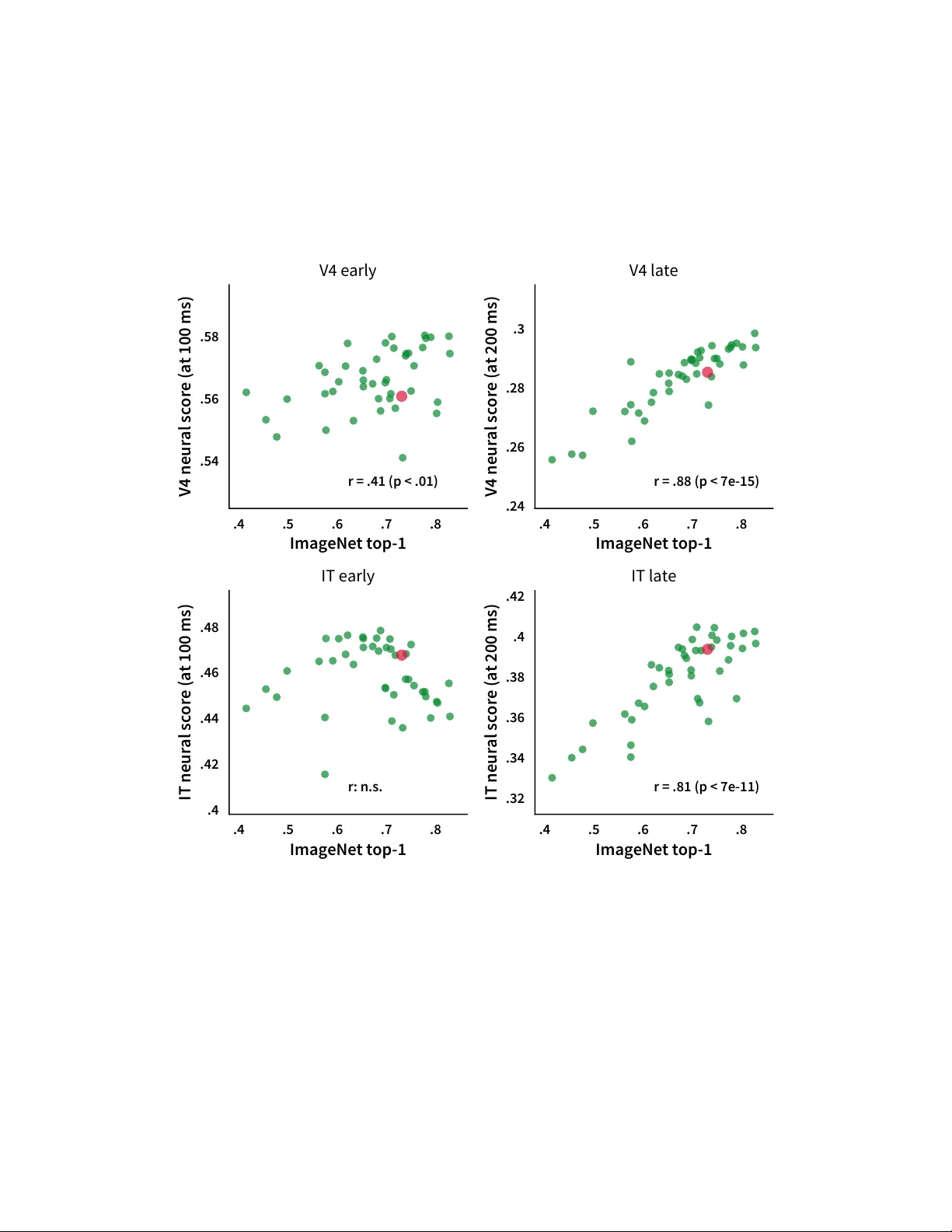
Deep convolutional artificial neural networks (ANNs) are the leading class of candidate models of the mechanisms of visual processing in the primate ventral stream. While initially inspired by brain anatomy, over the past years, these ANNs have evolv…
Authors: Jonas Kubilius, Martin Schrimpf, Kohitij Kar
Brain-Like Object Recognition with High-P erf orming Shallo w Recurrent ANNs Jonas K ubilius *,1,2 , Martin Schrimpf *,1,3,4 , Kohitij Kar 1,3,4 , Rishi Rajalingham 1 , Ha Hong 5 , Najib J. Majaj 6 , Elias B. Issa 7 , Pouya Bashivan 1,3 , Jonathan Pr escott-Roy 1 , Kailyn Schmidt 1 , Aran Nayebi 8 , Daniel Bear 9 , Daniel L. K. Y amins 9,10 , and James J . DiCarlo 1,3,4 1 McGov ern Institute for Brain Research, MIT , Cambridge, MA 02139 2 Brain and Cognition, KU Leuven, Leuv en, Belgium 3 Department of Brain and Cognitiv e Sciences, MIT , Cambridge, MA 02139 4 Center for Brains, Minds and Machines, MIT , Cambridge, MA 02139 5 Bay Labs Inc., San Francisco, CA 94102 6 Center for Neural Science, New Y ork Univ ersity , New Y ork, NY 10003 7 Department of Neuroscience, Zuckerman Mind Brain Behavior Institute, Columbia Univ ersity , Ne w Y ork, NY 10027 8 Neurosciences PhD Program, Stanford Univ ersity , Stanford, CA 94305 9 Department of Psychology , Stanford University , Stanford, CA 94305 10 Department of Computer Science, Stanford Univ ersity , Stanford, CA 94305 * Equal contribution Abstract Deep con volutional artificial neural networks (ANNs) are the leading class of candidate models of the mechanisms of visual processing in the primate ventral stream. While initially inspired by brain anatomy , o ver the past years, these ANNs hav e e volv ed from a simple eight-layer architecture in AlexNet to extremely deep and branching architectures, demonstrating increasingly better object categorization performance, yet bringing into question how brain-lik e they still are. In particular , typical deep models from the machine learning community are often hard to map onto the brain’ s anatomy due to their vast number of layers and missing biologically-important connections, such as recurrence. Here we demonstrate that better anatomical alignment to the brain and high performance on machine learning as well as neuroscience measures do not have to be in contradiction. W e de veloped CORnet-S, a shallo w ANN with four anatomically mapped areas and recurrent connectivity , guided by Brain-Score, a new large-scale composite of neural and behavioral benchmarks for quantifying the functional fidelity of models of the primate ventral visual stream. Despite being significantly shallower than most models, CORnet-S is the top model on Brain-Score and outperforms similarly compact models on ImageNet. Moreov er , our extensi ve analyses of CORnet-S circuitry variants re v eal that recurrence is the main predictive f actor of both Brain- Score and ImageNet top-1 performance. Finally , we report that the temporal ev olution of the CORnet-S "IT" neural population resembles the actual monkey IT population dynamics. T aken together , these results establish CORnet-S, a compact, recurrent ANN, as the current best model of the primate ventral visual stream. 33rd Conference on Neural Information Processing Systems (NeurIPS 2019), V ancouv er , Canada. 0 .2 .4 .6 .8 ImageNet top-1 performance .25 .3 .35 .4 .45 Brain-Score r = .90 .7 .75 .8 .85 ImageNet top-1 performance .37 .38 .39 .4 .41 .42 Brain-Score r: n.s. Figure 1: Synergizing machine learning and neur oscience thr ough Brain-Score (top). By quan- tifying brain-likeness of models, we can compare models of the brain and use insights gained to inform the next generation of models. Green dots represent popular deep neural networks while gray dots correspond to v arious e xemplary small-scale models (BaseNets) that demonstrate the relationship between ImageNet performance and Brain-Score on a wider range of performances (see Section 4.1). CORnet-S is the current best model on Brain-Score. CORnet-S area cir cuitry (bottom left). The model consists of four areas which are pre-mapped to cortical areas V1, V2, V4, and IT in the ventral stream. V1 COR is feed-forward and acts as a pre-processor to reduce the input complexity . V2 COR , V4 COR and IT COR are recurrent (within area). See Section 2.1 for details. 1 Introduction Notorious for their superior performance in object recognition tasks, artificial neural netw orks (ANNs) hav e also witnessed a tremendous success in the neuroscience community as currently the best class of models of the neural mechanisms of visual processing. Surprisingly , after training deep feedforward ANNs to perform the standard ImageNet cate gorization task [ 6 ], intermediate layers in ANNs can partly account for ho w neurons in intermediate layers of the primate visual system will respond to any gi ven image, ev en ones that the model has nev er seen before [ 48 , 50 , 17 , 9 , 4 , 49 ]. Moreover , these networks also partly predict human and non-human primate object recognition performance and object similarity judgments [ 34 , 21 ]. Ha ving strong models of the brain opened up unexpected possibilities of nonin v asi ve brain-machine interfaces where models are used to generate stimuli, optimized to elicit desired responses in primate visual system [2]. How can we push these models to capture brain processing ev en more stringently? Continued architectural optimization on ImageNet alone no longer seems like a viable option. Indeed, more recent and deeper ANNs ha ve not been sho wn to further impro ve on measures of brain-likeness [ 34 ], ev en though their ImageNet performance has v astly increased [ 35 ]. Moreo ver , while the initial limited number of layers could easily be assigned to the different areas of the ventral stream, the link between the handful of ventral stream areas and several hundred layers in ResNet [ 10 ] or complex, branching structures in Inception and N ASNet [ 42 , 27 ] is not ob vious. Finally , high-performing models for object recognition remain feedforward, whereas recent studies established an important functional in v olvement of recurrent processes in object recognition [43, 16]. W e propose that aligning ANNs to neuroanatomy might lead to more compact, interpretable and, most importantly , functionally brain-like ANNs. T o test this, we here demonstrate that a neuroanatomically more aligned ANN, CORnet-S , exhibits an improv ed match to measurements from the ventral stream while maintaining high performance on ImageNet. CORnet-S commits to a shallow recurrent anatomical structure of the ventral visual stream, and thus achie ves a much more compact architecture while retaining a strong ImageNet top-1 performance of 73.1% and setting the new state-of-the-art in predicting neural firing rates and image-by-image human behavior on Brain-Scor e , a nov el large-scale benchmark composed of neural recordings and beha vioral measurements. W e identify that these 2 results are primarily dri ven by recurrent connections, in line with our understanding of how the primate visual system processes visual information [ 43 , 16 ]. In fact, comparing the high le vel ("IT") neural representations between recurrent steps in the model and time-varying primate IT recordings, we find that CORnet-S partly captures these neural response trajectories - the first model to do so on this neural benchmark. 2 CORnet-S: Brain-driven model ar chitectur e W e dev eloped CORnet-S based on the follo wing criteria (based on [20]): (1) Predicti vity , so that it is a mechanistic model of the brain. W e are not only interested in having correct model outputs (behaviors) b ut also internals that match the brain’ s anatomical and functional constraints. W e prefer ANNs because neurons are the units of online information transmission and models without neurons cannot be obviously mapped to neural spiking data [49]. (2) Compactness , i.e. among models with similar scores, we prefer simpler models as they are potentially easier to understand and more efficient to experiment with. Howe ver , there are many ways to define this simplicity . Moti vated by the observation that the feedforw ard path from retinal input to IT is fairly limited in length (e.g., [ 44 ]), for the purposes of this study we use depth as a simple proxy to meeting the biological constraint in artificial neural networks. Here we defined depth as the number of con v olutional and fully connected layers in the longest feedforward path of a model. (3) Recurrence : while core object recognition was originally belie ved to be lar gely feedforw ard because of its fast time scale [ 7 ], it has long been suspected that recurrent connections must be relev ant for some aspects of object perception [ 22 , 1 , 45 ], and recent studies ha ve sho wn their role e ven at short time scales [ 16 , 43 , 36 , 32 , 5 ]. Moreo ver , responses in the visual system ha ve a temporal profile, so models at least should be able to produce responses over time too. 2.1 CORnet-S model specifics CORnet-S (Fig. 1) aims to riv al the best models on Brain-Score by transforming very deep feedforward architectures into a shallow recurrent model. Specifically , CORnet-S draws inspiration from ResNets that are some of the best models on our behavioral benchmark (Fig. 1; [ 34 ]) and can be thought of as unrolled recurrent networks [ 25 ]. Recent studies further demonstrated that weight sharing in ResNets was indeed possible without a significant loss in CIF AR and ImageNet performance [15, 23]. Moreov er , CORnet-S specifically commits to an anatomical mapping to brain areas. While for comparison models we establish this mapping by searching for the layer in the model that best explains responses in a given brain area, ideally such mapping would already be provided by the model, leaving no free parameters. Thus, CORnet-S has four computational areas, conceptualized as analogous to the ventral visual areas V1, V2, V4, and IT , and a linear category decoder that maps from the population of neurons in the model’ s last visual area to its behavioral choices. This simplistic assumption of clearly separate re gions with repeated circuitry w as a first step for us to aim at building as shallow a model as possible, and we are excited about e xploring less constrained mappings (such as just treating everything as a neuron without the distinction into regions) and more diverse circuitry (that might in turn improv e model scores) in the future. Each visual area implements a particular neural circuitry with neurons performing simple canonical computations: con v olution, addition, nonlinearity , response normalization or pooling over a recepti ve field. The circuitry is identical in each of its visual areas (except for V1 COR ), but we vary the total number of neurons in each area. Due to high computational demands, first area V1 COR performs a 7 × 7 con volution with stride 2, 3 × 3 max pooling with stride 2, and a 3 × 3 con volution. Areas V2 COR , V4 COR and IT COR perform tw o 1 × 1 con volutions, a bottleneck-style 3 × 3 con volution with stride 2, expanding the number of features fourfold, and a 1 × 1 con volution. T o implement recurrence, outputs of an area are passed through that area se v eral times. F or instance, after V2 COR processed the input once, that result is passed into V2 COR again and treated as a new input (while the original input is discarded, see "gate" in Fig. 1). V2 COR and IT COR are repeated twice, V4 COR is repeated four times as this results in the most minimal configuration that produced the best model as determined by our scores (see Fig. 4). As in ResNet, each con volution (except the first 1 × 1 ) is followed by batch normalization [ 14 ] and ReLU nonlinearity . Batch normalization was not shared ov er time as suggested by Jastrzebski et al. [15] . There are no across-area bypass or across-area 3 feedback connections in the current definition of CORnet-S and retinal and LGN processing are not explicitly modeled. The decoder part of a model implements a simple linear classifier – a set of weighted linear sums with one sum for each object cate gory . T o reduce the amount of neural responses projecting to this classifier , we first a verage responses ov er the entire recepti ve field per feature map. 2.2 Implementation Details W e used PyT orch 0.4.1 and trained the model using ImageNet 2012 [ 35 ]. Images were preprocessed (1) for training – random crop to 224 × 224 pixels and random flipping left and right; (2) for validation - central crop to 224 × 224 pix els; (3) for Brain-Score – resizing to 224 × 224 pix els. In all cases, this preprocessing was follo wed by normalization by mean subtraction and division by standard de viation of the dataset. W e used a batch size of 256 images and trained on 2 GPUs (NVIDIA Titan X / GeForce 1080T i) for 43 epochs. W e use similar learning rate scheduling to ResNet with more v ariable learning rate updates (primarily in order to train faster): 0.1, di vided by 10 ev ery 20 epochs. For optimization, we use Stochastic Gradient Descent with momentum .9, a cross-entrop y loss between image labels and model predictions (logits). ImageNet-pretrained CORnet-S is av ailable at github .com/dicarlolab/cornet. 2.3 Comparison to other models Liang & Hu [24] introduced a deep recurrent neural network intended for object recognition by adding a variant of a simple recurrent cell to a shallow fi ve-layer con v olutional neural network backbone. Zamir et al. [51] built a more po werful v ersion by employing LSTM cells, and a similar approach was used by [ 39 ] who showed that a simple v ersion of a recurrent net can improve network performance on an MNIST -based task. Liao & Poggio [25] argued that ResNets can be thought of as recurrent neural networks unrolled over time with non-shared weights, and demonstrated the first working version of a folded ResNet, also e xplored by [15]. Ho wev er , all of these networks were only tested on CIF AR-100 at best. As noted by Nayebi et al. [29] , while many netw orks may do well on a simpler task, the y may differentiate once the task becomes sufficiently dif ficult. Moreover , our preliminary testing indicated that non-ImageNet-trained models do not appear to score high on Brain-Score, so e ven for practical purposes we needed models that could be trained on ImageNet. Leroux et al. [23] proposed probably the first recurrent architecture that performed well on ImageNet. In an attempt to explore the recurrent net space in a more principled way , Nayebi et al. [29] performed a large-scale search in the LSTM-based recurrent cell space by allowing the search to find the optimal combination of local and long-range recurrent connections. The best model demonstrated a strong ImageNet performance while being shallo wer than feedforw ard controls. In this w ork, we wanted to go one step further and b uild a maximally compact model that would nonetheless yield top Brain-Score and outperform other recurrent networks on ImageNet. 3 Brain-Score: Comparing models to brain T o obtain quantified scores for brain-likeness, we built Brain-Scor e , a composite benchmark that measures how well models can predict (a) mean neural response of each neural recording site to each and e very tested naturalistic image in non-human primate visual areas V4 and IT (data from [ 28 ]); (b) mean pooled human choices when reporting a target object to each tested naturalistic image (data from [ 34 ]), and (c) when object category is resolved in non-human primate area IT (data from [ 16 ]). T o rank models on an o verall score, we tak e the mean of the beha vioral score, the V4 neural score, the IT neural score, and the neural dynamics score (explained belo w). Brain-Score is open-sourced as a platform to score neural networks on brain data through the Brain-Score.org website for an o vervie w of scores and through github .com/brain-score. 3.1 Neural predicti vity Neural predictivity is used to e valuate ho w well responses to giv en images in a source system (e.g., a deep ANN) predict the responses in a target system (e.g., a single neuron’ s response in visual area IT ; 4 [ 50 ]). As inputs, this metric requires two assemblies of the form stimuli × neuroid where neuroids can either be neural recordings or model activ ations. A total of 2,560 images containing a single object pasted randomly on a natural background were presented centrally to passi vely fixated monk eys for 100 ms and neural responses were obtained from 88 V4 sites and 168 IT sites. F or our analyses, we used normalized time-av eraged neural responses in the 70-170 ms window . For models, we reported the most predictive layer or (for CORnet-S) designated model areas and the best time point. Source neuroids were mapped to each target neuroid linearly using a PLS regression model with 25 components. The mapping procedure was performed for each neuron using 90% of image responses and tested on the remaining 10% in a 10-fold cross-validation strategy with stratification ov er objects. In each run, the weights were fit to map from source neuroids to a target neuroid using training images, and then using these weights predicted responses were obtained for the held-out images. T o speed up this procedure, we first reduced input dimensionality to 1000 components using PCA. W e used the neuroids from V4 and IT separately to compute these fits. The median o ver neurons of the Pearson’ s r between the predicted and actual response constituted the final neural fit score for each visual area. 3.2 Behavioral pr edictivity The purpose of behavioral benchmarks it to compute the similarity between source (e.g., an ANN model) and target (e.g., human or monkey) behavioral responses in any given task [ 34 ]. For core object recognition tasks, primates (both human and monk ey) e xhibit behavioral patterns that dif fer from ground truth labels. Thus, our primary benchmark here is a behavioral response pattern metric, not an ov erall accuracy metric, and higher scores are obtained by ANNs that produce and predict the primate patterns of successes and failures. One consequence of this is that ANNs that achiev e 100% accuracy will not achie ve a perfect beha vioral similarity score. A total of 2,400 images containing a single object pasted randomly on a natural background were presented to 1,472 humans for 100 ms and they were asked to choose from two options which object they saw . For further analyses, we used participants response accuracies of 240 images that had around 60 responses per object-distractor pair (~300,000 unique responses). For ev aluating models, we used model responses to 2,400 images from the layer just prior to 1,000-value cate gory vectors. 2,160 of those images were used to build a 24-way logistic re gression decoder , where each 24-value vector entry is the probability that a giv en object is in the image. This regression was then used to estimate probabilities for the 240 held-out images. Next, both for human model responses, for each image, all normalized object-distractor pair prob- abilities were computed from the 24-way probability vector as follows: p ( truth ) p ( truth )+ p ( choice ) . These probabilities were con verted into a d 0 measure: d 0 = Z ( Hit Rate ) − Z ( F alse Alarms Rate ) , where Z is the estimated z-score of responses, Hit Rate is the accuracy of a gi ven object-distractor pair , and the False Alarms Rate corresponds to ho w often the observers incorrectly reported seeing that target object in images where another object was presented. For instance, if a gi ven image contained a dog and distractor was a bear, the Hit Rate for the dog-bear pair for that image came straight from the 240 × 24 matrix, while in order to obtain the False Alarms Rate, all cells from that matrix that did not hav e dogs in the image b ut had a dog as a distractor were a veraged, and 1 minus that v alue was used as a False Alarm Rate. All d 0 abov e 5 were clipped. This transformation helped to remove bias in responses and also to diminish ceiling effects (since man y primate accuracies were close to 1), but empirically observed benefits of d 0 in this dataset were small; see [ 34 ] for a thorough explanation. The resulting response matrix was further refined by subtracting the mean d 0 across trials of the same object-distractor pair (e.g., for dog-bear trials, their mean was subtracted from each trial). Such normalization exposes v ariance unique to each image and remo ves global trends that may be easier for models to capture. The behavioral predicti vity score was computed as a Pearson’ s r correlation between the actual primate behavioral choices and model’ s predictions. 3.3 Object solution times A total of 1,318 grayscale images, containing images from Section 3.1 and MS COCO [ 26 ], were presented centrally to behaving monke ys for 100 ms and neural responses were obtained from 424 IT sites. Similar to [ 16 ], we fit a linear classifier on 90% of each 10 ms of model acti v ations between 5 70-250 ms and used it to decode object category in each image from the non-overlapping 10% of the data. The linear classifier w as based on a fully-connected layer followed by a softmax, with Xa vier initialization for the weights [ 8 ], l 2 regularized and decaying with 0 . 463 , inputs were z-scored, and fit with a cross-entropy loss, a learning rate of 1 e − 4 ov er 40 epochs with a training batch size of 64, and stopped early if the loss-value went belo w 1 e − 4 . The predictions were con v erted to normalized d 0 scores per image ("I1" in [ 34 ]) and per time bin. By linearly interpolating between these bins, we determined the exact millisecond when the prediction surpassed a threshold value defined by the monkey’ s behavioral output for that image, which we refer to as "object solution times", or OSTs. Images for which either the model or the neural recordings did not produce an OST because the behavioral threshold w as not met were ignored. W e report a Spearman correlation between the model OSTs and the actual monkey OSTs (as computed in [16]). 3.4 Generalization to new datasets Neural: New neur ons, old images W e e v aluated models on an independently collected neural dataset (288 neurons, 2 monkeys, 63 trials per image; [ 16 ]) where new monk eys were presented with a subset of 640 images from the 2,560 images we used for neural predictivity . Neural: New neur ons, new images W e obtained a neural dataset from [ 16 ] for a selection of 1,600 of grayscale MS COCO images [ 26 ]. These images are very dissimilar from the synthetic images we used in other tests, pro viding a strong means to test Brain-Score generalization. The dataset consisted of 288 neurons from 2 monke ys and 45 trials per image. Unlike our previous datasets, this one had a low internal consistenc y between neural responses, presumably due to the electrodes being near their end of life and producing unreasonably high amounts of noise. W e therefore only used the 86 neurons with internal consistency of at least 0.9. Behavioral: New images W e collected a new behavioral dataset, consisting of 200 images (20 objects × 10 images) from Amazon Mechanical T urk users (185,106 trials in total). W e used the same experimental paradigm as in our original behavioral test b ut none of the objects were from the same category as before. CIF AR-100 Follo wing the procedure described in [ 18 ], we tested ho w well these models generalize to CIF AR-100 dataset by only allo wing a linear classifier to be retrained for the 100-way classification task (that is, without doing any fine-tuning). As in [ 18 ], we used a scikit-learn implementation of a multinomial logistic regression using L-BFGS [ 31 ], with the best C parameter found by searching a range from .0005 to .05 in 10 logarithmic steps (40,000 images from CIF AR-100 train set were used for training and the remaining 10,000 for testing; the search range was reduced from [ 18 ] because in our earlier tests we found that all models had their optimal parameters in this range). Accuracies reported on the 10,000 test images. 4 Results 4.1 CORnet-S is the best brain-predicting model so far W e performed a large-scale model comparison using most commonly used neural network fami- lies: AlexNet [ 19 ], VGG [ 38 ], ResNet [ 10 ], Inception [ 40 – 42 ], SqueezeNet [ 13 ], DenseNet [ 12 ], MobileNet [ 11 ], and (P)N ASNet [ 52 , 27 ]. These networks were taken from publicly a vailable check- points: Ale xNet, SqueezeNet, ResNet-{18,34} from PyT orch [ 30 ]; Inception, ResNet-{50,101,152}, (P)N ASNet, MobileNet from T ensorFlo w-Slim [ 37 ]; and Xception, DenseNet, V GG from K eras [ 3 ]. As such, the training procedure is dif ferent between models and our results should be related to those model instantiations and not to architecture families. T o further map out the space of possible architectures, we included a family of models called BaseNets : lightweight AlexNet-like architectures with six con volutional layers and a single fully-connected layer , captured at v arious stages of training. V arious hyperparameters were varied between BaseNets, such as kernel sizes, nonlinearities, learning rate etc. Figure 1 shows ho w models perform on Brain-Score and ImageNet. CORnet-S outperforms other alternativ es by a large margin with the Brain-Score of .471. T op ImageNet models also perform well, with leading models stemming from the DenseNet and ResNet families. Interestingly , models 6 that rank the highest on ImageNet performance are also not the ones scoring high on brain data, suggesting a potential disconnect between ImageNet performance and fidelity to brain mechanisms. For instance, despite its superior performance of 82.9% top-1 accuracy on ImageNet, PNASNet only ranks 13 th on the overall Brain-Score. Models with an ImageNet top-1 performance below 70% sho w a strong correlation with Brain-Score of .90 b ut above 70% ImageNet performance there was no significant correlation ( p . 05 , cf. Figure 1). .53 .55 .57 .6 IT score (original neurons) .5 .52 .54 .56 .58 .6 IT score (new neurons) r = .87 (a) New neural recordings, same images .53 .55 .57 .6 IT score (original neurons) .58 .6 .62 .64 .66 .68 IT score (new neurons) r = .57 (b) New neural recordings, new images .2 .3 .4 Behavioral score (original) .4 .5 .6 Behavioral score (new) r = .85 (c) New behavioral recordings, new images .35 .4 .45 Brain-Score .6 .65 .7 .75 CIFAR-100 transfer r = .64 (d) CIFAR-100 transfer Figure 2: Brain-Score generalization across datasets: (a) to neural recordings in new subjects with the same stimulus set, (b) to neural recordings in new subjects with a very dif ferent stimulus set (MS COCO), (c) to behavioral responses in ne w subjects with ne w object categories, (d) to CIF AR-100. W e further asked if Brain-Score reflects idiosyncracies of the particular datasets that we included in this benchmark or instead, more desirably , provides an ov erall e valuation of ho w brain-lik e models are. T o address this question, we performed four different tests with v arious generalization demands (Fig. 2; CORnet-S w as excluded). First, we compared the scores of models predicting IT neural responses to a set of ne w IT neural recordings [ 16 ] where ne w monkeys were shown the same images as before. W e observed a strong correlation between the tw o sets (Pearson r = . 87 ). When compared on predicting IT responses to a very dif ferent image set (1600 MS COCO images [ 26 ]), model rankings were still strongly correlated (Pearson r = . 57 ). W e also found a strong correlation between model scores on our original beha vioral set and a ne wly obtained set of beha vioral responses to images from 20 new categories that were not used before (200 images total; Pearson r = . 85 ). Finally , we e valuated model feature generalization to CIF AR-100 without fine-tuning (follo wing K ornblith et al. [18] ). Again, we observed a compelling correlation to Brain-Score values (Pearson r = . 64 ). Overall, we expect that adding more benchmarks to Brain-Score will further lead scores to con ver ge. 4.2 CORnet-S is the best on ImageNet and CIF AR-100 among shallow models Due to anatomical constraints imposed by the brain, CORnet-S’ s architecture is much more compact than the majority of deep models in computer vision (Fig. 3 middle). Compared to similar models with a depth less than 50, CORnet-S is shallower yet better than other models on ImageNet top-1 classification accuracy . AlexNet and IamNN are ev en shallower (depth of 8 and 14) but suffer on classification accuracy (57.7% and 69.6% top-1 respectiv ely) – CORnet-S provides a good trade-off between the two with a depth of 15 and top-1 accuracy of 73.1%. Sev eral epochs later in training top-1 accuracy actually climbed to 74.4% but since we are optimizing for the brain, we chose the epoch with maximum Brain-Score. CORnet-S also achie ves the best transfer performance among similarly shallow models (Fig. 3, right), indicating the rob ustness of this model. 4.3 CORnet-S mediates between compactness and high performance thr ough r ecurrence T o determine which elements in the circuitry are critical to CORnet-S, we attempted to alter its block structure and record changes in Brain-Score (Fig. 4). W e only used V4, IT , and behavioral predicti vity in this analysis in order to understand the non-temporal value of CORnet-S structure. W e found that the most important factor was the presence of at least a few steps of recurrence in each block. Ha ving a fairly wide bottleneck (at least 4x expansion) and a skip connection were other important factors. On the other hand, adding more recurrence or ha ving fi ve areas in the model instead of four did not improv e the model or hurt its Brain-Score. Other factors affected mostly ImageNet performance, including using two con volutions instead of three within a block, having more areas in the model and using batch normalization per time step instead of a global group normalization [ 46 ]. The type of gating did not seem to matter . Ho wev er , note that we k ept training with identical hyperparameters 7 10 25 50 100 200 Model Depth (log scale) .34 .36 .38 .4 .42 .44 .46 Brain-Score 10 25 50 100 200 Model Depth (log scale) .4 .5 .6 .7 .8 ImageNet top-1 10 25 50 100 200 Model Depth (log scale) .6 .65 .7 .75 CIFAR-100 transfer Figure 3: Depth v ersus (left) Brain-Score, (middle) ImageNet top-1 performance, and (right) CIF AR-100 transfer performance. Most simple models perform poorly on Brain-Score and Im- ageNet, and generalize less well to CIF AR-100, while the best models are v ery deep. CORnet-S offers the best of both worlds with the best Brain-Score, compelling ImageNet performance, the shallowest architecture we could achiev e to date, and the best transfer performance to CIF AR-100 among shallow models. (Note: dots corresponding to MobileNets were slightly jittered along the x-axis to improv e visibility .) Figure 4: CORnet-S circuitry analysis. Each ro w indicates ho w ImageNet top-1 and Brain-Score change with respect to the baseline model (in bold) when a particular hyperparameter is changed. The OSTs of IT are not included in the Brain-Score here. for all these model v ariants. W e therefore cannot rule out that the reported differences could be minimized if more optimal hyperparameters were found. 4.4 CORnet-S captures neural dynamics in primate IT Feed-forward networks cannot make any dynamic predictions over time, and thus cannot capture a critical property of the primate visual system [ 16 , 43 ]. By introducing recurrence, CORnet-S is capable of producing temporally-varying response trajectories in the same set of neur ons . Recent experimental results [ 16 ] rev eal that the linearly decodable solutions to object recognition are not all produced at the same time in the IT neural population – images that are particularly challenging for deep ANNs take longer to e volv e in IT . This timing provides a strong test for the model: Does it predict image-by-image temporal trajectories in IT neural responses o ver time? W e thus estimated for each image when explicit object cate gory information becomes a vailable in CORnet-S – termed "object solution time" (OST) – and compared it with the same measurements obtained from monkey IT cortex [ 16 ]. Importantly , the model was never trained to predict monkey OSTs. Rather , a linear classifier was trained to decode object category from neural responses and from model’ s responses at each 10 ms window (Section 3.3). OST is defined as the time when this decoding accuracy reaches a threshold defined by monke y behavioral accurac y . W e conv erted the two IT timesteps in CORnet-S to milliseconds by setting t 0 ˆ = 0-150 ms and t 1 ˆ = 150+ ms. W e e valuated ho w well CORnet-S could capture the fine-grained temporal dynamics in primate IT cortex and report a correlation score of .25 ( p < 10 − 6 ; Figure 5). Feed-forward models cannot capture neural dynamics and thus scored 0. 8 5 Discussion Figure 5: CORnet-S captures neural dy- namics. A linear decoder is fit to predict ob- ject category at each 10 ms window of IT re- sponses in model and monkey . W e then tested object solution times (OST) per image, i.e. when d 0 scores of model and monkey surpass the threshold of monkey beha vioral response. r is computed on the ra w data, whereas the plot visualizes binned OSTs. Error bars de- note s.e.m. across images. W e dev eloped a relatively shallow recurrent model CORnet-S that follo ws neuroanatomy more closely than standard machine learning ANNs, and is among the top models on Brain-Score yet remains competi- ti ve on ImageNet and on transfer tests to CIF AR-100. As such, it combines the best of both neuroscience desiderata and machine learning engineering require- ments, demonstrating that models that satisfy both communities can be dev eloped. While we belie ve that CORnet-S is a closer approx- imation to the anatomy of the ventral visual stream than current state-of-the-art deep ANNs because we specifically limit the number of areas and include recurrence, it is still far from complete in many ways. From a neuroscientist’ s point of view , on top of the lack of biologically-plausible learning mechanisms (self-supervised or unsupervised), a better model of the ventral visual pathway would include more anatomical and circuitry-le vel details, such as retina or lateral geniculate nucleus. Similarly , adding a skip connection was not informed by cortical circuitry properties but rather proposed by He et al. [10] as a means to alleviate the degradation problem in very deep architectures. But we note that not just any ar- chitectural choices work. W e ha ve tested hundreds of architectures before finding CORnet-S type of circuitries (Figure 4). A critical component in establishing that models such as CORnet-S are strong candidate models for the brain is Brain-Score, a frame work for quantitati vely comparing any artificial neural network to the brain’ s neural netw ork for visual processing. Even with the relati vely fe w brain benchmarks that we hav e included so far , the frame work already reveals interesting patterns. First, it extends prior work showing that performance correlates with brain similarity . Howe ver , adding recurrence allo ws us to break from this trend and achie ve much better alignment to the brain. Even when the OST measure is not included in Brain-Score, CORnet-S remains one of the top models, indicating its general utility . On the other hand, we also find a potential disconnect between ImageNet performance and Brain-Score with PN ASNet, a state-of-the-art model on ImageNet used in our comparisons, that is not performing well on brain measures, whereas e ven small networks with poor ImageNet performance achiev e reasonable scores. W e further observed that models that score high on Brain-Score also tend to score high on other datasets, supporting the idea that Brain-Score reflects how good a model is ov erall, not just on the four particular neural and behavioral benchmarks that we used. Howe v er , it is possible that the observed lack of correlation is only specific to the way models were trained, as reported recently by Kornblith et al. [18] . For instance, they found that the presence of auxiliary classifiers or label smoothing does not affect ImageNet performance too much but significantly decreases transfer performance, in particular affecting Inception and N ASNet family of models, i.e., the ones that performed worse on Brain-Score than their ImageNet performance would imply . Kornblith et al. [18] reported that retraining these models with optimal settings mark edly improv ed transfer accuracy . Since Brain-Score is also a transfer learning task, we cannot rule out that Brain-Score might change if we retrained the af fected models classes. Thus, we reserv e our claims only about the specific pre-trained models rather than the whole architecture classes. More broadly , we suggest that models of brain processing are a promising opportunity for collab- oration between neuroscience and machine learning. These models ought to be compared through quantified scores on ho w brain-lik e they are, which we here e v aluate with a composite of many neural and behavioral benchmarks in Brain-Score. W ith CORnet-S, we showed that neuroanatomical alignment to the brain in terms of compactness and recurrence can better capture brain processing by predicting neural firing rates, image-by-image behavior , and e ven neural dynamics, while simultane- ously maintaining high ImageNet performance and outperforming similarly compact models. 9 Acknowledgments W e thank Simon K ornblith for helping to conduct transfer tests to CIF AR, and Maryann Rui and Harry Bleyan for the initial prototyping of the CORnet family . This project has receiv ed funding from the European Union’ s Horizon 2020 research and inno vation programme under grant agreement No 705498 (J.K.), US National Eye Institute (R01-EY014970, J.J.D.), Of fice of Nav al Research (MURI-114407, J.J.D), the Simons Foundation (SCGB [325500, 542965], J.J.D; 543061, D.L.K.Y), the James S. McDonnell foundation (220020469, D.L.K.Y .) and the US National Science Foundation (iis-ri1703161, D.L.K.Y .). This work was also supported in part by the Semiconductor Research Corporation (SRC) and D ARP A. The computational resources and services used in this work were provided in part by the VSC (Flemish Supercomputer Center), funded by the Research Foundation - Flanders (FWO) and the Flemish Go vernment – department EWI. References [1] Moshe Bar , Karim S Kassam, A vniel Singh Ghuman, Jasmine Boshyan, Annette M Schmid, Anders M Dale, Matti S Hämäläinen, Ksenija Marinkovic, Daniel L Schacter, Bruce R Rosen, et al. T op-down facilitation of visual recognition. Pr oceedings of the national academy of sciences , 103(2):449–454, 2006. [2] Pouya Bashi van, K ohitij Kar , and James J DiCarlo. Neural population control via deep image synthesis. Science , 364(6439), 2019. [3] François Chollet et al. Keras. https://keras.io , 2015. [4] Radoslaw M Cichy , Aditya Khosla, Dimitrios Pantazis, Antonio T orralba, and Aude Oli v a. Deep neural networks predict hierarchical spatio-temporal cortical dynamics of human visual object recognition. arXiv pr eprint arXiv:1601.02970 , 2016. [5] Alex Clarke, Barry J Devereux, and Lorraine K T yler . Oscillatory dynamics of perceptual to conceptual transformations in the ventral visual pathway . Journal of cognitive neur osc ience , 30(11):1590–1605, 2018. [6] Jia Deng, W ei Dong, Richard Socher , Li-Jia Li, Kai Li, and Li Fei-Fei. ImageNet: A large-scale hierarchical image database. In IEEE Confer ence on Computer V ision and P attern Recognition , pp. 248–255. IEEE, 2009. ISBN 978-1-4244-3992-8. doi: 10.1109/CVPR.2009.5206848. [7] James J DiCarlo, Davide Zoccolan, and Nicole C Rust. How does the brain solv e visual object recognition? Neur on , 73(3):415–434, 2012. [8] Xavier Glorot and Y oshua Bengio. Understanding the difficulty of training deep feedforward neural networks. In International Confer ence on Artificial Intelligence and Statistics (AIST A TS) , pp. 249–256, 2010. [9] Umut Güçlü and Marcel AJ van Gerven. Deep neural networks re veal a gradient in the complexity of neural representations across the ventral stream. J ournal of Neur oscience , 35(27):10005–10014, 2015. [10] Kaiming He, Xiangyu Zhang, Shaoqing Ren, and Jian Sun. Deep residual learning for image recognition. In Pr oceedings of the IEEE confer ence on computer vision and pattern r ecognition , pp. 770–778, 2016. [11] Andrew G. Ho ward, Menglong Zhu, Bo Chen, Dmitry Kalenichenko, W eijun W ang, T obias W eyand, Marco Andreetto, and Hartwig Adam. MobileNets: Efficient Con v olutional Neural Networks for Mobile V ision Applications. arXiv pr eprint arXiv:1704.04861 , 2017. [12] Gao Huang, Zhuang Liu, Laurens V an Der Maaten, and Kilian Q W einber ger . Densely connected con volutional netw orks. In CVPR , 2017. [13] Forrest N. Iandola, Song Han, Matthew W . Moske wicz, Khalid Ashraf, W illiam J. Dally , and Kurt K eutzer . SqueezeNet: AlexNet-le vel accurac y with 50x fe wer parameters and. arXiv pr eprint arXiv:1602.07360 , 2016. [14] Serge y Ioffe and Christian Szegedy . Batch normalization: Accelerating deep network training by reducing internal cov ariate shift. arXiv pr eprint arXiv:1502.03167 , 2015. [15] Stanisław Jastrzebski, Dev ansh Arpit, Nicolas Ballas, V ikas V erma, T ong Che, and Y oshua Bengio. Residual connections encourage iterativ e inference. arXiv pr eprint arXiv:1710.04773 , 2017. 10 [16] K ohitij Kar , Jonas Kubilius, Kailyn Schmidt, Elias B Issa, and James J DiCarlo. Evidence that recurrent cir - cuits are critical to the ventral stream’ s e xecution of core object recognition behavior . Nature neur oscience , pp. 1, 2019. [17] Seyed-Mahdi Khaligh-Raza vi and Nikolaus Kriegesk orte. Deep supervised, but not unsupervised, models may explain it cortical representation. PLoS computational biology , 10(11):e1003915, 2014. [18] Simon K ornblith, Jonathon Shlens, and Quoc V . Le. Do Better ImageNet Models T ransfer Better? arXiv pr eprint arXiv:1805.08974 , 2018. [19] Alex Krizhe vsky , Ilya Sutskev er , and Geoffre y E Hinton. Imagenet classification with deep con volutional neural networks. In Advances in neural information pr ocessing systems , pp. 1097–1105, 2012. [20] Jonas Kubilius. Predict, then simplify . Neur oImage , 180:110 – 111, 2018. [21] Jonas Kubilius, Stef ania Bracci, and Hans P Op de Beeck. Deep neural networks as a computational model for human shape sensitivity . PLoS computational biology , 12(4):e1004896, 2016. [22] V ictor AF Lamme and Pieter R Roelfsema. The distinct modes of vision of fered by feedforward and recurrent processing. T r ends in neur osciences , 23(11):571–579, 2000. [23] Sam Leroux, Pa vlo Molchano v , Pieter Simoens, Bart Dhoedt, Thomas Breuel, and Jan Kautz. Iamnn: Itera- tiv e and adaptiv e mobile neural netw ork for efficient image classification. arXiv pr eprint arXiv:1804.10123 , 2018. [24] Ming Liang and Xiaolin Hu. Recurrent conv olutional neural network for object recognition. In The IEEE Confer ence on Computer V ision and P attern Reco gnition (CVPR) , June 2015. [25] Qianli Liao and T omaso Poggio. Bridging the gaps between residual learning, recurrent neural networks and visual cortex. arXiv pr eprint arXiv:1604.03640 , 2016. [26] Tsung-Y i Lin, Michael Maire, Serge Belongie, James Hays, Pietro Perona, De v a Ramanan, Piotr Dollár , and C Lawrence Zitnick. Microsoft coco: Common objects in context. In European conference on computer vision , pp. 740–755. Springer , 2014. [27] Chenxi Liu, Barret Zoph, Maxim Neumann, Jonathon Shlens, W ei Hua, Li-Jia Li, Li Fei-Fei, Alan Y uille, Jonathan Huang, and Ke vin Murphy . Progressive Neural Architecture Search. arXiv preprint , 2017. [28] Najib J Majaj, Ha Hong, Ethan A Solomon, and James J DiCarlo. Simple learned weighted sums of inferior temporal neuronal firing rates accurately predict human core object recognition performance. J ournal of Neur oscience , 35(39):13402–13418, 2015. [29] Aran Nayebi, Daniel Bear , Jonas Kubilius, Kohitij Kar , Surya Ganguli, Da vid Sussillo, James J DiCarlo, and Daniel LK Y amins. T ask-driv en con volutional recurrent models of the visual system. arXiv preprint arXiv:1807.00053 , 2018. [30] Adam Paszk e, Sam Gross, Soumith Chintala, Gregory Chanan, Edw ard Y ang, Zachary DeV ito, Zeming Lin, Alban Desmaison, Luca Antiga, and Adam Lerer . Automatic dif ferentiation in pytorch. 2017. [31] F . Pedregosa, G. V aroquaux, A. Gramfort, V . Michel, B. Thirion, O. Grisel, M. Blondel, P . Prettenhofer, R. W eiss, V . Dubour g, J. V anderplas, A. Passos, D. Cournapeau, M. Brucher , M. Perrot, and E. Duchesnay . Scikit-learn: Machine learning in Python. Journal of Mac hine Learning Resear ch , 12:2825–2830, 2011. [32] Karim Rajaei, Y alda Mohsenzadeh, Reza Ebrahimpour , and Se yed-Mahdi Khaligh-Razavi. Beyond core object recognition: Recurrent processes account for object recognition under occlusion. bioRxiv , 2018. [33] Rishi Rajalingham, Kailyn Schmidt, and James J DiCarlo. Comparison of object recognition behavior in human and monkey . Journal of Neur oscience , 35(35):12127–12136, 2015. [34] Rishi Rajalingham, Elias B Issa, Pouya Bashiv an, Kohitij Kar, Kailyn Schmidt, and James J DiCarlo. Large-scale, high-resolution comparison of the core visual object recognition beha vior of humans, monkeys, and state-of-the-art deep artificial neural networks. J ournal of Neur oscience , pp. 7255–7269, 2018. [35] Olga Russako vsky , Jia Deng, Hao Su, Jonathan Krause, Sanjeev Satheesh, Sean Ma, Zhiheng Huang, Andrej Karpathy , Aditya Khosla, Michael Bernstein, Alexander C. Berg, and Li Fei-Fei. ImageNet Lar ge Scale V isual Recognition Challenge. International Journal of Computer V ision (IJCV) , 115(3):211–252, 2015. [36] Martin Schrimpf. Brain-inspired recurrent neural algorithms for advanced object recognition. Master’ s thesis, T echnical University Munich, LMU Munich, Uni versity of Augsb urg, 2017. 11 [37] N. Silberman and S. Guadarrama. T ensorflo w-slim image classification model library . https://github. com/tensorflow/models/tree/master/research/slim , 2016. [38] Karen Simonyan and Andrew Zisserman. V ery deep conv olutional networks for large-scale image recogni- tion. arXiv pr eprint arXiv:1409.1556 , 2014. [39] Courtney J Spoerer , Patrick McClure, and Nik olaus Kriegesk orte. Recurrent con volutional neural networks: a better model of biological object recognition. F r ontier s in psychology , 8:1551, 2017. [40] Christian Szegedy , W ei Liu, Y angqing Jia, Pierre Sermanet, Scott Reed, Dragomir Anguelov , Dumitru Erhan, V incent V anhoucke, and Andrew Rabino vich. Going deeper with con volutions. In Proceedings of the IEEE Computer Society Confer ence on Computer V ision and P attern Recognition (CVPR) , sep 2015. ISBN 9781467369640. doi: 10.1109/CVPR.2015.7298594. [41] Christian Szegedy , V incent V anhouck e, Sergey Iof fe, Jonathon Shlens, and Zbignie w W ojna. Rethinking the Inception Architecture for Computer V ision. arXiv pr eprint , 2015. [42] Christian Szegedy , Sergey Iof fe, V incent V anhoucke, and Alexander A Alemi. Inception-v4, inception- resnet and the impact of residual connections on learning. In AAAI , volume 4, pp. 12, 2017. [43] Hanlin T ang, Martin Schrimpf, William Lotter , Charlotte Moerman, Ana Paredes, J.O. Josue Orte ga Caro, W alter Hardesty , Da vid Cox, and Gabriel Kreiman. Recurrent computations for visual pattern completion. Pr oceedings of the National Academy of Sciences (PN AS) , 115(35):8835–8840, 2018. [44] Martin J T ovée. Neuronal processing: How fast is the speed of thought? Current Biology , 4(12):1125–1127, 1994. [45] Johan W agemans, James H Elder , Michael Kubovy , Stephen E Palmer , Mary A Peterson, Manish Singh, and Rüdiger von der He ydt. A century of gestalt psychology in visual perception: I. perceptual grouping and figure–ground organization. Psyc hological b ulletin , 138(6):1172, 2012. [46] Y uxin W u and Kaiming He. Group normalization. arXiv pr eprint arXiv:1803.08494 , 2018. [47] Saining Xie, Ross Girshick, Piotr Dollár, Zhuo wen T u, and Kaiming He. Aggregated residual transfor- mations for deep neural netw orks. In Computer V ision and P attern Reco gnition (CVPR), 2017 IEEE Confer ence on , pp. 5987–5995. IEEE, 2017. [48] Daniel L Y amins, Ha Hong, Charles Cadieu, and James J DiCarlo. Hierarchical modular optimization of con volutional networks achie ves representations similar to macaque it and human v entral stream. In Advances in neural information pr ocessing systems , pp. 3093–3101, 2013. [49] Daniel LK Y amins and James J DiCarlo. Using goal-driven deep learning models to understand sensory cortex. Natur e neur oscience , 19(3):356, 2016. [50] Daniel LK Y amins, Ha Hong, Charles F Cadieu, Ethan A Solomon, Darren Seibert, and James J DiCarlo. Performance-optimized hierarchical models predict neural responses in higher visual cortex. Pr oceedings of the National Academy of Sciences , 111(23):8619–8624, 2014. [51] Amir R Zamir , T e-Lin W u, Lin Sun, William B Shen, Bertram E Shi, Jitendra Malik, and Silvio Sav arese. Feedback networks. In Computer V ision and P attern Reco gnition (CVPR), 2017 IEEE Conference on , pp. 1808–1817. IEEE, 2017. [52] Barret Zoph, V ijay V asudevan, Jonathon Shlens, and Quoc V . Le. Learning Transferable Architectures for Scalable Image Recognition. arXiv pr eprint , 2017. 12 A Numerical Brain-Scores T able 1: Brain-Scores and indi vidual performances for state-of-the-art models Model Brain-Score V4 IT OST Behavior CORnet-S .471 .65 .6 .25 .382 DenseNet-169 .412 .663 .606 0 .378 ResNet-101 v2 .407 .653 .585 0 .389 DenseNet-201 .406 .655 .601 0 .368 DenseNet-121 .406 .657 .597 0 .369 ResNet-152 v2 .406 .658 .589 0 .377 ResNet-50 v2 .405 .653 .589 0 .377 Xception .399 .671 .565 0 .361 Inception v2 .399 .646 .593 0 .357 Inception v1 .399 .649 .583 0 .362 ResNet-18 .398 .645 .583 0 .364 N ASnet Mobile .398 .65 .598 0 .342 PN ASnet Large .396 .644 .59 0 .351 Inception ResNet v2 .396 .639 .593 0 .352 N ASnet Large .395 .65 .591 0 .339 Best MobileNet .395 .613 .59 0 .377 VGG-19 .394 .672 .566 0 .338 Inception V4 .393 .628 .575 0 .371 Inception V3 .392 .646 .587 0 .335 ResNet-34 .392 .629 .559 0 .378 VGG-16 .391 .669 .572 0 .321 Best BaseNet .378 .663 .594 0 .256 AlexNet .366 .631 .589 0 .245 SqueezeNet v1.1 .351 .652 .553 0 .201 SqueezeNet v1.0 .341 .641 .542 0 .18 13 B Brain-Score benchmark details B.1 Brain-Score benchmark T o e valuate how well a model is doing o verall, we computed the global Brain-Score as a composite of neural V4 predictivity score, neural IT predicti vity score, object solution times in IT , and behavioral I2n predicti vity score (each of these scores was computed as described in main te xt). The Brain-Score presented here is the mean of the four scores. This approach of taking the mean does not normalize by different scales of the scores so it may be penalizing scores with low variance. Ho wev er , the alternativ e approach of ranking models on each benchmark separately and then taking the mean rank would impose the strong assumption that for any two models with (even insignificantly) different scores, their ranks are also different. W e thus chose to take the mean score to preserve the distance in values. B.2 Neural recordings The neural dataset currently used in both neural benchmarks included in this version of Brain-Score is comprised of neural responses to 2,560 naturalistic stimuli in 88 V4 neurons and 168 IT neurons, collected by [ 28 ]. The image set consists of 2,560 grayscale images in eight object categories (animals, boats, cars, chairs, faces, fruits, planes, tables). Each category contains eight unique objects (for instance, the “face” category has eight unique faces). The image set was generated by pasting a 3D object model on a naturalist background. In each image, the position, pose, and size of an object was randomly selected in order to create a challenging object recognition task both for primates and machines. A circular mask was applied to each image (see [28] for details on image generation). T wo macaque monke ys were implanted three arrays each, with one array placed in area V4 and the other two placed on the posterior-anterior axis of IT cortex. The monkeys passi vely observed a series of images (100 ms image duration with 100 ms of gap between each image) that each subtended approximately 8 deg visual angle. T o obtain a stable estimate of the neural responses to each image, each each image was re-tested about 50 times (re-tests were randomly interleav ed with other images). In the benchmarks used here, we used an average neural firing rate (normalized to a blank gray image response) in the windo w between 70 ms and 170 ms after image onset where the majority of object category-rele v ant information is contained [28]. B.3 Behavioral r ecordings The behavioral data used in the current round of benchmarks was obtained by [ 33 ] and [ 34 ]. Here we used only the human behavioral data, b ut the human and non-human primate behavioral patterns are very similar to each other [ 33 , 34 ]. The image set used in this data collection was generated in a similar way as the images for V4 and IT using 24 object categories, and human responses were collected on Amazon Mechanical T urk. (Other details are explained in the main text.) 14 C Depth From a neuroscience point of view , simpler models can be better mapped to cortex and be better analyzed and understood with regard to the brain. Simpler models can also be better made sense of sense in terms of what components constitute a strong model by reducing models to their most essential elements. One possibility was to use the total number of parameters (weights). Howe v er , it did not seem to map well to simplicity in neuroscience terms. F or instance, a single con v olutional layer with many filter maps could have man y parameters yet it seems much simpler than a multilayer branching structure, like the Inception block [42], that may ha ve less parameters o verall. Moreov er , our models are always tested on independent data sampled from different distrib utions than the train data. Thus, after training a model, all these parameters were fixed for the purposes of brain benchmarks, and the only free parameters are the ones introduced by the linear decoder that is trained on top of the frozen model’ s parameters (see abo ve for decoder details). W e also considered computing the total number of con volutional and fully-connected layers, but some models, like Inception, perform some con volutions in parallel, while others, like ResNeXt [ 47 ], group multiple conv olutions into a single computation. W e thus decided to use the "longest path" definition as described in the main text. D Predictors of neural scor es W e compared model scores on neural (V4, IT) recordings with the scores on behavioral recordings to see if e.g. a behavioral benchmark alone would already be suf ficient or if the entire set of benchmarks is necessary . W e found that there was a correlation to behavior ( . 65 for V4 and . 87 or IT) which is strong enough to connect neurons to behavior but not suf ficient for beha vior alone to explain the entire neural population, warranting a composite set of benchmarks. Moreov er , we tested if the number of features in model layers might predict the neural scores. Even though we PCA all features to 1,000 components, higher dimensionality might result in better scores. Follo wing Figure 6, we found that neural scores are not consistently correlated with the number of features across neural benchmarks: for V4, ha ving more than 1000 features helps a little ( r = . 46 , p < . 05 ) but for IT , there was no significant correlation at any number of features. 1000 2000 3000 4000 Number of features .6 .62 .64 .66 .68 V4 neural score 1000 2000 3000 4000 Number of features .52 .54 .56 .58 .6 IT neural score Figure 6: Neural Scores do not depend on number of featur es. W e plot the number of features in models’ highest-scoring layers against their neural (V4 and IT) scores. The number of neurons does not appear to be a predictor of better brain-likeness. 15 E Early and late neural predictions Focusing on the temporal aspect of our neural data, we divided spike rates into an early time bin ranging from 90-110 ms and a late time bin from 190-210 ms. W e found that this early-late division highlighted functional model difference more prominently than the mean temporal prediction in [ 29 ]. For instance, Figure 7 shows ho w IT is predicted well by strong ImageNet models at a late stage, but not at early stages. CORnet-S does well on both of these predictions. .4 .5 .6 .7 .8 ImageNet top-1 .54 .56 .58 V4 neural score (at 100 ms) r = .41 (p < .01) V4 early .4 .5 .6 .7 .8 ImageNet top-1 .24 .26 .28 .3 V4 neural score (at 200 ms) r = .88 (p < 7e-15) V4 late .4 .5 .6 .7 .8 ImageNet top-1 .4 .42 .44 .46 .48 IT neural score (at 100 ms) r: n.s. IT early .4 .5 .6 .7 .8 ImageNet top-1 .32 .34 .36 .38 .4 .42 IT neural score (at 200 ms) r = .81 (p < 7e-11) IT late Figure 7: Prediction correlations on early and late spike rates. W e compare ImageNet perfor - mance against pearson correlation of predicted spike rates with neural data binned into early (90-110 ms) and late (190-210 ms). Model mappings are performed separately per bin, layers are chosen based on 70-170 ms scores. Notice ho w better ImageNet models are better at predicting late IT responses, but not early ones. 16 F CORnet-S search 0 .1 .2 .3 .4 .5 .6 .7 ImageNet top-1 0 .05 .1 .15 .2 .25 .3 .35 .4 Behavioral score r = .89 Figure 8: ImageNet top-1 performance vs. beha vioral benchmark on various CORnets. W e manually tried many dif ferent configurations of CORnet circuitry . The figure is showing how behavioral benchmark of Brain-Score is related to ImageNet top-1 performance in 106 CORnet configurations. Each dot corresponds to a particular CORnet at a particular point during training. The correlation between ImageNet top-1 performance and CORnet is rob ust but there is also high variance in this relationship. In particular , notice ho w some models achie ve close to 75% ImageNet performance but sho w only a mediocre behavioral score. Thus, optimizing solely for ImageNet is not guaranteed at all to lead to a good alignment to brain data. 17
Original Paper
Loading high-quality paper...
Comments & Academic Discussion
Loading comments...
Leave a Comment