Correlation Priors for Reinforcement Learning

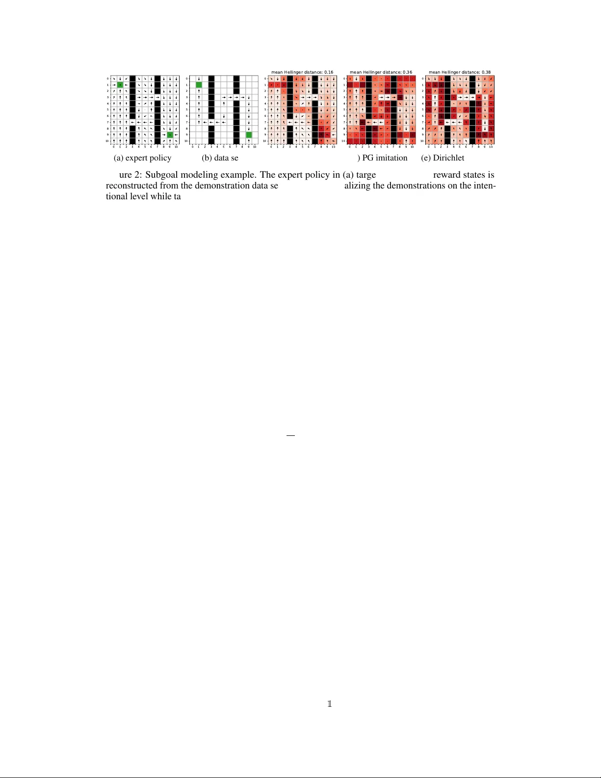
Corr elation Priors f or Reinf or cement Lear ning Bastian Alt ∗ Adrian Šoši ´ c ∗ Heinz Koeppl Department of Electrical Engineering and Information T echnology T echnische Univ ersität Darmstadt {bastian.alt, adrian.sosic, heinz.koeppl}@bcs.tu-darmstadt.de Abstract Many decision-making problems naturally e xhibit pronounced structures inherited from the characteristics of the underlying en vironment. In a Markov decision pro- cess model, for example, two distinct states can ha ve inherently related semantics or encode resembling physical state configurations. This often implies locally cor- related transition dynamics among the states. In order to complete a certain task in such en vironments, the operating agent usually needs to execute a series of tempo- rally and spatially correlated actions. Though there exists a v ariety of approaches to capture these correlations in continuous state-action domains, a principled solution for discrete en vironments is missing. In this work, we present a Bayesian learn- ing framew ork based on Pólya-Gamma augmentation that enables an analogous reasoning in such cases. W e demonstrate the frame work on a number of common decision-making related problems, such as imitation learning, subgoal extraction, system identification and Bayesian reinforcement learning. By e xplicitly modeling the underlying correlation structures of these problems, the proposed approach yields superior predicti ve performance compared to correlation-agnostic models, ev en when trained on data sets that are an order of magnitude smaller in size. 1 Introduction Correlations arise naturally in many aspects of decision-making. The reason for this phenomenon is that decision-making problems often e xhibit pronounced structur es , which substantially influence the strategies of an agent. Examples of correlations are ev en found in stateless decision-making problems, such as multi-armed bandits, where prominent patterns in the rew ard mechanisms of different arms can translate into correlated action choices of the operating agent [ 7 , 9 ]. Howe ver , these statistical relationships become more pronounced in the case of contextual bandits, where effecti ve decision-making strategies not only e xhibit temporal correlation but also tak e into account the state context at each time point, introducing a second source of correlation [12]. In more general decision-making models, such as Markov decision processes (MDPs), the agent can directly affect the state of the en vironment through its action choices. The effects caused by these actions often share common patterns between different states of the process, e.g., because the states hav e inherently related semantics or encode similar physical state configurations of the underlying system. Examples of this general principle are omnipresent in all disciplines and range from robotics, where similar actuator outputs result in similar kinematic responses for similar states of the robot’ s joints, to networking applications, where the servicing of a particular queue affects the surrounding network state (Section 4.3.3). The common consequence is that the structures of the en vironment are usually reflected in the decisions of the operating agent, who needs to ex ecute a series of temporally and spatially correlated actions in order to complete a certain task. This is particularly true when two or more agents interact with each other in the same environment and need coordinate their beha vior [ 2 ]. ∗ The first two authors contrib uted equally to this work. 33rd Conference on Neural Information Processing Systems (NeurIPS 2019), V ancouver , Canada. Focusing on rational beha vior , correlations can manifest themselves e ven in unstructured domains, though at a higher level of abstraction of the decision-making process. This is because rationality itself implies the existence of an underlying objectiv e optimized by the agent that represents the agent’ s intentions and incenti vizes to choose one action o ver another . T ypically , these goals persist at least for a short period of time, causing dependencies between consecutiv e action choices (Section 4.2). In this paper , we propose a learning framew ork that offers a direct way to model such correlations in finite decision-making problems, i.e., in volving systems with discrete state and action spaces. A key feature of our frame work is that it allows to capture correlations at an y le vel of the process, i.e., in the system environment, at the intentional lev el, or directly at the le vel of the ex ecuted actions. W e encode the underlying structure in a hierarchical Bayesian model, for which we deri ve a tractable variational inference method based on Pólya-Gamma augmentation that allows a fully probabilistic treatment of the learning problem. Results on common benchmark problems and a queueing network simulation demonstrate the advantages of the frame work. The accompanying code is publicly av ailable via Git. 1 Related W ork Modeling correlations in decision-making is a common theme in reinforcement learning and related fields. Gaussian processes (GPs) offer a flexible tool for this purpose and are widely used in a broad variety of conte xts. Moreov er , mov ement primiti ves [ 18 ] provide an ef fecti ve way to describe temporal relationships in control problems. Howe ver , the natural problem domain of both are continuous state-action en vironments, which lie outside the scope of this work. Inferring correlation structure from count data has been discussed extensiv ely in the context of topic modeling [ 13 , 14 ] and factor analysis [ 29 ]. Recently , a GP classification algorithm with a scalable vari- ational approach based on Pólya-Gamma augmentation was proposed [ 30 ]. Though these approaches are promising, they do not address the problem-specific modeling aspects of decision-making. For agents acting in discrete en vironments, a number of customized solutions e xist that allo w to model specific characteristics of a decision-making problem. A broad class of methods that specifically target temporal correlations rely on hidden Marko v models. Many of these approaches operate on the intentional le vel, modeling the temporal relationships of the different goals follo wed by the agent [ 22 ]. Howe ver , there also exist several approaches to capture spatial dependencies between these goals. For a recent overvie w , see [ 27 ] and the references therein. Dependencies on the action level hav e also been considered in the past but, like most intentional models, existing approaches lar gely focus on the temporal correlations in action sequences (such as probabilistic movement primiti v es [ 18 ]) or they are restricted to the special case of deterministic policies [ 26 ]. A probabilistic frame work to capture correlations between discrete action distributions is described in [25]. When it comes to modeling transition dynamics, most existing approaches rely on GP models [ 4 , 3 ]. In the T explore method of [ 8 ], correlations within the transition dynamics are modeled with the help of a random forest, creating a mixture of decision tree outcomes. Y et, a full Bayesian description in form of an explicit prior distribution is missing in this approach. For behavior acquisition, prior distributions ov er transition dynamics are adv antageous since they can easily be used in Bayesian reinforcement learning algorithms such as BEETLE [ 21 ] or B AMCP [ 6 ]. A particular example of a prior distrib ution ov er transition probabilities is giv en in [ 19 ] in the form of a Dirichlet mixture. Howe ver , the incorporation of prior knowledge expressing a particular correlation structure is difficult in this model. T o the best of our knowledge, there exists no principled method to e xplicitly model correlations in the transition dynamics of discrete en vironments. Also, a univ ersally applicable inference tool for discrete en vironments, comparable to Gaussian processes, has not yet emerged. The goal of our work is to fill this gap by providing a fle xible inference frame work for such cases. 2 Background 2.1 Markov Decision Pr ocesses In this paper , we consider finite Markov decision processes (MDPs) of the form ( S , A , T , R ) , where S = { 1 , . . . , S } is a finite state space containing S distinct states, A = { 1 , . . . , A } is an action space 1 https://git.rwth- aachen.de/bcs/correlation_priors_for_rl 2 comprising A actions for each state, T : S × S × A → [0 , 1] is the state transition model specifying the probability distrib ution ov er next states for each current state and action, and R : S × A → R is a rew ard function. For further details, see [28]. 2.2 Inference in MDPs In decision-making with discrete state and action spaces, we are often faced with integer -v alued quantities modeled as draws from multinomial distributions, x c ∼ Mult( x c | N c , p c ) , N c ∈ N , p c ∈ ∆ K , where K denotes the number of cate gories, c ∈ C index es some finite co v ariate space with cardinality C , and p c parametrizes the distribution at a gi ven co variate v alue c . Herein, x c can either represent actual count data observed during an experiment or describe some latent variable of our model. For example, when modeling the policy of an agent in an MDP , x c may represent the vector of action counts observed at a particular state, in which case C = S , K = A , and N c is the total number of times we observe the agent choosing an action at state c . Similarly , when modeling state transition probabilities, x c could be the vector counting outgoing transitions from some state s for a giv en action a (in which case C = S × A ) or , when modeling the agent’ s intentions, x c could describe the number of times the agent follows a particular goal, which itself might be unobservable (Section 4.2). When facing the in verse problem of inferring the probability vectors { p c } from the count data { x c } , a computationally straightforward approach is to model the probability vectors using independent Dirichlet distributions for all cov ariate v alues, i.e., p c ∼ Dir( p c | α c ) ∀ c ∈ C , where α c ∈ R K > 0 is a local concentration parameter for covariate v alue c . Howe ver , the resulting model is agnostic to the rich correlation structure present in most MDPs (Section 1) and thus ignores much of the prior information we hav e about the underlying decision-making problem. A more natural approach would be to model the probability vectors { p c } jointly using common prior model, in order to capture their dependency structure. Unfortunately , this renders exact posterior inference intractable, since the resulting prior distributions are no longer conjugate to the multinomial lik elihood. Recently , a method for approximate inference in dependent multinomial models has been developed to account for the inherent correlation of the probability vectors [ 14 ]. T o this end, the following prior model was introduced, p c = Π SB ( ψ c · ) , ψ · k ∼ N ( ψ · k | µ k , Σ ) , k = 1 , . . . , K − 1 . (1) Herein, Π SB ( ζ ) = [Π (1) SB ( ζ ) , . . . , Π ( K ) SB ( ζ )] > is the logistic stic k-br eaking transformation , where Π ( k ) SB ( ζ ) = σ ( ζ k ) Y j and κ k = [ κ 1 k , . . . , κ C k ] > . A detailed deriv ation of the these results and the resulting ELBO is provided in Section A . The v ariational approximation can be optimized through coordinate-wise ascent by cycling through the parameters and their moments. The corresponding distribution o ver probability v ectors { p c } is defined implicitly through the deterministic relationship in Eq. (1). 4 Hyper -Parameter Optimization For hyper -parameter learning, we employ a v ariational expectation-maximization approach [ 15 ] to optimize the ELBO after each update of the variational parameters. Assuming a cov ariance matrix Σ θ parametrized by a vector θ = [ θ 1 , . . . , θ J ] > , the ELBO can be written as L ( q ) = − K − 1 2 | Σ θ | + 1 2 K − 1 X k =1 log | V k | − 1 2 K − 1 X k =1 tr ( Σ − 1 θ V k ) − 1 2 K − 1 X k =1 ( µ k − λ k ) > Σ − 1 θ ( µ k − λ k ) + C ( K − 1) + K − 1 X k =1 C X c =1 log  b ck x ck  − K − 1 X k =1 C X c =1 b ck log 2 + K − 1 X k =1 λ > k κ k − K − 1 X k =1 C X c =1 b ck log  cosh w ck 2  . A detailed deri v ation of this expression can be found in Section A.2. The corresponding gradients w .r .t. the hyper-parameters calculate to ∂ L ∂ µ k = Σ θ − 1 ( µ k − λ k ) , ∂ L ∂ θ j = − 1 2 K − 1 X k =1  tr ( Σ − 1 θ ∂ Σ θ ∂ θ j ) − tr ( Σ − 1 θ ∂ Σ θ ∂ θ j Σ − 1 θ V k ) − ( µ k − λ k ) > Σ − 1 θ ∂ Σ θ ∂ θ j Σ − 1 θ ( µ k − λ k )  , which admits a closed-form solution for the optimal mean parameters, giv en by µ k = λ k . For the optimization of the co variance parameters θ , we can resort to a numerical scheme using the abov e gradient expression; ho we ver , this requires a full in version of the covariance matrix in each update step. As it turns out, a closed-form expression can be found for the special case where θ is a scale parameter, i.e., Σ θ = θ ˜ Σ , for some fixed ˜ Σ . The optimal parameter value can then be determined as θ = 1 K C K − 1 X k =1 tr  ˜ Σ − 1  V k + ( µ k − λ k )( µ k − λ k ) >   . The closed-form solution a v oids repeated matrix in versions since ˜ Σ − 1 , being independent of all hyper- parameters and variational parameters, can be e v aluated at the start of the optimization procedure. The full deriv ation of the gradients and the closed-form expression is provided in Section B. For the e xperiments in the following section, we consider a squared exponential co v ariance function of the form ( Σ θ ) cc 0 = θ exp  − d ( c,c 0 ) 2 l 2  , with a cov ariate distance measure d : C × C → R ≥ 0 and a length scale l ∈ R ≥ 0 adapted to the specific modeling scenario. Y et, we note that for model selection purposes multiple cov ariance functions can be easily compared against each other based on the resulting values of the ELBO [ 15 ]. Also, a combination of functions can be employed, provided that the resulting cov ariance matrix is positi ve semi-definite (see co v ariance kernels of GPs [23]). 4 Experiments T o demonstrate the versatility of our inference framew ork, we test it on a number of modeling scenar- ios that commonly occur in decision-making contexts. Due to space limitations, we restrict ourselves to imitation learning, subgoal modeling, system identification, and Bayesian reinforcement learning. Howe ver , we would like to point out that the same modeling principles can be applied in many other situations, e.g., for beha vior coordination among agents [ 2 ] or kno wledge transfer between related tasks [ 11 ], to name just tw o examples. A more comprehensiv e e v aluation study is left for future work. 4.1 Imitation Learning First, we illustrate our framework on an imitation learning example, where we aspire to reconstruct the policy of an agent (in this conte xt called the expert ) from observed beha vior . For the reconstruction, 5 0 1 2 3 4 5 6 7 8 9 0 1 2 3 4 5 6 7 8 9 (a) expert polic y 0 1 2 3 4 5 6 7 8 9 0 1 2 3 4 5 6 7 8 9 (b) Dirichlet estimate 0 1 2 3 4 5 6 7 8 9 0 1 2 3 4 5 6 7 8 9 (c) PG estimate 0.0 0.2 0.4 0.6 0.8 1.0 Hellinger value loss Dirichlet PG (d) normalized ev aluation metrics Figure 1: Imitation learning example. The expert policy in (a) is reconstructed using the posterior mean estimates of (b) an independent Dirichlet policy model and (c) a correlated PG model, based on action data observed at the states marked in gray . The PG joint estimate of the local policies yields a significantly improv ed reconstruction, as sho wn by the resulting Hellinger distance to the expert policy and the corresponding v alue loss [27] in (d). we suppose to have access to a demonstration data set D = { ( s d , a d ) ∈ S × A} D d =1 containing D state-action pairs, where each action has been generated through the e xpert policy , i.e., a d ∼ π ( a | s d ) . Assuming a discrete state and action space, the policy can be represented as a stochastic matrix Π = [ π 1 , . . . , π S ] , whose i th column π i ∈ ∆ A represents the local action distribution of the e xpert at state i in form of a vector . Our goal is to estimate this matrix from the demonstrations D . By constructing the count matrix ( X ) ij = P D d =1 1 ( s d = i ∧ a d = j ) , the inference problem can be directly mapped to our PG model, which allows to jointly estimate the coupled quantities { π i } through their latent representation Ψ by approximating the posterior distribution p ( Ψ | X ) in Eq. (2). In this case, the cov ariate set C is described by the state space S . T o demonstrate the advantages of this joint inference approach over a correlation-agnostic estimation method, we compare our framework to the independent Dirichlet model described in Section 2.2. Both reconstruction methods are e valuated on a classical grid world scenario comprising S = 100 states and A = 4 actions. Each action triggers a noisy transition in one of the four cardinal directions such that the pattern of the resulting next-state distrib ution resembles a discretized Gaussian distribution centered around the targeted adjacent state. Rew ards are distributed randomly in the en vironment. The expert follows a near-optimal stochastic policy , choosing actions from a softmax distribution obtained from the Q-values of the current state. An example scenario is sho wn in Fig. 1a, where the the displayed arro ws are obtained by weighting the four unit-length vectors associated with the action set A according to their local action probabilities. The rew ard locations are highlighted in green. Fig. 1b shows the reconstruction of the policy obtained through the independent Dirichlet model. Since no dependencies between the local action distrib utions are considered in this approach, a posterior esti- mate can only be obtained for states where demonstration data is available, highlighted by the gray col- oring of the background. For all remaining states, the mean estimate predicts a uniform action choice for the e xpert beha vior since no action is preferred by the symmetry of the Dirichlet prior , resulting in an effecti ve arrow length of zero. By contrast, the PG model (Fig. 1c) is able to generalize the expert behavior to unobserv ed regions of the state space, resulting in significantly improv ed reconstruction of the polic y (Fig. 1d). T o capture the underling correlations, we used the Euclidean distance between the grid positions as cov ariate distance measure d and set l to the maximum occurring distance value. 4.2 Subgoal Modeling In many situations, modeling the actions of an agent is not of primary interest or proves to be difficult, e.g., because a more comprehensiv e understanding of the agent’ s behavior is desired (see in verse reinforcement learning [ 16 ] and preference elicitation [ 24 ]) or because the policy is of complex form due to intricate system dynamics. A typical example is robot object manipulation, where contact-rich dynamics can make it difficult for a controller trained from a small number of demonstrations to appropriately generalize the e xpert behavior [ 31 ]. A simplistic example illustrating this problem is depicted in Fig. 2a, where the agent behavior is heavily affected by the geometry of the en vironment and the action profiles at tw o wall-separated states dif fer drastically . Similarly to Section 4.1, we aspire to reconstruct the shown beha vior from a demonstration data set of the form D = { ( s d , a d ) ∈ S × A} D d =1 , depicted in Fig. 2b. This time, ho wev er , we follow a conceptually 6 0 1 2 3 4 5 6 7 8 9 10 0 1 2 3 4 5 6 7 8 9 10 (a) expert polic y 0 1 2 3 4 5 6 7 8 9 10 0 1 2 3 4 5 6 7 8 9 10 (b) data set 0 1 2 3 4 5 6 7 8 9 10 0 1 2 3 4 5 6 7 8 9 10 mean Hellinger distance: 0.16 (c) PG subgoal 0 1 2 3 4 5 6 7 8 9 10 0 1 2 3 4 5 6 7 8 9 10 mean Hellinger distance: 0.36 (d) PG imitation 0 1 2 3 4 5 6 7 8 9 10 0 1 2 3 4 5 6 7 8 9 10 mean Hellinger distance: 0.38 (e) Dirichlet subgoal Figure 2: Subgoal modeling example. The expert polic y in (a) targeting the green re ward states is reconstructed from the demonstration data set in (b). By generalizing the demonstrations on the inten- tional le v el while taking into account the geometry of the problem, the PG subgoal model in (c) yields a significantly improved reconstruction compared to the corresponding action-based model in (d) and the uncorrelated subgoal model in (e). Red color encodes the Hellinger distance to the expert policy . dif ferent line of reasoning and assume that each state s ∈ S has an associated subgoal g s that the agent is targeting at that state. Thus, action a d is considered as being drawn from some goal-dependent action distribution p ( a d | s d , g s d ) . For our e xample, we adopt the normalized softmax action model described in [ 27 ]. Spatial relationships between the agent’ s decisions are taken into account with the help of our PG framework, by coupling the probability vectors that go vern the underlying subgoal selection process, i.e., g s ∼ Cat( p s ) , where p s is described through the stick-breaking construction in Eq. (1). Accordingly , the underlying cov ariate space of the PG model is C = S . W ith the additional le vel of hierarchy introduced, the count data X to train our model is not directly av ailable since the subgoals { g s } S s =1 are not observable. For demonstration purposes, instead of deri ving the full v ariational update for the extended model, we follow a simpler strategy that lev erages the existing inference frame work within a Gibbs sampling procedure, switching between v ariational updates and drawing posterior samples of the latent subgoal v ariables. More precisely , we iterate be- tween 1) computing the v ariational approximation in Eq. (3) for a gi ven set of subgoals { g s } S s =1 , treat- ing each subgoal as single observation count, i.e., x s = OneHot( g s ) ∼ Mult( x s | N s = 1 , p s ) and 2) updating the latent assignments based on the induced goal distributions, i.e., g s ∼ Cat(Π SB ( ψ s · )) . Fig. 2c shows the policy model obtained by a veraging the predicti ve action distrib utions of M = 100 drawn subgoal configurations, i.e., ˆ π ( a | s ) = 1 M P M m =1 p ( a | s, g h m i s ) , where g h m i s denotes the m th Gibbs sample of the subgoal assignment at state s . The obtained reconstruction is visibly better than the one produced by the corresponding imitation learning model in Fig. 2d, which interpolates the behavior on the action le vel and thus fails to navig ate the agent around the walls. While the Dirichlet- based subgoal model (Fig. 2e) can generally account for the walls through the use of the underlying softmax action model, it cannot propagate the goal information to un visited states. For the considered uninformati ve prior distribution over subgoal locations, this has the consequence that actions assigned to such states hav e the tendency to transport the agent to the center of the en vironment, as this is the dominating mov e obtained when blindly av eraging ov er all possible goal locations. 4.3 System Identification & Bayesian Reinf orcement Lear ning Having focused our attention on learning a model of an observed policy , we now enter the realm of Bayesian reinforcement learning (BRL) and optimize a beha vioral model to the particular dynamics of a gi ven en vironment. For this purpose, we slightly modify our grid world from Section 4.1 by placing a target re ward of +1 in one corner and repositioning the agent to the opposite corner whenev er the target state is reached (compare “Grid10” domain in [ 6 ]). For the experiment, we assume that the agent is aware of the tar get re ward b ut does not kno w the transition dynamics of the en vironment. 4.3.1 System Identification For the be ginning, we ignore the re ward mechanism altogether and focus on learning the transition dynamics of the en vironment. T o this end, we let the agent perform a random walk on the grid, choosing actions uniformly at random and observing the resulting state transitions. The recorded state-action sequence ( s 1 , a 1 , s 2 , a 2 , . . . , a T − 1 , s T ) is summarized in the form of count matrices [ X (1) , . . . , X ( A ) ] , where the element ( X ( a ) ) ij = P T t =1 1 ( a t = a ∧ s t = i ∧ s t +1 = j ) represents 7 Dir ( α = 10 − 3 ) sampling Dir ( α = 10 − 3 ) mean Dir ( α = 1) sampling Dir ( α = 1) mean PG sampling PG mean 0 2000 4000 6000 8000 10000 n um b er of transitions 0 . 2 0 . 4 0 . 6 0 . 8 Hellinger distance (a) transition model error 0 500 1000 1500 2000 n um b er of transitions 0 . 00 0 . 25 0 . 50 0 . 75 1 . 00 normalized v alue (b) model-based BRL Figure 3: Bayesian reinforcement learning results. (a) Estimation error of the transition dynamics ov er the number of observed transitions. Sho wn are the Hellinger distances to the true next-state distribution and the standard deviation of the estimation error , both av eraged over all states and actions of the MDP . (b) Expected returns of the learned policies (normalized by the optimal return) when replanning with the estimated transition dynamics after ev ery fiftieth state transition. the number of observed transitions from state i to j for action a . Analogously to the previous two experiments, we estimate the transition dynamics of the environment from these matrices using an independent Dirichlet prior model and our PG framew ork, where we employ a separate model for each transition count matrix. The resulting estimation accuracy is described by the graphs in Fig. 3a, which sho w the distance between the ground truth dynamics of the en vironment and those predicted by the models, av eraged o ver all states and actions. As expected, our PG model significantly outperforms the naiv e Dirichlet approach. 4.3.2 Bayesian Reinf orcement Lear ning Next, we consider the problem of combined model-learning and decision-making by exploiting the experience gathered from previous system interactions to optimize future behavior . Bayesian reinforcement learning of fers a natural playground for this task as it intrinsically balances the importance of information gathering and instantaneous reward maximization, av oiding the exploration- exploitation dilemma encountered in classical reinforcement learning schemes [5]. T o determine the optimal trade-off between these two competing objectiv es computationally , we follow the principle of posterior sampling for r einfor cement learning (PSRL) [ 17 ], where future actions are planned using a probabilistic model of the en vironment’ s transition dynamics. Herein, we consider two v ariants: (1) In the first variant, we compute the optimal Q-values for a fixed number of posterior samples representing instantiations of the transition model and choose the policy that yields the highest expected return on average. (2) In the second variant, we select the greedy policy dictated by the posterior mean of the transition dynamics. In both cases, the obtained policy is followed for a fixed number of transitions before ne w observations are taken into account for updating the posterior distribution. Fig. 3b shows the expected returns of the so-obtained policies o ver the entire e xecution period for the three prior models ev aluated in Fig. 3a and both PSRL variants. The graphs rev eal that the PG approach requires significantly fe wer transitions to learn an effecti v e decision-making strate gy . 4.3.3 Queueing Network Modeling As a final experiment, we e v aluate our model on a network scheduling problem, depicted in Fig. 4a. The considered two-server network consists of two queues with buf fer lengths B 1 = B 2 = 10 . The state of the system is determined by the number of packets in each queue, summarized by the queueing vector b = [ b 1 , b 2 ] , where b i denotes the number of packets in queue i . The underlying system state space is S = { 0 , . . . , B 1 } × { 0 , . . . , B 2 } with size S = ( B 1 + 1)( B 2 + 1) . For our experiment, we consider a system with batch arriv als and batch servicing. The task for the agent is to schedule the traffic flo w of the network under the condition that only one of the queues can be processed at a time. Accordingly , the actions are encoded as a = 1 for serving queue 1 and a = 2 for serving queue 2. The number of packets arriving at queue 1 is modeled as 8 | {z } B 2 q 3 b 2 z}|{ | {z } B 1 q 1 q 2 b 1 z }| { (a) queueing network 0 20 40 60 80 episo de − 10 − 9 − 8 − 7 − 6 v alue PG Dir α = 1 Dir α = 10 − 3 (b) comparison of learned policies Figure 4: BRL for batch queueing. (a) Considered two-server queueing network. (b) Expected returns ov er the number of learning episodes, each consisting of twenty state transitions. q 1 ∼ P ois( q 1 | ϑ 1 ) with mean rate ϑ 1 = 1 . The packets are transferred to buf fer 1 and subsequently processed in batches of random size q 2 ∼ Pois( q 2 | ϑ 2 ) , provided that the agent selects queue 1. Therefore, ϑ 2 = β 1 1 ( a = 1) , where we consider an av erage batch size of β 1 = 3 . Processed packets are transferred to the second queue, where they wait to be processed further in batches of size q 3 ∼ Pois( q 3 | ϑ 3 ) , with ϑ 3 = β 2 1 ( a = 2) and an average batch size of β 2 = 2 . The resulting transition to the new queueing state b 0 after one processing step can be compactly written as b 0 = [( b 1 + q 1 − q 2 ) B 1 0 , ( b 2 + q 2 − q 3 ) B 2 0 ] , where the truncation operation ( · ) B 0 = max(0 , min( B , · )) accounts for the nonnegati vity and finiteness of the buf fers. The reward function, which is kno wn to the agent, computes the ne gati ve sum of the queue lengths R ( b ) = − ( b 1 + b 2 ) . Despite the simplistic architecture of the network, finding an optimal policy for this problem is challenging since determining the state transition matrices requires nontrivial calculations in volving concatenations of Poisson distributions. More importantly , when applied in a real-world conte xt, the arri v al and processing rates of the network are typically unkno wn so that planning-based methods cannot be applied. Fig. 4b sho ws the ev aluation of PSRL on the network. As in the pre vious experiment, we use a separate PG model for each action and compute the cov ariance matrix Σ θ based on the normalized Euclidean distances between the queueing states of the system. This encodes our prior kno wledge that the queue lengths obtained after servicing two independent copies of the network tend to be similar if their pre vious b uf fer states were similar . Our agent follows a greedy strategy w .r .t. the posterior mean of the estimated model. The policy is e valuated after each polic y update by performing one thousand steps from all possible queueing states of the system. As the graphs reveal, the PG approach significantly outperforms its correlation agnostic counterpart, requiring fe wer interactions with the system while yielding better scheduling strategies by generalizing the networks dynamics o ver queueing states. 5 Conclusion W ith the proposed variational PG model, we ha ve presented a self-contained learning framew ork for flexible use in many common decision-making conte xts. The framework allo ws an intuitiv e consider - ation of prior knowledge about the beha vior of an agent and the structures of its en vironment, which can significantly boost the predictiv e performance of the resulting models by leveraging correlations and reoccurring patterns in the decision-making process. A k ey feature is the adjustment of the model regularization through automatic calibration of its hyper-parameters to the specific decision-making scenario at hand, which provides a built-in solution to infer the ef fecti ve range of correlations from the data. W e hav e e valuated the framework on various benchmark tasks including a realistic queueing problem, which in a real-world situation admits no planning-based solution due to unkno wn system parameters. In all presented scenarios, our frame work consistently outperformed the naive baseline methods, which neglect the rich statistical relationships to be unra veled in the estimation problems. Acknowledgments This work has been funded by the German Research F oundation (DFG) as part of the projects B4 and C3 within the Collaborativ e Research Center (CRC) 1053 – MAKI. 9 References [1] D. M. Blei, A. Kucukelbir , and J. D. McAuliffe. V ariational inference: A revie w for statisticians. Journal of the American Statistical Association , 112(518):859–877, 2017. [2] G. Chalkiadakis and C. Boutilier . Coordination in multiagent reinforcement learning: A Bayesian approach. In International Joint Confer ence on Autonomous Agents and Multiag ent Systems , pages 709–716. A CM, 2003. [3] M. Deisenroth and C. E. Rasmussen. Pilco: A model-based and data-efficient approach to polic y search. In International Confer ence on Machine Learning , pages 465–472, 2011. [4] Y . Engel, S. Mannor, and R. Meir . Bayes meets Bellman: The Gaussian process approach to temporal difference learning. In International Conference on Machine Learning , pages 154–161, 2003. [5] M. Ghav amzadeh, S. Mannor, J. Pineau, A. T amar, et al. Bayesian reinforcement learning: A survey . F oundations and T r ends in Machine Learning , 8(5-6):359–483, 2015. [6] A. Guez, D. Silver , and P . Dayan. Efficient Bayes-adaptiv e reinforcement learning using sample-based search. In Advances in Neural Information Pr ocessing Systems , pages 1025–1033, 2012. [7] S. Gupta, G. Joshi, and O. Y a ˘ gan. Correlated multi-armed bandits with a latent random source. arXiv:1808.05904 , 2018. [8] T . Hester and P . Stone. T explore: real-time sample-efficient reinforcement learning for robots. Machine learning , 90(3):385–429, 2013. [9] M. Hof fman, B. Shahriari, and N. Freitas. On correlation and budget constraints in model-based bandit optimization with application to automatic machine learning. In Artificial Intelligence and Statistics , pages 365–374, 2014. [10] H. Ishwaran and L. F . James. Gibbs sampling methods for stick-breaking priors. Journal of the American Statistical Association , 96(453):161–173, 2001. [11] T . W . Killian, S. Daulton, G. K onidaris, and F . Doshi-V elez. Robust and ef ficient transfer learning with hidden parameter Markov decision processes. In Advances in Neural Information Processing Systems , pages 6250–6261, 2017. [12] A. Krause and C. S. Ong. Conte xtual Gaussian process bandit optimization. In Advances in Neural Information Pr ocessing Systems , pages 2447–2455, 2011. [13] J. D. Lafferty and D. M. Blei. Correlated topic models. In Advances in Neural Information Pr ocessing Systems , pages 147–154, 2006. [14] S. Linderman, M. Johnson, and R. P . Adams. Dependent multinomial models made easy: Stick-breaking with the Pólya-Gamma augmentation. In Advances in Neural Information Processing Systems , pages 3456–3464, 2015. [15] K. P . Murphy . Machine learning: a pr obabilistic perspective . MIT Press, 2012. [16] A. Y . Ng and S. J. Russell. Algorithms for in verse reinforcement learning. In International Conference on Machine Learning , pages 663–670, 2000. [17] I. Osband, D. Russo, and B. V an Roy . (More) efficient reinforcement learning via posterior sampling. In Advances in Neural Information Pr ocessing Systems , pages 3003–3011, 2013. [18] A. Paraschos, C. Daniel, J. R. Peters, and G. Neumann. Probabilistic movement primiti ves. In Advances in Neural Information Pr ocessing Systems , pages 2616–2624, 2013. [19] M. Pavlov and P . Poupart. T owards global reinforcement learning. In NIPS W orkshop on Model Uncertainty and Risk in Reinfor cement Learning , 2008. [20] N. G. Polson, J. G. Scott, and J. Windle. Bayesian inference for logistic models using Pólya-Gamma latent variables. Journal of the American Statistical Association , 108(504):1339–1349, 2013. [21] P . Poupart, N. Vlassis, J. Hoey , and K. Regan. An analytic solution to discrete Bayesian reinforcement learning. In International Conference on Mac hine Learning , pages 697–704. A CM, 2006. [22] P . Ranchod, B. Rosman, and G. Konidaris. Nonparametric Bayesian reward segmentation for skill discov ery using in verse reinforcement learning. In IEEE/RSJ International Conference on Intelligent Robots and Systems , pages 471–477, 2015. 10 [23] C. E. Rasmussen and C. K. I. W illiams. Gaussian Pr ocesses for machine learning . MIT Press, 2005. [24] C. A. Rothkopf and C. Dimitrakakis. Preference elicitation and in verse reinforcement learning. In Joint Eur opean Confer ence on Machine Learning and Knowledg e Discovery in Databases , pages 34–48, 2011. [25] A. Šoši ´ c, A. M. Zoubir , and H. K oeppl. A Bayesian approach to policy recognition and state representation learning. IEEE T ransactions on P attern Analysis and Machine Intelligence , 40(6):1295–1308, 2017. [26] A. Šoši ´ c, A. M. Zoubir, and H. Koeppl. Policy recognition via expectation maximization. In IEEE International Confer ence on Acoustics, Speech and Signal Pr ocessing , pages 4801–4805, 2016. [27] A. Šoši ´ c, E. Rueckert, J. Peters, A. M. Zoubir, and H. K oeppl. In verse reinforcement learning via nonparametric spatio-temporal subgoal modeling. Journal of Machine Learning Resear ch , 19(69):1–45, 2018. [28] R. S. Sutton and A. G. Barto. Reinforcement learning: An introduction . MIT Press, 2018. [29] M. K. T itsias. The infinite Gamma-Poisson feature model. In Advances in Neural Information Pr ocessing Systems , pages 1513–1520, 2008. [30] F . W enzel, T . Galy-Fajou, C. Donner , M. Kloft, and M. Opper . Efficient Gaussian process classification using Pòlya-Gamma data augmentation. In AAAI Conference on Artificial Intelligence , v olume 33, pages 5417–5424, 2019. [31] Y . Zhu, Z. W ang, J. Merel, A. Rusu, T . Erez, S. Cabi, S. Tun yasuvunakool, J. Kramár , R. Hadsell, N. de Fre- itas, et al. Reinforcement and imitation learning for div erse visuomotor skills. , 2018. 11 Corr elation Priors f or Reinf orcement Lear ning — Supplementary Material — Bastian Alt Adrian Šoši ´ c Heinz Koeppl Department of Electrical Engineering and Information T echnology T echnische Univ ersität Darmstadt {bastian.alt, adrian.sosic, heinz.koeppl}@bcs.tu-darmstadt.de A Optimizing the Evidence Lower Bound (ELBO) In this section, we provide the detailed calculation for optimizing the ELBO of the presented model. First, we deri ve the optimal v ariational distrib utions and their parameters in Section A.1. Then, we deriv e the ELBO as function of the v ariational parameters in Section A.2. The ELBO for the proposed model with PG augmentation scheme is L ( q ) = E [log p ( Ψ , Ω , X )] − E [log q ( Ψ , Ω )] . (5) The joint distribution of the model is gi ven by p ( Ψ , Ω , X ) = K − 1 Y k =1 N ( ψ · k | µ k , Σ ) × C Y c =1  b ck x ck  2 − b ck exp( κ ck ψ ck ) exp( − ω ck ψ 2 ck / 2) PG( ω ck | b ck , 0) . (6) For the deri v ation, we assume a factorized approximation with q ( Ψ , Ω ) = K − 1 Y k =1 q ( ψ · k ) C Y c =1 q ( ω ck ) . (7) A.1 Parameteric F orms of the V ariational Distributions Calculating the V ariational Distribution q ( ψ · k ) First, we calculate the optimal forms of the variational distributions q ( ψ · k ) , k = 1 , . . . , K − 1 . Collecting all terms in Eq. (5) that depend on ψ · k giv es L ( q ) = L ( q ( ψ · k )) + L const . Due to the factorization in Eq. (7) together with Eq. (6), we ha ve L ( q ( ψ · k )) = E [log N ( ψ · k | µ k , Σ )] + C X c =1 E [ ψ ck ] κ ck − C X c =1 E [ ω ck ψ 2 ck / 2] − E [log q ( ψ · k )] . The optimal distribution can be calculated by introducing the Lagrangian L ( q ( ψ · k ) , ν ) = E [log N ( ψ · k | µ k , Σ )] + C X c =1 E [ ψ ck ] κ ck − C X c =1 E [ ω ck ψ 2 ck / 2] − E [log q ( ψ · k )] + ν  Z q ( ψ · k ) d ψ · k − 1  , 12 which ensures that q ( ψ · k ) is a proper density , using ν as a Lagrange multiplier to enforce the normalization constraint. The Euler Lagrange equation and optimality condition are δ L δ q = 0 , ∂ L ∂ ν = 0 . (8) The functional deriv ative of the Lagrangian yields δ L δ q = log N ( ψ · k | µ k , Σ ) + C X c =1 ψ ck κ ck − C X c =1 E [ ω ck ] ψ 2 ck / 2 − log q ( ψ · k ) − 1 + ν. By solving the Euler Lagrange equation for q ( ψ · k ) , we obtain q ( ψ · k ) = exp ν − 1 + log N ( ψ · k | µ k , Σ ) + C X c =1 ψ ck κ ck − C X c =1 E [ ω ck ] ψ 2 ck / 2 ! . The optimality condition (normalization constraint) in Eq. (8) yields q ( ψ · k ) ∝ N ( ψ · k | µ k , Σ ) exp − 1 2 C X c =1 E [ ω ck ] ψ 2 ck + C X c =1 ψ ck κ ck ! ∝ N ( ψ · k | µ k , Σ ) C Y c =1 N ( κ ck E [ ω ck ] | ψ ck , 1 / E [ ω ck ]) = N ( ψ · k | µ k , Σ ) N (diag ( E [ ω k ]) − 1 κ k | ψ · k , diag ( E [ ω k ]) − 1 ) . Therefore, the optimal distribution q ( ψ · k ) can be identified as a Gaussian by completing the square q ( ψ · k ) = N ( ψ · k | λ k , V k ) , (9) with the variational parameters V k = ( Σ − 1 + diag ( E [ ω k ])) − 1 , λ k = V k ( κ k + Σ − 1 µ k ) . (10) Calculating the V ariational Distribution q ( ω ck ) The distrib ution for q ( ω ck ) is calculated in a similar fashion. The ELBO in Eq. (5) in terms dependent on ω ck can be written as L ( q ( ω ck )) = L ( q ( ω ck )) + L const , with L ( q ( ω ck )) = − E [ ω ck ] E [ ψ 2 ck ] / 2 + E [log PG( ω ck | b ck , 0)] − E [log q ( ω ck )] . The Lagrangian for the distribution q ( ω ck ) is L ( q ( ω ck ) , ν ) = − E [ ω ck ] E [ ψ 2 ck ] / 2 + E [log PG( ω ck | b ck , 0)] − E [log q ( ω ck )] + ν  Z q ( ω ck ) dω ck − 1  The functional deriv ative of the Lagrangian yields δ L δ q = − ω ck E [ ψ 2 ck ] / 2 + log PG( ω ck | b ck , 0) − log q ( ω ck ) − 1 + ν. Solving the Euler Lagrange equation δ L δ q = 0 for q ( ω ck ) , we find q ( ω ck ) = exp  ν − 1 + log PG( ω ck | b ck , 0) − ω ck E [ ψ 2 ck ] / 2  . The normalization constraint is used to identify q ( ω ck ) ∝ PG( ω ck | b ck , 0) exp  − ω ck E [ ψ 2 ck ] / 2  . By exploiting the e xponential tilting property of the PG distribution, that is, PG( ζ | u, v ) ∝ exp( − v 2 2 ζ ) PG( ζ | u, 0) , we obtain q ( ω ck ) = PG( ω ck | b ck , w ck ) , (11) with the variational parameter w ck = p E [ ψ 2 ck ] . 13 A.2 The ELBO for the Optimal Distrib utions The ELBO L ( q ) = E [log p ( Ψ , Ω , X )] − E [log q ( Ψ , Ω )] in terms of the previously deri ved optimal distributions calculates to E [log p ( Ψ , Ω , X )] = K − 1 X k =1 E [log N ( ψ · k | µ k , Σ )] + K − 1 X k =1 C X c =1 log  b ck x ck  − K − 1 X k =1 C X c =1 b ck log 2 + K − 1 X k =1 λ > k κ k + K − 1 X k =1 C X c =1 E [log PG( ω ck | b ck , w ck )] − K − 1 X k =1 C X c =1 b ck log  cosh w ck 2  , E [log q ( Ψ , Ω )] = K − 1 X k =1 E [log N ( ψ · k | λ k , V k )] + K − 1 X k =1 C X c =1 E [log PG( ω ck | b ck , w ck )] . Canceling out the terms E [log PG( ω ck | b ck , w ck )] and re writing the prior and v ariational terms as Kullback-Leibler (KL) di ver gence, we obtain L ( q ) = − K − 1 X k =1 KL ( N ( ψ · k | λ k , V k ) k N ( ψ · k | µ k , Σ )) + K − 1 X k =1 C X c =1 log  b ck x ck  − K − 1 X k =1 C X c =1 b ck log 2 + K − 1 X k =1 λ > k κ k − K − 1 X k =1 C X c =1 b ck log  cosh w ck 2  . Finally , by computing the KL di ver gence, the ELBO can be expressed in terms of the variational parameters as L ( q ) = − K − 1 2 | Σ | + 1 2 K − 1 X k =1 log | V k | − 1 2 K − 1 X k =1 tr ( Σ − 1 V k ) − 1 2 K − 1 X k =1 ( µ k − λ k ) > Σ − 1 ( µ k − λ k ) + C ( K − 1) + K − 1 X k =1 C X c =1 log  b ck x ck  − K − 1 X k =1 C X c =1 b ck log 2 + K − 1 X k =1 λ > k κ k − K − 1 X k =1 C X c =1 b ck log  cosh w ck 2  . (12) B Hyper -P arameter Optimization In this section, we provide a deri vation for the optimization of the hyper -parameters. By maximizing the ELBO L ( q ) w .r .t. the parameters µ k and the parameterized covariance matrix Σ θ , we obtain equations for the variational e xpectation maximization algorithm. The ELBO as a function of the mean µ k and cov ariance Σ θ can be written as L ( Σ θ , µ k ) = − K − 1 2 | Σ θ | − 1 2 K − 1 X k =1 tr ( Σ − 1 θ V k ) − 1 2 K − 1 X k =1 ( µ k − λ k ) > Σ − 1 θ ( µ k − λ k ) + L const . (13) 14 B.1 Derivation of the Optimal V alue f or the Mean µ k W e calculate the gradient of Eq. (13) as ∂ L ∂ µ k = Σ − 1 θ ( µ k − λ k ) . Setting the gradient to zero, we obtain µ k = λ k . (14) B.2 Derivation of the Optimal Hyper -Parameters of Σ θ W e calculate the gradient of Eq. (13) as ∂ L ∂ θ j = − K − 1 2 tr ( Σ − 1 θ ∂ Σ θ ∂ θ j ) + 1 2 K − 1 X k =1 tr ( Σ − 1 θ ∂ Σ θ ∂ θ j Σ − 1 θ V k ) + 1 2 K − 1 X k =1 ( µ k − λ k ) > Σ − 1 θ ∂ Σ θ ∂ θ j Σ − 1 θ ( µ k − λ k ) . (15) When considering the special case of a scaled co v ariance matrix Σ θ = θ ˜ Σ , we can find the optimizing hyper-parameter θ in closed form. Note that ∂ Σ θ ∂ θ = ˜ Σ and Σ − 1 θ = 1 θ ˜ Σ − 1 . Therefore, the gradient computes to ∂ L ∂ θ = − K 2 θ tr ( I ) + 1 2 θ 2 K − 1 X k =1 tr ( ˜ Σ − 1 V k ) + 1 2 θ 2 K − 1 X k =1 ( µ k − λ k ) > ˜ Σ − 1 ( µ k − λ k ) . Setting the deriv ative to zero and solving for θ , we obtain the closed-form expression θ = 1 K S K − 1 X k =1 tr  ˜ Σ − 1  V k + ( µ k − λ k )( µ k − λ k ) >   . (16) 15