Seeing What a GAN Cannot Generate

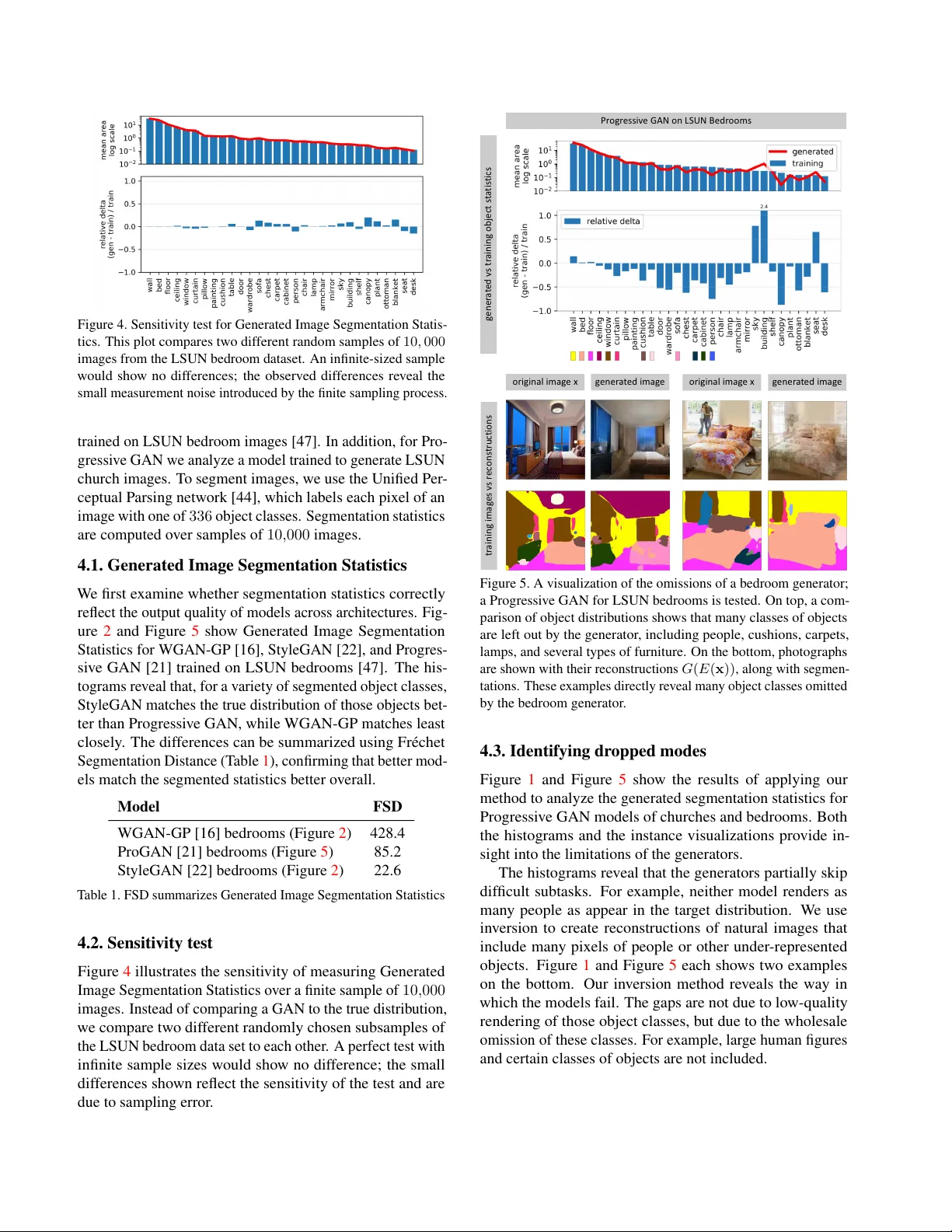
Seeing What a GAN Cannot Generate David Bau 1,2 , Jun-Y an Zhu 1 , Jonas W ulf f 1 , W illiam Peebles 1 Hendrik Strobelt 2 , Bolei Zhou 3 , Antonio T orralba 1,2 1 MIT CSAIL, 2 MIT -IBM W atson AI Lab, 3 The Chinese Uni versity of Hong K ong Abstract Despite the success of Generative Adver sarial Networks (GANs), mode collapse r emains a serious issue during GAN training . T o date, little work has focused on understand- ing and quantifying which modes have been dr opped by a model. In this work, we visualize mode collapse at both the distribution le vel and the instance level. F irst, we deploy a semantic se gmentation network to compar e the distribution of segmented objects in the gener ated images with the tar- get distrib ution in the tr aining set. Differ ences in statistics r eveal object classes that ar e omitted by a GAN. Second, given the identified omitted object classes, we visualize the GAN’ s omissions directly . In particular , we compare specific differ ences between individual photos and their appr oximate in versions by a GAN. T o this end, we relax the pr oblem of in version and solve the tr actable pr oblem of inverting a GAN layer instead of the entir e generator . F inally , we use this framework to analyze several r ecent GANs tr ained on multiple datasets and identify their typical failur e cases. 1. Introduction The remarkable ability of a Generative Adv ersarial Network (GAN) to synthesize realistic images leads us to ask: Ho w can we know what a GAN is unable to generate? Mode- dropping or mode collapse, where a GAN omits portions of the tar get distrib ution, is seen as one of the biggest challenges for GANs [ 14 , 24 ], yet current analysis tools pro vide little insight into this phenomenon in state-of-the-art GANs. Our paper aims to provide detailed insights about dropped modes. Our goal is not to measure GAN quality using a sin- gle number: existing metrics such as Inception scores [ 34 ] and Fr ´ echet Inception Distance [ 17 ] focus on that problem. While those numbers measure how far the generated and target distrib utions are from each other , we instead seek to understand what is different between real and fake images. Existing literature typically answers the latter question by sampling generated outputs, but such samples only visualize what a GAN is capable of doing. W e address the complemen- tary problem: we want to see what a GAN cannot generate. original image reconstru ction original image reconstruction Progress ive GAN on LSUN Chur ches (a) generated vs tr aining obj ect segmentation statisti cs (b) real ima ges vs . recon struction s Figure 1. Seeing what a GAN cannot generate: (a) W e compare the distribution of object segmentations in the training set of LSUN churches [ 47 ] to the distribution in the generated results: objects such as people, cars, and fences are dropped by the generator . (b) W e compare pairs of a real image and its reconstruction in which individual instances of a person and a fence cannot be generated. In each block, we show a real photograph (top-left), a generated re- construction (top-right), and segmentation maps for both (bottom). In particular , we wis h to know: Does a GAN devi ate from the target distribution by ignoring dif ficult images altogether? Or are there specific, semantically meaningful parts and objects that a GAN decides not to learn about? And if so, how can we detect and visualize these missing concepts that a GAN does not generate? Image generation methods are typically tested on images of faces, objects, or scenes. Among these, scenes are an especially fertile test domain as each image can be parsed into clear semantic components by segmenting the scene into objects. Therefore, we propose to directly understand mode dropping by analyzing a scene generator at two levels: the distribution le vel and instance lev el. First, we characterize omissions in the distribution as a whole, using Generated Image Segmentation Statistics : we segment both generated and ground truth images and compare the distrib utions of se gmented object classes. For example, Figure 1 a shows that in a church GAN model, object classes such as people, cars, and fences appear on fe wer pixels of the generated distribution as compared to the training distribution. Second, once omitted object classes are identified, we want to visualize specific examples of failure cases. T o do so, we must find image instances where the GAN should generate an object class but does not. W e find such cases using a new reconstruction method called Layer In version which relaxes reconstruction to a tractable problem. Instead of inv erting the entire GAN, our method inv erts a layer of the generator . Unlike existing methods to in vert a small gen- erator [ 51 , 8 ], our method allo ws us to create reconstructions for complex, state-of-the-art GANs. Deviations between the original image and its reconstruction re veal image features and objects that the generator cannot draw faithfully . W e apply our framework to analyze sev eral recent GANs trained on dif ferent scene datasets. Surprisingly , we find that dropped object classes are not distorted or rendered in a low quality or as noise. Instead, they are simply not rendered at all, as if the object was not part of the scene . For example, in Figure 1 b, we observe that lar ge human figures are skipped entirely , and the parallel lines in a fence are also omitted. Thus a GAN can ignore classes that are too hard, while at the same time producing outputs of high a verage visual quality . Code, data, and additional information are available at ganseeing.csail.mit.edu . 2. Related work Generative Adv ersarial Networks [15] hav e enabled many computer vision and graphics applications such as generation [ 7 , 21 , 22 ], image and video manipulation [ 19 , 20 , 30 , 35 , 39 , 41 , 52 ], object recognition [ 6 , 42 ], and text- to-image translation [ 33 , 45 , 49 ]. One important issue in this emerging topic is ho w to ev aluate and compare different methods [ 40 , 43 ]. For example, many e valuation metrics hav e been proposed to ev aluate unconditional GANs such as Inception score [ 34 ], Fr ´ echet Inception Distance [ 17 ], and W asserstein Sliced Distance [ 21 ]. Though the abov e met- rics can quantify different aspects of model performance, they cannot e xplain what visual content the models fail to synthesize. Our goal here is not to introduce a metric. In- stead, we aim to provide explanations of a common failure case of GANs: mode collapse. Our error diagnosis tools complement existing single-number metrics and can provide additional insights into the model’ s limitations. Network in version. Prior work has found that in ver - sions of GAN generators are useful for photo manipula- tion [ 2 , 8 , 31 , 51 ] and unsupervised feature learning [ 10 , 12 ]. Later work found that DCGAN left-inv erses can be com- puted to high precision [ 25 , 46 ], and that inv ersions of a GAN for glyphs can rev eal specific strokes that the gener - ator is unable to generate [ 9 ]. While pre vious work [ 51 ] has in vestigated inv ersion of 5-layer DCGAN generators, we find that when moving to a 15-layer Progressi ve GAN, high-quality in versions are much more difficult to obtain. In our work, we dev elop a layer-wise in version method that is more ef fective for these large-scale GANs. W e apply a classic layer-wise training approach [ 5 , 18 ] to the problem of training an encoder and further introduce layer-wise image- specific optimization. Our work is also loosely related to in version methods for understanding CNN features and clas- sifiers [ 11 , 27 , 28 , 29 ]. Howe ver , we focus on understanding generativ e models rather than classifiers. Understanding and visualizing networks. Most prior work on network visualization concerns discriminati ve clas- sifiers [ 1 , 3 , 23 , 26 , 37 , 38 , 48 , 50 ]. GANs have been visual- ized by examining the discriminator [32] and the semantics of internal features [ 4 ]. Different from recent work [ 4 ] that aims to understand what a GAN has learned, our work pro- vides a complementary perspective and focuses on what semantic concepts a GAN fails to capture. 3. Method Our goal is to visualize and understand the semantic concepts that a GAN generator cannot generate, in both the entire dis- tribution and in each image instance. W e will proceed in two steps. First, we measure Gener ated Image Se gmentation Statistics by se gmenting both generated and target images and identifying types of objects that a generator omits when compared to the distribution of real images. Second, we visualize ho w the dropped object classes are omitted for indi- vidual images by finding real images that contain the omitted classes and projecting them to their best reconstruction giv en an intermediate layer of the generator . W e call the second step Layer In version . 3.1. Quantifying distribution-le vel mode collapse The systematic errors of a GAN can be analyzed by exploit- ing the hierarchical structure of a scene image. Each scene has a natural decomposition into objects, so we can estimate deviations from the true distrib ution of scenes by estimating deviations of constituent object statistics. For e xample, a WGAN - GP on LSUN Bedrooms StyleGAN on LSUN Bedrooms Figure 2. Using Generated Image Segmentation Statistics to understand the different behavior of the two models trained on LSUN bedrooms [ 47 ]. The histograms re veal that WGAN-GP [ 16 ] (left) deviates from the true distribution much more than StyleGAN [ 22 ] (right), identifying segmentation classes that are generated too little and others that are generated too much. For e xample, WGAN-GP does not generate enough pixels containing beds, curtains, or cushions compared to the true distrib ution of bedroom images, while StyleGAN correctly matches these statistics. StyleGAN is still not perfect, howe ver , and does not generate enough doors, wardrobes, or people. Numbers abov e bars indicate clipped values be yond the range of the chart. GAN that renders bedrooms should also render some amount of curtains. If the curtain statistics depart from what we see in true images, we will kno w we can look at curtains to see a specific flaw in the GAN. T o implement this idea, we segment all the images using the Unified Perceptual Parsing network [ 44 ], which labels each pixel of an image with one of 336 object classes. Over a sample of images, we measure the total area in pix els for each object class and collect mean and cov ariance statistics for all segmented object classes. W e sample these statistics ov er a large set of generated images as well as training set images. W e call the statistics ov er all object se gmentations Generated Imag e Segmentation Statistics . Figure 2 visualizes mean statistics for two netw orks. In each graph, the mean segmentation frequenc y for each gen- erated object class is compared to that seen in the true dis- tribution. Since most classes do not appear on most images, we focus on the most common classes by sorting classes by descending frequency . The comparisons can rev eal many specific dif ferences between recent state-of-the-art models. Both analyzed models are trained on the same image distri- bution (LSUN bedrooms [ 47 ]), but WGAN-GP [ 16 ] departs from the true distribution much more than StyleGAN [22]. It is also possible to summarize statistical dif ferences in segmentation in a single number . T o do this, we define the Fr ´ echet Segmentation Distance (FSD), which is an inter- pretable analog to the popular Fr ´ echet Inception Distance (FID) metric [ 17 ]: FSD ≡ || µ g − µ t || 2 + T r(Σ g + Σ t − 2(Σ g Σ t ) 1 / 2 ) . In our FSD formula, µ t is the mean pixel count for each object class over a sample of training images, and Σ t is the cov ariance of these pixel counts. Similarly , µ g and Σ g reflect segmentation statistics for the generati ve model. In our experiments, we compare statistics between 10 , 000 generated samples and 10 , 000 natural images. Generated Image Segmentation Statistics measure the en- tire distribution: for e xample, they rev eal when a generator omits a particular object class. Howe ver , they do not single out specific images where an object should have been gener- ated but w as not. T o gain further insight, we need a method to visualize omissions of the generator for each image. 3.2. Quantifying instance-lev el mode collapse T o address the above issue, we compare image pairs ( x , x 0 ) , where x is a real image that contains a particular object class dropped by a GAN generator G , and x 0 is a projection onto the space of all images that can be generated by a layer of the GAN model. Defining a tractable inv ersion problem. In the ideal case, we would lik e to find an image that can be per- fectly synthesized by the generator G and stay close to the real image x . Formally , we seek x 0 = G ( z ∗ ) , where z ∗ = arg min z ` ( G ( z ) , x ) and ` is a distance metric in im- age feature space. Unfortunately , as shown in Section 4.4 , previous methods [ 10 , 51 ] fail to solve this full inv ersion problem for recent generators due to the lar ge number of lay- ers in G . Therefore, we instead solve a tractable subproblem of full in version. W e decompose the generator G into layers G = G f ( g n ( · · · (( g 1 ( z )))) , (1) where g 1 , ..., g n are se veral early layers of the generator , and G f groups all the later layers of the G together . Any image that can be generated by G can also be gen- erated by G f . That is, if we denote by range( G ) the generator G encoder E loss reco nst ru cti on G f (r*) targe t x n th layer z 0 r 0 G(z 0 ) targe t x r G f Step 2: initialize z 0 = E( x) r 0 = g n (…(g 1 (z 0 ))) Step 3: optimiz e G f (r ) à x r ≈ r 0 +δ i z 0 generator G encoder E z syn th es ize d G( z) z' loss Step 1 : train encoder E E(G(z)) à z G f G f Figure 3. Overvie w of our layer in version method. First, we train a network E to in vert G ; this is used to obtain an initial guess of the latent z 0 = E ( x ) and its intermediate representation r 0 = g n ( · · · ( g 1 ( z 0 ))) . Then r 0 is used to initialize a search for r ∗ to obtain a reconstruction x 0 = G f ( r ∗ ) close to the target x . set of all images that can be output by G , then we hav e range( G ) ⊂ range( G f ) . That implies, con versely , that any image that cannot be generated by G f cannot be generated by G either . Therefore any omissions we can identify in range( G f ) will also be omissions of range( G ) . Thus for layer in version, we visualize omissions by solv- ing the easier problem of in verting the later layers G f : x 0 = G f ( r ∗ ) , (2) where r ∗ = arg min r ` ( G f ( r ) , x ) . Although we ultimately seek an intermediate represen- tation r , it will be helpful to begin with an estimated z : an initial guess for z helps us regularize our search to fav or v alues of r that are more likely to be generated by a z . There- fore, we solve the in version problem in two steps: First we construct a neural network E that approximately in verts the entire G and computes an estimate z 0 = E ( x ) . Sub- sequently we solve an optimization problem to identify an intermediate representation r ∗ ≈ r 0 = g n ( · · · ( g 1 ( z 0 ))) that generates a reconstructed image G f ( r ∗ ) to closely recov er x . Figure 3 illustrates our layer in version method. Layer -wise network in version. A deep network can be trained more easily by pre-training indi vidual layers on smaller problems [ 18 ]. Therefore, to learn the in verting neural network E , we also proceed layer-wise. For each layer g i ∈ { g 1 , ..., g n , G f } , we train a small network e i to approximately in vert g i . That is, defining r i = g i ( r i − 1 ) , our goal is to learn a network e i that approximates the compu- tation r i − 1 ≈ e i ( r i ) . W e also want the predictions of the network e i to well preserve the output of the layer g i , so we want r i ≈ g i ( e i ( r i )) . W e train e i to minimize both left- and right-in version losses: L L ≡ E z [ || r i − 1 − e ( g i ( r i − 1 )) || 1 ] L R ≡ E z [ || r i − g i ( e ( r i )) || 1 ] e i = arg min e L L + λ R L R , (3) T o focus on training near the manifold of representations produced by the generator, we sample z and then use the layers g i to compute samples of r i − 1 and r i , so r i − 1 = g i − 1 ( · · · g 1 ( z ) · · · ) . Here || · || 1 denotes an L1 loss, and we set λ R = 0 . 01 to emphasize the reconstruction of r i − 1 . Once all the layers are inv erted, we can compose an in- version network for all of G : E ∗ = e 1 ( e 2 ( · · · ( e n ( e f ( x ))))) . (4) The results can be further improved by jointly fine-tuning this composed network E ∗ to inv ert G as a whole. W e denote this fine-tuned result as E . Layer -wise image optimization. As described at the be- ginning of Section 3.2 , in verting the entire G is dif ficult: G is non-con vex, and optimizations ov er z are quickly trapped in local minima. Therefore, after obtaining a decent initial guess for z , we turn our attention to the more relaxed opti- mization problem of in verting the layers G f ; that is, starting from r 0 = g n ( · · · ( g 1 ( z 0 ))) , we seek an intermediate repre- sentation r ∗ that generates a reconstructed image G f ( r ∗ ) to closely recov er x . T o re gularize our search to fav or r that are close to the representations computed by the early layers of the genera- tor , we search for r that can be computed by making small perturbations of the early layers of the generator: z 0 ≡ E ( x ) r ≡ δ n + g n ( · · · ( δ 2 + g 2 ( δ 1 + g 1 ( z 0 )))) r ∗ = arg min r ` ( x , G f ( r )) + λ reg X i || δ i || 2 ! . (5) That is, we begin with the guess z 0 giv en by the neural net- work E , and then we learn small perturbations of each layer before the n -th layer , to obtain an r that reconstructs the image x well. For ` we sum image pixel loss and VGG perceptual loss [ 36 ], similar to existing reconstruction meth- ods [ 11 , 51 ]. The hyper-parameter λ reg determines the bal- ance between image reconstruction loss and the re gulariza- tion of r . W e set λ reg = 1 in our experiments. 4. Results Implementation details. W e analyze three recent models: WGAN-GP [ 16 ], Progressive GAN [ 21 ], and StyleGAN [ 22 ], Figure 4. Sensi ti vity test for Generated Image Se gmentation S tatis- tics. This plot compares tw o dif f erent random samples of 10 , 000 images from the LSUN bedroom dataset. An infinite-sized sample w ould sho w no dif f erences; the observ ed dif ferences re v eal the small measurement noise introduced by the finite sampling process. trained on LSUN bedroom images [ 47 ]. In addition, for Pro- gressi v e GAN we analyze a model trained to generate LSUN church images. T o se gment images, we use the Unified Per - ceptual P arsing netw ork [ 44 ], which labels each pix el of an image with one of 336 object classes. Se gmentation statistics are computed o v er samples of 10 , 000 images. 4.1. Generated Image Segmentation Statistics W e first e xamine whether se gmentation statistics correctly reflect the output quality of models across architectures. Fig- ure 2 and Figure 5 sho w Generated Image Se gmentation Statistics for WGAN-GP [ 16 ], StyleGAN [ 22 ], and Progres- si v e GAN [ 21 ] trained on LSUN bedrooms [ 47 ]. The his- tograms re v eal that, for a v ariety of se gmented object classes, StyleGAN matches the true dis trib ution of those objects bet- ter than Progressi v e GAN, while WGAN-GP matches least closely . The dif f erences can be summarized using Fr ´ echet Se gmentation Distance (T able 1 ), confirming that better mod- els match the se gmented statistics better o v erall. Model FSD WGAN-GP [16] bedrooms (Figure 2 ) 428.4 ProGAN [21] bedrooms (Figure 5 ) 85.2 StyleGAN [22] bedrooms (Figure 2 ) 22.6 T able 1. FSD summarizes Generated Image Se gmentation Statistics 4.2. Sensiti vity test Figure 4 illustrates the sensiti vity of measuring Generated Image Se gmentation Statistics o v er a finite sample of 10 , 000 images. Ins tead of comparing a GAN to the true distrib ution, we compare tw o dif f erent randomly chosen subsamples of the LSUN bedroom data set to each other . A perfect test with infinite sample si zes w ould sho w no dif f erence; the small dif ferences sho wn reflect the sensiti vity of the test and are due to sampling error . or i gi n a l i m a g e x ge n e r a t e d i m a ge or i gi n a l i m a g e x ge n e r a t e d i m a ge Pr o g r e s s i v e G A N o n L S U N B e d r o o m s ge n e r a t e d v s t r a i n i n g o b j e c t s t a t i s t i c s tr a in in g im a g e s vs r e c o n s t r u c t i o n s Figure 5. A visualization of the omissions of a bedroom generator; a Progressi v e GAN for LSUN bedrooms is t ested. On top, a com- parison of object distrib utions sho ws that man y classes of objects are left out by the generator , including people, cushions, carpets, lamps, and se v eral types of furniture. On the bottom, photographs are sho wn with their reconstructions G ( E ( x )) , alo ng with se gmen- tations. These e xamples directly re v eal man y object class es omitted by the bedroom generator . 4.3. Identifying dr opped modes Figure 1 and Figure 5 sho w the results of applying our method to analyze the generated se gmentation statistics for Progressi v e GAN models of churches and bedrooms. Both the histograms and the instance visualizations pro vide in- sight into the limitations of the generators. The hist ograms re v eal that the generators partially skip dif ficult subtasks . F or e xample, neither model renders as man y people as appear in t he tar get distrib ution. W e use in v ersion to create reconstructions of natural images that include man y pix els of people or other under -represented objects. Figure 1 and Figure 5 each sho ws tw o e xamples on the bottom. Our in v ersion method re v eals the w ay in which the models f ail. The g aps are not due to lo w-quality rendering of those object classes, b ut due to the wholesale omission of these classes. F or e xample, lar ge human figures and certain classes of objects are not included. reconstructed z components reconstructed layer4 features reconstructed pixel cha nnels original image (goal) baseline (a) optimize z baseline (b) learn E directly ablation (d) layered E alone ablation (e) layered E then z our method (f) layered E then r generated n/a real photo evaluating reconstructions of sample of gener ated images evaluation reconstructed pixel cha nnels baseline (c) direct E then z Figure 6. Comparison of methods to in vert the generator of Progressive GAN trained to generate LSUN church images. Each method is described; (a) (b) and (c) are baselines, and (d), (e), and (f) are variants of our method. The first four rows show beha vior giv en GAN-generated images as input. In the scatter plots, ev ery point plots a reconstructed component versus its true value, with a point for ev ery RGB pixel channel or e very dimension of a representation. Reconstruction accuracy is sho wn as mean correlation over all dimensions for z , layer4 , and image pixels, based on a sample of 100 images. Our method (f) achieves nearly perfect reconstructions of GAN-generated images. In the bottom rows, we apply each of the methods on a natural image. 4.4. Layer -wise in version vs other methods W e compare our layer-wise in version method to sev eral pre- vious approaches; we also benchmark it against ablations of key components of the method. The first three columns of Figure 6 compare our method to prior in version methods. W e test each method on a sample of 100 images produced by the generator G , where the ground truth z is kno wn, and the reconstruction of an example image is shown. In this case an ideal in version should be able to perfectly reconstruct x 0 = x . In addition, a reconstruction of a real input image is shown at the bottom. While there is no ground truth latent and representation for this image, the qualitativ e comparisons are informative. (a) Direct optimization of z . Smaller generators such as 5-layer DCGAN [ 32 ] can be in verted by applying gradient descent on z to minimize reconstruction loss [ 51 ]. In column (a), we test this method on a 15-layer Progressiv e GAN and find that neither z nor x can be constructed accurately . photograph generated photograph generated photograph generated photograph generated training set holdout set indoor outdoor LSUN bedrooms data Unrelat ed im ages Figure 7. In verting layers of a Progressive GAN bedroom generator . From top to bottom: uncurated reconstructions of photographs from the LSUN training set, the holdout set, and unrelated (non-bedroom) photographs, both indoor and outdoor . (b): Direct learning of E . Another natural solution [ 10 , 51 ] is to learn a deep netw ork E that in verts G directly , with- out the complexity of layer-wise decomposition. Here, we learn an inv ersion network with the same parameters and architecture as the network E used in our method, but train it end-to-end by directly minimizing expected reconstruc- tion losses ov er generated images, rather than learning it by layers. The method does benefit from the po wer of a deep network to learn generalized rules [ 13 ], and the results are marginally better than the direct optimization of z . Howe ver , both qualitativ e and quantitative results remain poor . (c): Optimization of z after initializing with E ( x ) . This is the full method used in [ 51 ]. By initializing method (a) us- ing an initial guess from method (b), results can be improv ed slightly . For smaller generators, this method performs better than method (a) and (b). Howev er, when applied to a Pro- gressiv e GAN, the reconstructions are far from satisfactory . Ablation experiments. The last three columns of Figure 6 compare our full method (f) to two ablations of our method. (d): Layer -wise network in version only . W e can simply use the layer-wise-trained in version network E as the full in verse, and simply use the initial guess z 0 = E ( x ) , setting x 0 = G ( z 0 ) . This fast method requires only a single forward pass through the in verter network E . The results are better than the baseline methods but f ar short of our full method. Nev ertheless, despite the inaccuracy of the latent code z 0 , the intermediate layer features are highly correlated with their true values; this method achieves 95 . 5% correlation versus the true r 4 . Furthermore, the qualitative results sho w that when reconstructing real images, this method obtains more realistic results despite being noticeably different from the target image. (e): In verting G without relaxation to G f . W e can im- prov e the initial guess z 0 = E ( x ) by directly optimizing z to minimize the same image reconstruction loss. This marginally improv es upon z 0 . Howe ver , the reconstructed images and the input images still differ signficantly , and the recov ery of z remains poor . Although the qualitative results are good, the remaining error means that we cannot know if any reconstruction errors are due to f ailures of G to generate an image, or if those reconstruction errors are merely due to the inaccuracy of the in version method. (f): Our full method. By relaxing the problem and re gu- larizing optimization of r rather than z , our method achie ves nearly perfect reconstructions of both intermediate represen- tations and pixels. Denote the full method as r ∗ = E f ( x ) . The high precision of E f within the range of G means that, when we observe large dif ferences between x and G f ( E f ( x )) , they are unlikely to be a failure of E f . This indicates that G f cannot render x , which means that G can- not either . Thus our ability to solve the relaxed in version problem with an accurac y above 99% giv es us a reliable tool to visualize samples that rev eal what G cannot do. Note that the purpose of E f is to show dropped modes, not positiv e capabilities. The range of G f upper-bounds the range of G , so the reconstruction G f ( E f ( x )) could be better photograph generated photograph generated photograph generated photograph generated training set holdout set indoor outdoor LSUN outdoor church data Unrelat ed im ages Figure 8. In verting layers of a Progressiv e GAN outdoor church generator . From top to bottom: uncurated reconstructions of photographs from the LSUN training set, the holdout set, and unrelated (non-church) photographs, both indoor and outdoor . than what the full network G is capable of. For a more com- plete picture, methods (d) and (e) can be additionally used as lower -bounds: those methods do not prove images are outside G ’ s range, but they can re veal positiv e capabilities of G because they construct generated samples in range( G ) . 4.5. Layer -wise in version across domains Next, we apply the in version tool to test the ability of genera- tors to synthesize images outside their training sets. Figure 7 sho ws qualitati ve results of applying method (f) to in vert and reconstruct natural photographs of dif ferent scenes using a Progressiv e GAN trained to generate LSUN bedrooms. Re- constructions from the LSUN training and LSUN holdout sets are shown; these are compared to ne wly collected unre- lated (non-bedroom) images taken both indoors and outdoors. Objects that disappear from the reconstructions re veal visual concepts that cannot be represented by the model. Some indoor non-bedroom images are rendered in a bedroom style: for example, a dining room table with a white tablecloth is rendered to resemble a bed with a white bed sheet. As expected, outdoor images are not reconstructed well. Figure 8 sho ws similar qualitati ve results using a Progres- siv e GAN for LSUN outdoor church images. Interestingly , some architectural styles are dropped even in cases where large-scale geometry is preserved. The same set of unrelated (non-church) images as shown in Figure 7 are shown. When using the church model, the indoor reconstructions e xhibit lower quality and are rendered to resemble outdoor scenes; the reconstructions of outdoor images recov er more details. 5. Discussion W e hav e proposed a way to measure and visualize mode- dropping in state-of-the-art generati ve models. Generated Image Segmentation Statistics can compare the quality of dif- ferent models and architectures, and provide insights into the semantic dif f erences of their output spaces. Layer in versions allow us to further probe the range of the generators using natural photographs, revealing specific objects and styles that cannot be represented. By comparing labeled distrib u- tions with one another , and by comparing natural photos with imperfect reconstructions, we can identify specific objects, parts, and styles that a generator cannot produce. The methods we propose here constitute a first step to- wards analyzing and understanding the latent space of a GAN and point to further questions. Why does a GAN de- cide to ignore classes that are more frequent than others in the target distribution (e.g. “person” vs. “fountain” in Figure 1 )? Ho w can we encourage a GAN to learn about a concept without ske wing the training set? What is the impact of architectural choices? Finding ways to e xploit and address the mode-dropping phenomena identified by our methods are questions for future work. Acknowledgements W e are grateful for the support of the MIT -IBM W atson AI Lab, the D ARP A XAI program F A8750-18-C000, NSF 1524817 on Advancing V isual Recognition with Feature V isualizations, NSF BIGD A T A 1447476, the Early Career Scheme (ECS) of Hong K ong (No.24206219) to BZ, and a hardware donation from NVIDIA. References [1] Sebastian Bach, Alexander Binder , Gr ´ egoire Montav on, Fred- erick Klauschen, Klaus-Robert M ¨ uller , and W ojciech Samek. On pixel-wise explanations for non-linear classifier decisions by layer-wise rele vance propagation. PloS one , 10(7), 2015. 2 [2] David Bau, Hendrik Strobelt, W illiam Peebles, Jonas W ulff, Bolei Zhou, Jun-Y an Zhu, and Antonio T orralba. Seman- tic photo manipulation with a generative image prior . SIG- GRAPH , 2019. 2 [3] David Bau, Bolei Zhou, Aditya Khosla, Aude Oliv a, and Antonio T orralba. Network dissection: Quantifying inter- pretability of deep visual representations. In CVPR , 2017. 2 [4] David Bau, Jun-Y an Zhu, Hendrik Strobelt, Zhou Bolei, Joshua B. T enenbaum, W illiam T . Freeman, and Antonio T orralba. Gan dissection: V isualizing and understanding generativ e adversarial networks. In ICLR , 2019. 2 [5] Y oshua Bengio, Pascal Lamblin, Dan Popovici, and Hugo Larochelle. Greedy layer-wise training of deep networks. In NIPS , 2007. 2 [6] K onstantinos Bousmalis, Nathan Silberman, David Dohan, Dumitru Erhan, and Dilip Krishnan. Unsupervised pixel-le vel domain adaptation with generati ve adv ersarial networks. In CVPR , 2017. 2 [7] Andrew Brock, Jef f Donahue, and Karen Simonyan. Large scale gan training for high fidelity natural image synthesis. In ICLR , 2019. 2 [8] Andrew Brock, Theodore Lim, James M Ritchie, and Nick W eston. Neural photo editing with introspecti ve adv ersarial networks. In ICLR , 2017. 2 [9] Antonia Creswell and Anil Anthony Bharath. In verting the generator of a generativ e adversarial netw ork. IEEE transac- tions on neural networks and learning systems , 2018. 2 [10] Jeff Donahue, Philipp Kr ¨ ahenb ¨ uhl, and Tre vor Darrell. Ad- versarial feature learning. In ICLR , 2017. 2 , 3 , 7 [11] Alex ey Doso vitskiy and Thomas Brox. In verting visual repre- sentations with conv olutional networks. In CVPR , 2016. 2 , 4 [12] V incent Dumoulin, Ishmael Belghazi, Ben Poole, Ale x Lamb, Martin Arjovsk y , Olivier Mastropietro, and Aaron Courville. Adversarially learned inference. In ICLR , 2017. 2 [13] Samuel Gershman and Noah Goodman. Amortized inference in probabilistic reasoning. In Proceedings of the annual meeting of the cognitive science society , 2014. 7 [14] Ian Goodfello w . NIPS 2016 tutorial: Generati ve adv ersarial networks. arXiv preprint , 2016. 1 [15] Ian Goodfellow , Jean Pouget-Abadie, Mehdi Mirza, Bing Xu, David W arde-Farle y , Sherjil Ozair , Aaron Courville, and Y oshua Bengio. Generativ e adversarial nets. In NIPS , 2014. 2 [16] Ishaan Gulrajani, F aruk Ahmed, Martin Arjovsky , V incent Dumoulin, and Aaron C Courville. Improv ed training of wasserstein gans. In NIPS , 2017. 3 , 4 , 5 [17] Martin Heusel, Hubert Ramsauer , Thomas Unterthiner , Bern- hard Nessler, and Sepp Hochreiter . Gans trained by a two time-scale update rule con verge to a local nash equilibrium. In NIPS , 2017. 1 , 2 , 3 [18] Geoffre y E Hinton and Ruslan R Salakhutdinov . Reducing the dimensionality of data with neural networks. Science , 313(5786):504–507, 2006. 2 , 4 [19] Xun Huang, Ming-Y u Liu, Serge Belongie, and Jan Kautz. Multimodal unsupervised image-to-image translation. ECCV , 2018. 2 [20] Phillip Isola, Jun-Y an Zhu, T inghui Zhou, and Ale xei A Efros. Image-to-image translation with conditional adversarial net- works. In CVPR , 2017. 2 [21] T ero Karras, Timo Aila, Samuli Laine, and Jaakko Lehtinen. Progressiv e growing of gans for improved quality , stability , and variation. In ICLR , 2018. 2 , 4 , 5 [22] T ero Karras, Samuli Laine, and Timo Aila. A style-based generator architecture for generative adv ersarial networks. In CVPR , 2019. 2 , 3 , 4 , 5 [23] Pieter-Jan Kindermans, Sara Hook er , Julius Adebayo, Maxi- milian Alber , Kristof T Sch ¨ utt, Sven D ¨ ahne, Dumitru Erhan, and Been Kim. The (un) reliability of saliency methods. arXiv pr eprint arXiv:1711.00867 , 2017. 2 [24] Ke Li and Jitendra Malik. On the implicit assumptions of gans. arXiv preprint , 2018. 1 [25] Zachary C Lipton and Subarna T ripathi. Precise recovery of latent vectors from generative adversarial networks. arXiv pr eprint arXiv:1702.04782 , 2017. 2 [26] Scott M Lundberg and Su-In Lee. A unified approach to interpreting model predictions. In NIPS , 2017. 2 [27] Aravindh Mahendran and Andrea V edaldi. Understanding deep image representations by inv erting them. In CVPR , 2015. 2 [28] Chris Olah, Alexander Mordvintsev , and Ludwig Schubert. Feature visualization. Distill , 2(11):e7, 2017. 2 [29] Chris Olah, Arvind Satyanarayan, Ian Johnson, Shan Carter , Ludwig Schubert, Katherine Y e, and Alexander Mordvintse v . The b uilding blocks of interpretability . Distill , 3(3):e10, 2018. 2 [30] T aesung Park, Ming-Y u Liu, Ting-Chun W ang, and Jun-Y an Zhu. Semantic image synthesis with spatially-adaptiv e nor- malization. In Pr oceedings of the IEEE Conference on Com- puter V ision and P attern Recognition , 2019. 2 [31] Irad Pele g and Lior W olf. Structured gans. In 2018 IEEE W in- ter Confer ence on Applications of Computer V ision (W A CV) , pages 719–728. IEEE, 2018. 2 [32] Alec Radford, Luke Metz, and Soumith Chintala. Unsuper- vised representation learning with deep conv olutional genera- tiv e adversarial networks. In ICLR , 2016. 2 , 6 [33] Scott Reed, Zeynep Akata, Xinchen Y an, Lajanugen Lo- geswaran, Bernt Schiele, and Honglak Lee. Generativ e adver - sarial text to image synthesis. In ICML , 2016. 2 [34] T im Salimans, Ian Goodfellow , W ojciech Zaremba, V icki Cheung, Alec Radford, and Xi Chen. Improved techniques for training GANs. In NIPS , 2016. 1 , 2 [35] Patsorn Sangkloy , Jingwan Lu, Chen Fang, Fisher Y u, and James Hays. Scribbler: Controlling deep image synthesis with sketch and color . In CVPR , 2017. 2 [36] Karen Simonyan and Andrew Zisserman. V ery deep conv olu- tional networks for lar ge-scale image recognition. In ICLR , 2015. 4 [37] Daniel Smilkov , Nikhil Thorat, Been Kim, Fernanda V i ´ egas, and Martin W attenberg. Smoothgrad: removing noise by adding noise. arXiv preprint , 2017. 2 [38] Jost T obias Springenberg, Alexe y Dosovitskiy , Thomas Brox, and Martin Riedmiller . Striving for simplicity: The all con vo- lutional net. arXiv preprint , 2014. 2 [39] Y ani v T aigman, Adam Polyak, and Lior W olf. Unsupervised cross-domain image generation. In ICLR , 2017. 2 [40] Lucas Theis, A ¨ aron van den Oord, and Matthias Bethge. A note on the e valuation of generativ e models. In ICLR , 2016. 2 [41] T ing-Chun W ang, Ming-Y u Liu, Jun-Y an Zhu, Guilin Liu, Andrew T ao, Jan Kautz, and Bryan Catanzaro. V ideo-to-video synthesis. In NIPS , 2018. 2 [42] Xiaolong W ang, Abhina v Shriv astava, and Abhinav Gupta. A-fast-rcnn: Hard positiv e generation via adversary for object detection. In CVPR , 2017. 2 [43] Y uhuai W u, Y uri Burda, Ruslan Salakhutdinov , and Roger Grosse. On the quantitativ e analysis of decoder -based genera- tiv e models. In ICLR , 2017. 2 [44] T ete Xiao, Y ingcheng Liu, Bolei Zhou, Y uning Jiang, and Jian Sun. Unified perceptual parsing for scene understanding. In ECCV , 2018. 3 , 5 [45] T ao Xu, Pengchuan Zhang, Qiuyuan Huang, Han Zhang, Zhe Gan, Xiaolei Huang, and Xiaodong He. Attngan: Fine- grained text to image generation with attentional generati ve adversarial networks. In CVPR , 2018. 2 [46] Raymond A Y eh, Chen Chen, T eck Y ian Lim, Alexander G Schwing, Mark Hasega wa-Johnson, and Minh N Do. Seman- tic image inpainting with deep generati ve models. In CVPR , 2017. 2 [47] Fisher Y u, Ari Seff, Y inda Zhang, Shuran Song, Thomas Funkhouser , and Jianxiong Xiao. Lsun: Construction of a large-scale image dataset using deep learning with humans in the loop. arXiv preprint , 2015. 1 , 3 , 5 [48] Matthew D Zeiler and Rob Fergus. V isualizing and under - standing con volutional networks. In ECCV , 2014. 2 [49] Han Zhang, T ao Xu, Hongsheng Li, Shaoting Zhang, Xiao- gang W ang, Xiaolei Huang, and Dimitris N Metaxas. Stack- gan: T ext to photo-realistic image synthesis with stacked generativ e adversarial networks. In ICCV , 2017. 2 [50] Bolei Zhou, Agata Lapedriza, Jianxiong Xiao, Antonio T or- ralba, and Aude Oli va. Learning deep features for scene recognition using places database. In NIPS , 2014. 2 [51] Jun-Y an Zhu, Philipp Kr ¨ ahenb ¨ uhl, Eli Shechtman, and Alex ei A. Efros. Generati ve visual manipulation on the natu- ral image manifold. In ECCV , 2016. 2 , 3 , 4 , 6 , 7 [52] Jun-Y an Zhu, T aesung Park, Phillip Isola, and Alex ei A Efros. Unpaired image-to-image translation using cycle-consistent adversarial networks. In ICCV , 2017. 2 Supplemental Materials f or Seeing What a GAN Cannot Generate S.1. Supplemental Materials S.1.1. Sensiti vity measur e Generated Image Se gmentation Statistics are computed using sample statistics, so the estimated s tatistics will v ary when the data is resampled. Sampling error can be reduced by using a lar ger number of samples. T o estimate the sam- pling error of our measure ments at the 10 , 000 sample size used in our paper , Figure S.1 and T abl e S.1 use histogra ms and FSD to measure the dif ference between tw o dif ferent samples of the same data set. Measurements are done for the LSUN outdoor church and the LSUN bedroom data sets [ ? ]. T abl e S.1. Measured Sensiti vity in Fr ´ echet Se gmentation Distance. Data set FSD vs self LSUN outdoor church 2.57 LSUN bedrooms 5.57 S.1.2. Analysis of unseen classes f or additional GAN models Here we present e xamples of analysis of dif ferences be- tween generated and tar get semantic classes for se v eral Pro- gressi v e GAN models. Figure S.2 sho ws a Progressi v e GAN model t rained on kitchens; Figure S.3 sho ws a model for li ving rooms, Figure S.4 sho ws a model for dining rooms. S.1.3. Additional qualitati v e r esults on in v ersion Figure 5 in the main paper compares in v ersion methods quantitati v ely and includes only one image of each type (generated and photograph) for qualitati v ely comparing our in v ersion method with baselines and ablations. In this sec- tion we present a lar ger number of im ages comparing the methods using reconstructions of church and bedroom mod- els. Figure S.5 sho ws reconstructions for se v eral generated images as well as images from the v alidation set for LSUN. Figure S.6 sho ws the same for a bedroom model. LSUN Bedroom Dataset Sampled T wice LSUN Church Dataset Sampled T wice Figure S.1. S ensiti vity test for Generated Image Se gmentation Statistics. At left, tw o subsamples of the LSUN outdoor church training set are compared. At right, tw o subsamples of the LSUN bedroom training set are compared. Each chart compares tw o dif fere nt random samples of 10 , 000 images from the same dataset. An infinite-s ized sample w ould sho w no dif f erences; the observ ed dif f erences re v eal small measurement noise introduced by the finite sampling process. 1 original imag e x generated image original imag e x generated image object st atistics i n genera ted vs tr aining distributions Kitchen ProGAN Figure S.2. Analysis of the differences in semantic object distrib ution between target and generated images for a Progressi ve GAN trained on LSUN kitchens. Chairs, stove exhausts, and other objects are underrepresented. original imag e x generated image original imag e x generated image object st atistics i n genera ted vs tr aining distributions Living R oom Pr o GAN Figure S.3. Analysis of the differences in semantic object distrib ution between target and generated images for a Progressi ve GAN trained on LSUN living rooms. Some categories of furniture such as cof fee tables and ottomans are omitted. original imag e x generated image original imag e x generated image object st atistics i n genera ted vs tr aining distributions Dining R oom ProGAN Figure S.4. Analysis of the differences in semantic object distrib ution between real and generated images for a Progressiv e GAN trained on LSUN dining rooms. Dining rooms that include kitchens have lost many details. Reco nstr uct ion s of ge nera ted imag es fr om Prog ressiv e GAN t rained on churches Reco nstr uct ion s of n atural p hotos from L SUN vali dation set original image (goal) original image (goal) baseline (a) optimize z baseline (b) learn E directly ablation (d) layered E alone ablation (e) layered E then z our method (f) layered E then r baseline (c) direct E then z Figure S.5. Examples of reconstructions of both GAN-generated and holdout images, using several in version methods. The columns are the same as in Figure 5 in the main paper . (The target image is repeated to aid comparisons.) At top are GAN-generated images which can be reconstructed nearly perfectly . Below are natural photographs. Dropped details re veal objects and styles that cannot be rendered by the GAN. Reconstruc tions of generated images fr om Progre ssive GAN tr ained on bedrooms Reconstruc tions of natural photos fr om LSUN valid ation set original image (goal) original image (goal) baseline (a) optimize z baseline (b) learn E direc tly ablation (d) layered E alone ablation (e) layered E then z our method (f) layered E then r baseline (c) direct E then z Figure S.6. Examples of reconstructions of both GAN-generated and holdout images, using several in version methods. The columns are the same as in Figure 5 in the main paper . (The target image is repeated to aid comparisons.) At top are GAN-generated images, which can be reconstructed nearly perfectly . Below are natural photographs. Dropped details re veal objects and styles that cannot be rendered by the GAN.