Vanishing Nodes: Another Phenomenon That Makes Training Deep Neural Networks Difficult

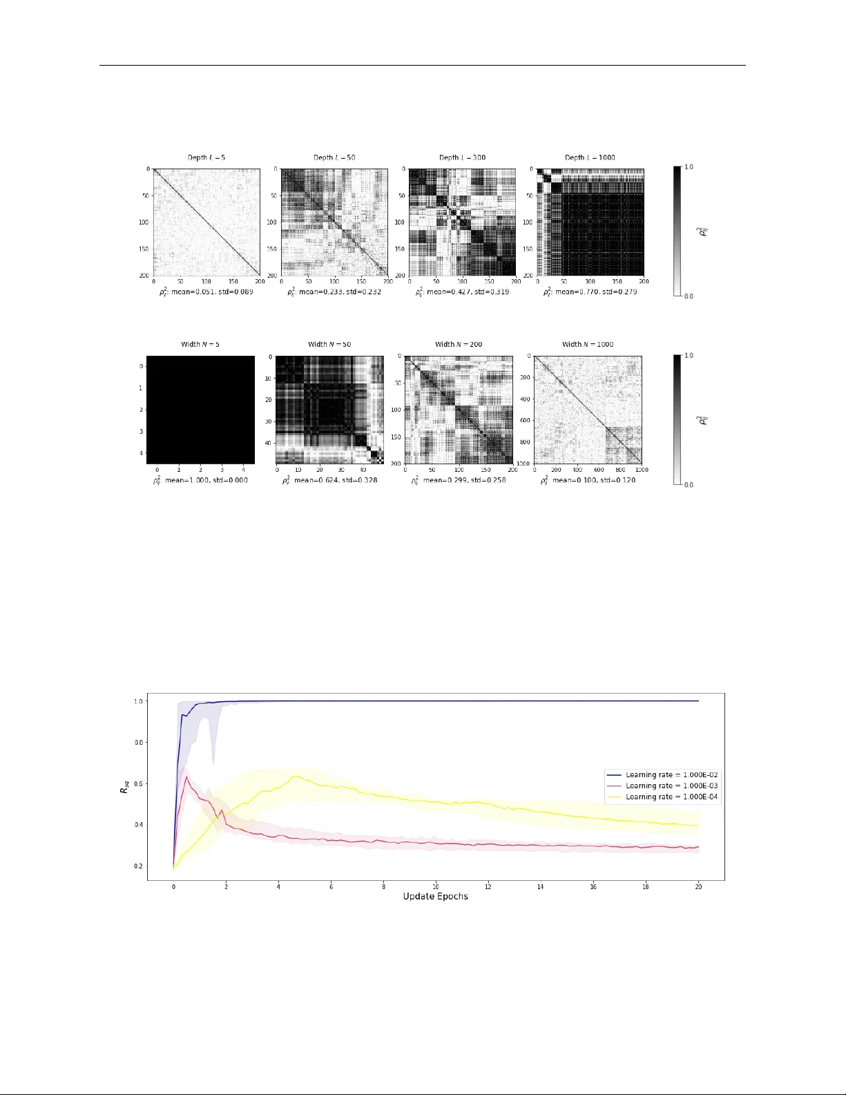
V A N I S H I N G N O D E S : A N O T H E R P H E N O M E N O N T H A T M A K E S T R A I N I N G D E E P N E U R A L N E T W O R K S D I FFI C U L T A P R E P R I N T W en-Y u Chang, Tsung-Nan Lin ∗ October 23, 2019 A B S T R A C T It is well known that the problem of vanishing/e xploding gradients is a challenge when training deep networks. In this paper , we describe another phenomenon, called vanishing nodes , that also increases the difficulty of training deep neural netw orks. As the depth of a neural network increases, the network’ s hidden nodes ha ve more highly correlated beha vior . This results in great similarities between these nodes. The redundancy of hidden nodes thus increases as the network becomes deeper . W e call this problem v anishing nodes, and we propose the metric vanishing node indicator (VNI) for quantitati vely measuring the de gree of vanishing nodes. The VNI can be characterized by the netw ork parameters, which is shown analytically to be proportional to the depth of the network and in versely proportional to the netw ork width. The theoretical results sho w that the ef fecti ve number of nodes vanishes to one when the VNI increases to one (its maximal value), and that vanishing/e xploding gradients and v anishing nodes are two dif f erent challenges that increase the dif ficulty of training deep neural networks. The numerical results from the experiments suggest that the degree of v anishing nodes will become more e vident during back-propagation training, and that when the VNI is equal to 1, the network cannot learn simple tasks (e.g. the XOR problem) ev en when the gradients are neither vanishing nor exploding. W e refer to this kind of gradients as the walking dead gr adients , which cannot help the network conv erge when ha ving a relatively lar ge enough scale. Finally , the experiments sho w that the likelihood of f ailed training increases as the depth of the network increases. The training will become much more difficult due to the lack of netw ork representation capability . 1 Introduction Deep neural networks (DNN) ha ve succeeded in v arious fields, including computer vision [ 13 ], speech recognition [ 12 ], machine translation [ 26 ], medical analysis [ 24 ] and human games [ 22 ]. Some results are comparable to or ev en better than those of human experts. State-of-the-art methods in many tasks have recently used increasingly deep neural network architectures. The performance has impro ved as networks ha ve been made deeper . For example, some of the best-performing models [10, 11] in computer vision hav e included hundreds of layers. Moreov er , recent studies hav e found that as the depth of a neural netw ork increases, problems, such as vanishing or exploding gradients, mak e the training process more challenging. [ 5 , 9 ] in vestigated this problem in depth and suggested that initializing the weights in the appropriate scales can pre vent gradients from v anishing or exploding e xponentially . [ 19 , 21 ] also studied (via mean field theory) ho w vanishing/e xploding gradients arise and provided a solid theoretical discriminant to determine whether the propagation of gradients is v anishing/exploding. Inspired by previous studies, we in vestigated the correlation between hidden nodes and disco vered that a phenomenon that we call vanishing nodes can also affect the capability of a neural network. In general, the hidden nodes of a neural network become highly correlated as the network becomes deeper . A correlation between nodes implies their similarity , and a high degree of similarity between nodes produces redundanc y . Because a sufficiently lar ge number of effecti ve ∗ W en-Y u Chang and Tsung-Nan L in were with the Graduate Institute of Communication Engineering, National T aiwan University , T aipei, T aiwan. V anishing Nodes: Another Phenomenon That Makes Training Deep Neural Netw orks Difficult A P R E P R I N T nodes is needed to approximate an arbitrary function, the redundancy of the nodes in the hidden layers may debilitate the representation capability of the entire network. Thus, as the depth of the network increases, the redundanc y of the hidden nodes may increase and hence affect the netw ork’ s trainability . W e refer to this phenomenon as that of vanishing nodes . In practical scenarios, redundancy of the hidden nodes in a neural network is ine vitable. For e xample, a well-trained feed-forward neural netw ork with 500 nodes in each layer to do the 10-class classification should hav e many highly correlated hidden nodes. Since we only have 10 nodes in the output layer , to achiev e the classification task, the high redundancy of the 500 hidden nodes is not surprising, and is e ven necessary . W e propose a vanishing node indicator (VNI) , which is the weighted av erage of the squared correlation coef ficients, as a quantitati ve metric for the occurrence of v anishing nodes. VNI can be theoretically approximated via the results on the spectral density of the end-to-end Jacobian. The approximation of VNI depends on the network parameters, including the width, depth, distribution of weights, and the activ ation functions, and is shown to be simply proportional to the depth of the network and in versely proportional to the width of the network. When the VNI of a network is equal to 1 (i.e. all the hidden nodes are highly correlated, the redundanc y of nodes is at a maximal le vel), we call this situation network collapse . The representation power is not suf ficient, and hence the network cannot successfully learn most training tasks. The network collapse theorem and its proof are provided to sho w that the ef fectiv e number of nodes vanishes to 1 as the VNI approaches 1. In addition, the numerical results show that back-propagation training also intensifies the correlations of the hidden nodes when we consider a deep network. Also, another weight initialization method is proposed for tweaking the initial VNI of a network to 1 e ven when the network has a relatively small depth. This weight initialization meets the "norm-preserving" condition of [ 5 , 18 ]. Numerical results for this weight initialization method show that when the VNI is set to 1, the netw ork cannot learn simple tasks (e.g. the XOR problem) ev en when v anishing/exploding gradients do not appear . This implies that when the VNI is close to 1, the back-propagated gradients, which are neither v anishing nor exploding, cannot successfully train the network, and hence we call this kind of gradient walking dead gr adients . Finally , we sho w that vanishing/e xploding gradients and v anishing nodes are two dif ferent problems because the two problems may arise from different specific conditions. The experimental results sho w that the likelihood of failed training increases as the depth of the network increases. The training will become much more dif ficult due to the lack of network representation capability . This paper is organized as follows: some related works are discussed in Section 2. The vanishing nodes phenomenon is introduced in Section 3. A theoretical analysis and quantitativ e metric are presented in Section 3. Section 4 compares the problem of vanishing nodes with the problem of vanishing/exploding gradients. Section 6 presents the experimental results and Section 7 presents our conclusions. 2 Related W ork Problems in the training of deep neural networks hav e been encountered in several studies. F or example, [ 5 , 9 ] in vestigated vanishing/exploding gradient propagation and gav e weight initialization methods as the solution. [ 7 ] suggested that vanishing/e xploding gradients might be related to the sum of the reciprocals of the widths of the hidden layers. [ 6 , 3 ] stated that for training deep neural networks, saddle points are more likely to be a problem than local minima. [ 8 , 23 , 10 ] explained the de gradation problem: the performance of a deep neural network degrades as its depth increases. The correlation between the nodes of hidden layers within a deep neural network is the main focus of the present paper , and sev eral kinds of correlations hav e been discussed in the literature. [ 21 ] surve yed the propagation of the correlation between two different inputs after sev eral layers. [ 15 , 25 ] suggested that the input features must be whitened (i.e., zero-mean, unit variances and uncorrelated) to achie ve a faster training speed. Dynamical isometry is one of the conditions that make ultra-deep network training more feasible. [ 20 ] reported the dynamical isometry theoretically ensures a depth-independent learning speed. [ 17 , 18 ] suggested se veral ways to achiev e dynamical isometry for various settings of network architecture, and [ 27 , 1 ] practically trained ultra-deep networks in v arious tasks. 3 V anishing Nodes: Correlation Between Hidden Nodes In this section, the correlations between neurons in the hidden layers are in vestigated. If two neurons are highly correlated (for example, the correlation coef ficient is equal to +1 or − 1 ), one of the neurons becomes redundant. A 2 V anishing Nodes: Another Phenomenon That Makes Training Deep Neural Netw orks Difficult A P R E P R I N T great similarity between nodes may reduce the effecti ve number of neurons within a network. In some cases, the correlation of hidden nodes may disable the entire network. This phenomenon is called vanishing nodes . First, consider a deep feed-forward neural network with depth L . For simplicity of analysis, we assume all layers have the same width N . The weight matrix of layer l is W l ∈ R N × N , the bias of layer l is b l ∈ R N (a column vector), and the common acti vation function of all layers is φ ( · ) : R → R . The input of the network is x 0 , and the nodes at output layer L are denoted by x L . The pre-activ ation of layer l is h l ∈ R N (a column v ector), and the post-acti vation of layer l is x l ∈ R N (a column vector). That is, ∀ l ∈ { 1 , ..., L } , h l = W l x l − 1 + b l , x l = φ ( h l ) . (1) The v ariance of node i is defined as σ 2 i ∆ = E x 0 [( x l ( i ) − x l ( i ) ) 2 ] , and the squared correlation coef ficient ( ρ 2 ij ) between nodes i and j can be computed as ρ 2 ij ∆ = E x 0 [( x l ( i ) − x l ( i ) )( x l ( j ) − x l ( j ) )] 2 E x 0 [( x l ( i ) − x l ( i ) ) 2 ] E x 0 [( x l ( j ) − x l ( j ) ) 2 ] , where ρ 2 ij ranges from 0 to 1 . Nodes x l ( i ) and x l ( j ) are highly correlated only if the magnitude of the correlation coef ficient between them is nearly 1. ρ 2 ij indicates the degree of similarity between node i and node j . If ρ ij is close to +1 or − 1 , then node i can be approximated in a linear fashion by node j . A great similarity indicates redundancy . If the nodes of the hidden layers exhibit great similarity , the ef fectiv e number of nodes will be much lo wer than the original network width. Therefore, we call this phenomenon the vanishing nodes pr oblem . In the following section, we propose a metric to quantitativ ely describe the degree of v anishing of the nodes of a deep feed-forward neural netw ork. A theoretical analysis of this metric indicates that it is proportional to the depth of the network and in versely proportional to the width of the network. This quantity is shown analytically to depend on the statistical properties of the weights and the nonlinear activ ation function. 3.1 V anishing Node Indicator Consider the network architecture defined in eqn. (1) . In addition, the following assumptions are made: (1) The input x 0 is zero-mean, and the features in x 0 are independent and identically distributed. (2) All weight matrices W l in each layer are initialized from the same distribution with variance σ 2 w / N . (3) All the bias vectors b l in each layer are initialized to zero. The input–output Jacobian matrix J ∈ R N × N is defined as the first-order partial deriv ati ve of the output layer with respect to the input layer , which can be rewritten as ∂ x L ∂ x 0 = Q L l =1 D l W l , where D l ∆ = diag ( φ 0 ( h l )) is the deriv ative of the point-wise acti vation function φ at layer l . T o conduct an analysis similar to that of [ 20 ], consider the first-order forward approximation: x L − x L ≈ Jx 0 . Therefore, the covariance matrix of the nodes ( C ∈ R N × N ) at the output layer can be computed as C ∆ = E x 0 [( x L − x L )( x L − x L ) T ] ≈ E x 0 [( Jx 0 )( Jx 0 ) T ] = J E x 0 [ x 0 x T 0 ] J T = σ 2 x JJ T , (2) where σ 2 x is the common variance of the features in x 0 , and the expected v alues are calculated with respect to the input x 0 . For notational simplicity , we omit the subscript x 0 of the expectations in the follo wing equations. It can be easily deri ved that the squared co varianc e of nodes i and j is equal to the product of the squared correlation coefficient and the two v ariances. That is, [ C ( ij ) ] 2 = ρ 2 ij σ 2 i σ 2 j . In this paper , we propose the vanishing node indicator (VNI) R sq to quantitativ ely characterize the degree of vanishing nodes for a giv en network architecture. It is defined as follo ws: R sq ∆ = P N i =1 P N j =1 ρ 2 ij σ 2 i σ 2 j P N i =1 P N j =1 σ 2 i σ 2 j . (3) VNI calculates the weighted av erage of the squared correlation coefficients ρ 2 ij between output layer nodes with non-negati ve weights σ 2 i σ 2 j . Basically , VNI R sq , which ranges from 1 / N to 1 , summarizes the similarity of the nodes at the output layer . If all nodes are independent of each other , the correlation coefficients ρ ij will be 0 (if i 6 = j ) or 1 (if i = j ) and R sq will take on its minimum, which is 1 / N . Otherwise, if all of the output nodes are highly correlated, then all the squared correlation coefficients ρ 2 ij will be nearly 1, and therefore R sq will reach its maximum value 1 . 3 V anishing Nodes: Another Phenomenon That Makes Training Deep Neural Netw orks Difficult A P R E P R I N T Note that the weights σ 2 i σ 2 j in the weighted a verage can be interpreted as the importance of the output-layer nodes i and j . If all of the output layer nodes ha ve equal v ariances, VNI R sq is simply the a verage of the squared correlation coefficients ρ 2 ij . (a) Network width N = 200 (b) Network width N = 500 Figure 1: The results of VNI R sq with respect to network depth L for network widths 200 and 500. The red line is calculated from eqn. (6) , the blue line is computed from eqn. (3) with the input data of zero mean and i.i.d input data, and the green line is computed from eqn. (3) with MNIST data. The VNI R sq expressed in eqn. (6) is very close to the original definition in eqn. (3). W ith the cov ariance matrix defined in eqn. (2) and the formulas for the traces of matrices, VNI R sq can be expressed in terms of the cov ariance matrix as R sq = P N i =1 P N j =1 E x 0 [( x L ( i ) − x L ( i ) )( x L ( j ) − x L ( j ) )] 2 P N i =1 P N j =1 E x 0 [( x L ( i ) − x L ( i ) ) 2 ] E [( x L ( j ) − x L ( j ) ) 2 ] = P N i =1 P N j =1 [ C ( ij ) ] 2 P N i =1 P N j =1 C ( ii ) C ( j j ) = tr ( CC T ) tr ( C ) 2 , (4) where tr ( · ) denotes the trace of a matrix. From eqn. (2) , substituting σ 2 x JJ T for C in eqn. (4) , and noting that tr ( A k ) is equal to the sum of the k th po wers of the eigen v alues of the symmetric matrix A [4], an approximation of R sq can be obtained: R sq ≈ tr ( JJ T JJ T ) tr ( JJ T ) 2 = P N k =1 λ 2 k ( P N k =1 λ k ) 2 = N · m 2 ( N · m 1 ) 2 = m 2 N m 2 1 , (5) where λ k is the k th eigen v alue of JJ T , and m i is the i th moment of the eigen v alues of JJ T . In eqn. (5) , we show that R sq is related to the expected moments of the eigenv alues of JJ T . Because the moments of the eigenv alues of JJ T hav e been analyzed in previous studies [ 18 ], we can leverage the recent results by [ 18 ]: m 1 = ( σ 2 w µ 1 ) L , and m 2 = ( σ 2 w µ 1 ) 2 L L  µ 2 µ 2 1 + 1 L − 1 − s 1  , where σ 2 w / N is the variance of the initial weight matrices, s 1 is the first moment of the series expansion of the S-transform associated with the weight matrices, and µ k is the k th moment of the series expansion of the moment generating function associated with the activ ation functions. If we insert the expressions of m 1 and m 2 into eqn. (5), we can obtain an approximation of the expected VNI: R sq ≈ L N  µ 2 µ 2 1 + 1 L − 1 − s 1  = 1 N + L N  µ 2 µ 2 1 − 1 − s 1  , (6) which shows that VNI is determined by the depth L , the width N , the moments of the activ ation functions µ k and the statistical properties of the weights s 1 . Because R sq ranges from 1 / N to 1 , the approximation in eqn. (6) is more 4 V anishing Nodes: Another Phenomenon That Makes Training Deep Neural Netw orks Difficult A P R E P R I N T accurate when N >> L . Moreover , it can be easily seen that the correlation is in versely proportional to the width N of the network, and proportional to the depth L of the network. T o e v aluate the accuracy of eqn. (6) with respect to the original definition in eqn. (3) , we hav e designed the following experiments. A network width, N ∈ { 200 , 500 } , is set. The network depth L is adjusted from 10 to 100 with the Hard-T anh acti vation function. One thousand data points with the distribution x 0 ∼ Gaussian ( µ x = 0 , σ 2 x = 0 . 1) and 50,000 training images from the MNIST dataset [ 14 ] are fed into the network. In each network architecture, the weights are initialized with scaled-Gaussian distribution [ 5 ] of various random seeds for 100 runs. The R sq calculated from eqn. (3) is then recorded to compute the mean and the standard deviation with respect to various network depths L . The results are shown in Fig. 1 as the blue and green lines denoted “Simulation i.i.d. inputs” and “Simulation MNIST dataset. ” The red line denoted by “Theoretical” is the result calculated from eqn. (6) . This experiment demonstrates that the VNI expressed in terms of the network parameters in eqn. (6) is very close to the original definition in eqn. (3) . Similar results are obtained with different acti v ation functions (e.g., Linear , ReLU) and different weight initializations (e.g., scaled uniform distribution). Fig. 2 plots the squared correlation coefficients between output nodes, which are ev aluated with 50,000 training images in the MNIST dataset [ 14 ] for various network architectures. White indicates no correlation, and black means that ρ 2 ij = 1 . Fig. 2 (a) plots the squared correlation coefficients for four architectures with the same network width ( N = 200 ) at different depths (5, 50, 300, and 1000). Fig. 2 (b) shows the architectures with the same depth ( L = 100 ) and different widths (5, 50, 200, 1000). This shows that the vanishing node phenomenon becomes evident with increasing depth and is in versely proportional to the width. 3.2 Network collapse When the VNI of a network is equal to 1 (i.e. all the hidden nodes are highly correlated, the redundancy of the nodes is at a maximal lev el), and so the network collapses to only one effecti ve node. The representation power is not suf ficient, and hence the netw ork cannot successfully learn most training tasks, e.g., classification tasks with more than two classes, or non-linearly separable classification tasks. As theoretical evidence for this claim, we present the network collapse theor em : Theorem 1 (Netw ork collapsing) . The ef fective number of nodes becomes 1 when the VNI R sq is 1. Pr oof. First, the N random variables of the values of the nodes in a hidden layer are defined as { X 1 , X 2 , ..., X N } . W ithout loss of generality , we assume that each X i follows a N (0 , 1) distribution. Therefore, the cov ariance matrix of the random vector [ X 1 , X 2 , ..., X N ] T is C =     1 ρ 12 · · · ρ 1 N ρ 21 1 · · · ρ 2 N . . . . . . . . . . . . ρ N 1 ρ N 2 · · · 1     , (7) where C ij = E [( X i − X i )( X j − X j )] as defined in eqn. (2) , ρ ij is the correlation coefficient between X i and X j , and hence C is a symmetric matrix. By the definition of the VNI R sq from eqn. (3), the R sq can be represented as R sq = P N i =1 P N j =1 ρ 2 ij N 2 = tr ( CC T ) N 2 = 1 N 2 tr ( C 2 ) . (8) Let the eigen v alues of C be λ 1 , λ 2 , . . . , λ N . By the relation between trace of a matrix and its eigen values, we ha ve N X i =1 λ i = tr ( C ) = N N X i =1 λ 2 i = tr ( C 2 ) = N 2 R sq . (9) T o relate R sq with the redundancy of the random v ariables, a method for measuring the redundancy is needed. From a principle component analysis (PCA), the eigen value of C can represent the energy (i.e. the variance) associated with each eigen vector . Therefore, we can use the distribution of the eigen v alues λ i to determine the proportion of redundant components, and hence the effecti ve number of nodes can be ev aluated. Similar to PCA, we first rearrange the order of 5 V anishing Nodes: Another Phenomenon That Makes Training Deep Neural Netw orks Difficult A P R E P R I N T the eigen values λ i so that λ 1 ≥ λ 2 ≥ · · · ≥ λ N ≥ 0 . W e suppose gi ven a constant, ε ∈ (0 , 1) , the effective thr eshold ratio of the eigen values. That is, if λ i ≥ ελ 1 , then we say that the i th component λ i is ε -effecti ve. Otherwise, the i th component λ i is said to be redundant. W e introduce a ne w metric called the ε -ef fectiv e number of nodes ( ε -ENN): ε -ENN ≡ N ε e ∆ = max ( { t ∈ N : λ t ≥ ελ 1 } ) . (10) That is, ε -ENN is the maximum number of ε -effecti ve nodes. As in eqn. (9) , the constraints on λ i are al- ready deri ved. Also, it is intuiti ve that the maximum in eqn. (10) can simply be attained with eigenv alues { λ 1 , ελ 1 , . . . , ελ 1 , 0 , . . . , 0 . . . , 0 } , where there are ( N ε e − 1) ελ 1 and ( N − N ε e ) zeros. Inserting these eigenv al- ues into eqn. (9), we get λ 1 + ( N ε e − 1) ελ 1 = N λ 2 1 + ( N ε e − 1)( ελ 1 ) 2 = N 2 R sq . (11) Inserting the first equation in eqn. (11) into the second one, we get [1 + ( N ε e − 1) ε ] 2 =  N λ 1  = 1 + ( N ε e − 1) ε 2 R sq , (12) which is a solvable quadratic equation. Making use of the condition R sq = 1 , we hav e [1 + ( N ε e − 1) ε ] 2 = 1 + ( N ε e − 1) ε 2 ⇒ ( N ε e − 1)[( N ε e − 2) ε + 2] = 0 ⇒ N ε e = 1 (13) The solution for N ε e in eqn. (12) is 1 (no matter the v alue of ε ). Therefore, the ε -ef fectiv e number of nodes N ε e becomes only 1 when the VNI R sq is 1. Therefore, when the VNI approaches 1, the network de grades to a single perceptron, and hence the representation po wer of the network is insufficient to solve practical tasks (e.g., classification tasks with more than tw o classes or non-linearly separable classification tasks). 3.3 Impact of back-propagation In Section 3.1, we showed that the correlation of a network will increase as the depth L increases; in this section, we exploit the manner in which the back-propagation training process will influence the network correlation by the following e xperiments. First, the same architecture defined in eqn. (1) , with L = 100 , N = 500 , tanh activ ation, and scaled Gaussian initialization [ 5 ], is used. The network is then trained on the MNIST dataset [ 14 ] and optimized with stochastic gradient descent (SGD) with a batch size of 100. The network is trained with three different learning rates for dif ferent seeds to initialize the weights for 20 runs. W e then record the quartiles of VNI ( R sq ) with respect to the training epochs, as shown in Fig. 3. The boundaries of the colored areas represent the first and the third quartiles (i.e., the 25th and the 75th percentiles), and the line represents the second quartile (i.e., the median) of R sq ov er 20 trials. This shows that in some cases, VNI increases to 1 during the training process, otherwise VNI grows lar ger initially , and then decreases to a value which is larger than the initial VNI. A sev ere intensification of VNI may occur , as shown by the blue line, which is trained at the learning rate of 10 − 2 . Moreover , we observe that training will become much more dif ficult due to a lack of network representation capability as VNI R sq approaches 1. Further discussion is provided in Section 6 to in vestigate, by the use of various training parameters, the impact of VNI. 4 Comparison with Exploding/V anishing Gradients In this section, we explore whether the v anishing nodes phenomenon arises from the problem of exploding/v anishing gradients. Exploding/v anishing gradients in deep neural networks are a problem regarding the scale of forward- propagated signals and back-propagated gradients, which e xponentially explode/v anish as the networks gro ws deeper . W e perform a theoretical analysis of exploding/v anishing gradients and show analytically the dif ference between them and the newly identified problem of v anishing nodes. 6 V anishing Nodes: Another Phenomenon That Makes Training Deep Neural Netw orks Difficult A P R E P R I N T (a) Network width N = 200 (c) Network depth L = 100 Figure 2: The magnitudes of correlation coefficient ρ ij between output nodes. The black color means ρ 2 ij = 1 while the white color indicates ρ 2 ij = 0 . The top row sho ws that the correlation is positiv ely related to the network depth L , and the bottom row that the correlation is negati vely related to the network width N . Note that we have rearranged the node index to cluster the correlated nodes. Figure 3: Sev ere intensification of VNI (increases to 1) may occur , as shown by the blue line, which is trained with a learning rate of 10 − 2 . Otherwise VNI rises initially , and then decreases to a value which is lar ger than the initial VNI. 7 V anishing Nodes: Another Phenomenon That Makes Training Deep Neural Netw orks Difficult A P R E P R I N T As in a pre vious study [ 5 ], we use the v ariances of the hidden nodes to ev aluate the scales of the back-propagated gradients. Consider the model and the assumptions in Section 3 and an additional assumption: the gradient ∂ C ost ∂ x L of the output layer is a zero-mean i.i.d. random (row) v ector . That is, E [ x 0 x 0 T ] = σ 2 x · I and E h ∂ C ost ∂ x L  T ∂ C ost ∂ x L i = σ 2 y · I , where σ 2 x and σ 2 y are defined as the variances of the input layer nodes and output layer gradients, respectiv ely . Consider the variances V ar [ x L ] and V ar h ∂ C ost ∂ x 0 i of the gradients of the output nodes and the input nodes, respectively . The phenomena of exploding/vanishing gradients occur only if the scales of the forward and backward propagation exponentially increase or decrease as the depth increases. This means that the magnitude of the gradients will be bounded if we can prev ent the scales of forward and backward propag ation from exploding or v anishing. According to the assumptions in Section 3 and eqn. (2) , we can approximate the shared scalar v ariance of all output nodes V ar [ x L ] ∈ R and the shared scalar variance of all input gradients V ar h ∂ C ost ∂ x 0 i ∈ R by V ar [ x L ] = E [( x L − x L ) T ( x L − x L )] / N ≈ E [( Jx 0 ) T Jx 0 ] / N = E [ tr ( J T Jx 0 x T 0 )] / N = σ 2 x · tr ( J T J ) / N (14) V ar h ∂ C ost ∂ x 0 i = E h ∂ C ost ∂ x 0 − ∂ C ost ∂ x 0  ∂ C ost ∂ x 0 − ∂ C ost ∂ x 0  T i. N = E h ∂ C ost ∂ x L J  ∂ C ost ∂ x L J  T i. N = σ 2 y · tr ( J T J ) / N , (15) where the chain rule for back-propagation, ∂ C ost ∂ x 0 = ∂ C ost ∂ x L ∂ x L ∂ x 0 = ∂ C ost ∂ x L J , is used, and the shared scalar variance of a vector is the av erage of the variances of all its components. Also, it is already known that tr ( J T J ) = N · m 1 = N · ( σ 2 w µ 1 ) L . Thus, we have V ar [ x L ] = σ 2 x ( σ 2 w µ 1 ) L and V ar h ∂ C ost ∂ x 0 i = σ 2 y ( σ 2 w µ 1 ) L , where σ 2 w = N · V ar [ W ij ] , and µ 1 is the first moment of the nonlinear activ ation function. It is obvious that the variances of both forward and backward propagation will neither e xplode nor vanish if and only if ( σ 2 w µ 1 ) = 1 . For the weight gradient of the hidden layer l , the variance can be used to measure the scale distribution. Because ∂ C ost ∂ W l = x l − 1 · ∂ C ost ∂ h l and both x l − 1 and ∂ C ost ∂ h l are assumed to be zero-mean, the v ariance of the weight gradient can be ev aluated as V ar h ∂ C ost ∂ W l i = V ar [ x l − 1 ] · V ar h ∂ C ost ∂ h l i ≈ σ 2 x σ 2 y ( σ 2 w µ 1 ) L − 1 , (16) where we can ev aluate V ar [ x l − 1 ] and V ar h ∂ C ost ∂ h l i using the results of the forward/backward v ariance propagation and split the entire network into two sub-networks. One sub-network has the input layer x 0 and output layer x l − 1 , and the other sub-network has the input layer x l and the output layer x L . Note that eqn. (16) also implies that if, and only if, ( σ 2 w µ 1 ) = 1 , the weight gradients will never e xplode or v anish. Ho wev er , eqn. (6) sho ws that VNI ( R sq ) may still increase with the depth of the network e ven if ( σ 2 w µ 1 ) = 1 . That is, the occurrence of the vanishing nodes becomes e vident when ( µ 2 /µ 2 1 − 1 − s 1 ) is close to 1, whereas vanishing/exploding gradients occur when ( σ 2 w µ 1 ) is far from 1. If the network’ s initialization parameter is appropriately set, so that ( σ 2 w µ 1 ) is close to 1, R sq may still tend to 1 due to the network depth, the activation function, and the weight distribution. Therefore, from eqn. (6) and eqn. (16) , it is clear that the problem of vanishing nodes may occur regardless of whether there are exploding/v anishing gradients. 5 In voke the T raining Difficulty of V anishing Nodes In this section, a weight initialization method is introduced to make a shallo w network (with depth around 50) address the difficulty of training. This method will satisfy the norm-pr eserving condition, ( σ 2 w µ 1 ) = 1 , mentioned in Section 4. 8 V anishing Nodes: Another Phenomenon That Makes Training Deep Neural Netw orks Difficult A P R E P R I N T W ith this kind of weight initialization, the network cannot ev en learn a simple task, such as the XOR problem. Also, an analysis on the failed training is provided. 5.1 T weaking the VNI In Section 3, we have already shown that when the VNI approaches 1, the network has a representation power that is inefficient to accomplish practical tasks. Here, we provide a weight initialization method which satisfies the norm-preserving condition introduced in Section 4, which can help us to tweak the initial VNI of a network to nearly 1: Input: The dimension of the input v ector , N i The dimension of the output vector , N o The dimension of the bottleneck vector , N b Output: Initialized weight matrix, W with dimensions ( N o , N i ) 1: Randomly sample a matrix U with dimensions ( N b , N i ) with zero mean and unit variance 2: Randomly sample a matrix V with dimensions ( N o , N b ) with zero mean and unit variance 3: Ev aluate c W = V · U 4: A verage number of inputs and outputs: N mean = ( N i + N o ) / 2 5: Normalization: W = c W / √ N b · N mean Note that the normalization obeys the norm-preserving constraint introduced by [5]. The bottleneck dimension N b is used to make the network much “leaner”. That is, when a small bottleneck dimension N b is chosen, the initial effecti ve number of nodes will be smaller without modifying the network architecture, and hence we can hav e the VNI nearly 1 with a shallower netw ork architecture. If the bottleneck dimension N b is set to 1 , then due to Step 3 of the weight initialization method, the rank of the weight matrix W will become only 1. That is, the weight matrix W will have only 1 non-zero eigenv alue. By eqn. (5) , if all the weight matrices of a network are initialized by this method, then the VNI R sq will tend to 1. Therefore, we can tune the netw ork to make the VNI tend to 1 ev en when the depth is not large. An architectural vie w of the weight initialization method is provided in Fig. 4. It is shown that if the weight matrices are initialized by the introduced method, the effecti ve number of nodes will become only N b . If N b is set to 1, then the initial VNI R sq of the network will increase to 1. The simulation results are provided as numerical evidences for this. The networks are examined by the AND and the XOR tasks, where we use 2 or 4 bits as input data and the AND/XOR results of the input data as the output label (with 2 or 4 classes), which can be written as y 2 and = x 0 AND x 1 , y 4 and = ( x 0 AND x 1 ) · 2 + ( x 2 AND x 3 ) and y xor = x 0 X OR x 1 . A successful training is defined as when the testing accuracy exceeds 0.99 (for MNIST , it’ s defined as 0.9) in 100 epochs over 20 runs. The AND task can be viewed as a linearly-separable classification task, while the XOR task is a non-linearly-separable problem. In the simulation, the network depth L is set to 50 with the tanh activ ation function, the network width N is set to 500, the bottleneck dimension N b is set to 30, and the network is trained with a 0 . 01 learning rate. The initial VNI of a network is tweaked to 1 by initializing the weight matrices with rank = N b . It is shown in T able 1 that compared with networks with initial VNI 6 = 1 , the networks to initial VNI = 1 hav e insuf ficient representation power to learn either the XOR or the MNIST tasks. Also, the metric σ 2 w µ 1 is nearly 1 throughout the entire training, which implies that the failures are not caused by the v anishing/exploding gradients problem. That is, the vanishing nodes are indeed a problem when the VNI is nearly 1. T able 1: T weaking the initial VNI to 1. T asks # of classes Gaussian Init. Initial VNI = 1 AND 2 Success(VNI 6 = 1) Success(VNI = 1) AND 4 Success(VNI 6 = 1) Fail(VNI = 1) XOR 2 Success(VNI 6 = 1) Fail(VNI = 1) MNIST 10 Success(VNI 6 = 1) Fail(VNI = 1) 5.2 W alking dead gradients when the VNI is 1 T o analyze the failure of the training in the previous subsection, we first define a kind of gradients, to be referred to as walking dead gradients. The phrase “walking dead” consists of two words: “walking” means the gradients, which are used to update the weight matrices of the network, still have a non-vanishing value, but “dead” implies that the 9 V anishing Nodes: Another Phenomenon That Makes Training Deep Neural Netw orks Difficult A P R E P R I N T (a) Ordinary weight init. (b) The introduced weight init. Figure 4: An architectural vie w of the introduced weight initialization. Compared with ordinary weight initialization methods, the introduced weight initialization makes the initial weight matrix hav e a smaller rank N b . If the parameter N b is set to 1, then the effecti ve number of hidden nodes will reduce to 1, which implies that the VNI R sq of the network will increase to 1. gradients cannot successfully train the network. W e observe that if the weight matrices are initialized as in the previous subsection, the initial VNI will be close to 1. Below , the details of the training are provided in T able 1. T able 1 shows that although the network architectures (see Fig. 4), the training en vironments, and the scales of the back-propagated gradients are the same, the Gaussian initialized weight matrices can learn all the tasks while the network with initial VNI = 1 fails and cannot escape from the occurrence of vanishing nodes. W alking : As discussed in Section 4, we have sho wn that the values of the gradients will not vanish if the initial weight condition ( σ 2 w µ 1 = 1 ) is met. In the introduced weight initialization, it is obvious that the variance of the obtained weight matrix will be V ar [ W ] = N b · V ar [ u ] · V ar [ v ] N b · N mean , which implies that the parameter σ 2 w will become V ar [ W ] · N mean = 1 . In Fig. 5, we would like to show that the scales of the back-propagated gradients of the scaled-Gaussian initialized network are similar to those of the network with initial VNI = 1. As in T able 1, the network depth L is set to 50 with tanh activ ation function, the network width N is set to 500, the bottleneck dimension N b is set to 30, and the network is trained with 0 . 01 learning rate. W e record the gradient values at the input layer nodes ov er 20 runs, and then e valuate the log-scales of the gradients. The log-ratio of the gradients between two different initial weights are provided in Fig. 5. It can be seen that the gradients of both the scaled-Gaussian initialized network and the network with initial VNI = 1 hav e similar scales, which implies that the vanishing/e xploding problems do not occur . That is, the gradients still provide information from the back-propagation, but the gradients somehow cannot modify the network to ward a successful model. Dead : In T able 1, the network architectures, optimization methods and the training en vironments for two initialization methods are totally the same. Ho wev er for the XOR task, the scaled-Gaussian initialized network can reach 100% testing accuracy in around 5 epochs, while the testing accuracy of the network with initial VNI = 1 cannot exceed 90% for ov er 100 epochs. That is, the representation power of the network with initial VNI = 1 is not suf ficient to learn the task, and therefore the network is called a dead network. 10 V anishing Nodes: Another Phenomenon That Makes Training Deep Neural Netw orks Difficult A P R E P R I N T Figure 5: The log ratio of the back-propagated gradients between the scaled-Gaussian initialized network and the network with initial VNI = 1. (a) T anh, Scaled Gaus- sian Init. (b) ReLU, Scaled Gaus- sian Init. (c) T anh, Orthogonal Init. (d) ReLU, Orthogonal Init. (e) T anh, Householder Param. Figure 6: Probability of successful training for different network depths L and learning rates α (SGD optimizer). Black denotes a zero probability of successful training. 6 Experiments T o empirically explore the ef fects of the phenomenon of v anishing nodes on the training of deep neural networks, we hav e performed experiments with the training tasks on the MNIST dataset [ 14 ]. Because the purpose is to focus on the problem of vanishing nodes, the networks are designed so that v anishing/exploding gradients will ne ver occur; that is, they are initialized with weights ( σ 2 w µ 1 = 1 ). The network is trained with a batch size of 100. The number of successful trainings for a total of 20 runs is recorded to reflect the influence of vanishing nodes on the training process, which may lead to insuf ficient network representation capability , as shown in Fig. 3. A successful training is considered to occur when the training accuracy exceeds 90% within 100 epochs. The network depth L ranges from 25 to 500 , and 11 V anishing Nodes: Another Phenomenon That Makes Training Deep Neural Netw orks Difficult A P R E P R I N T the network width N is set to 500 . The learning rate α ranges from 10 − 4 to 10 − 2 with the SGD algorithm. Both L and α are uniformly distributed on the logarithmic scale. The experiments were performed in the MXNet frame work[2]. Considering that the MNIST dataset is too simple a task, we would say that we intentionally chose an easy training task in order to claim that when the VNI increases to 1, the deep netw ork cannot e ven learn a simple task. If vanishing nodes make the network f ail at such a simple task, then a more challenging task should be ev en less possible to carry out. Fig. 6 shows the results of two different activ ation functions (T anh/ReLU) with two different weight initializations (scaled-Gaussian/orthogonal from [ 20 ]). When a network with tanh acti vation functions is initialized with orthogonal weights, the term of ( µ 2 /µ 2 1 − 1 − s 1 ) in eqn. (6) becomes zero. Therefore, its R sq will be the minimum value ( 1 / N ) and will not depend on the network depth. For the other network parameters, ( µ 2 /µ 2 1 − 1 − s 1 ) will not equal zero, and R sq still depends on the network depth. The experimental results sho w that the likelihood of a f ailed training is high when the depth L and the learning rate are large. In addition, the corresponding R sq of failed cases becomes nearly 1 , which causes a lack of network representation power . This implies that the vanishing nodes problem is the main reason that the training fails. A comparison of Fig. 6c with the other three results shows clearly that the networks with the minimum R sq value ha ve the highest successful training probability . Shallow network architectures can tolerate a greater learning rate, which is why the vanishing node problem has been ignored in man y networks with small depths. In a deep network, the learning rate should be set to small v alues to prev ent R sq from increasing to 1. The reason why the behavior of R sq is affected by the learning rate α remain unexplained, suggesting the need for further in vestigations to better understand the relation between the learning rate and the dynamics of R sq . A high learning rate will cause R sq to be se verely intensified to nearly 1, and the representation capability of the network will be reduced to that of a single perceptron, which is the main reason that the training fails. Further analyses of the cause of failed training are provided in the follo wing subsection. 6.1 The cause of failed training In this subsection, we analyze the reason why failed training occurs from two perspectiv es: vanishing/exploding gradients and vanishing nodes. First, the quantity σ 2 w (the v ariance of weights at each layer ) of trained models is ev aluated. There are a total of 31,680 runs in the experiments, including 13,101 failures and 18,579 successes. Detailed information is presented in T able 2. The quantity σ 2 w µ 1 for measuring the degree of v anishing/exploding gradients is presented in Fig. 7 and Fig. 8 for successful networks and failed networks. The two figures display box and whisker plots to represent the distribution of σ 2 w µ 1 at each network layer , and the horizontal axis indicates the depth of the trained network. The results show that both successful and failed networks ha ve σ 2 w µ 1 near one. This indicates that both successful and failed models satisfy a condition of that prev ents the networks from ha ving v anishing/exploding gradients. Second, the differences in R sq between successful and failed networks are displayed in Fig. 9. The horizontal axis indicates the R sq of trained models ev aluated by eqn. (3) , and the vertical axis represents the binned frequencies of R sq . The blue histogram represents the R sq of the failed networks, and the orange histogram represents the R sq of the successful networks. The R sq of the failed models ranges from 0.9029 to 1.0000 with a mean of 0.9949 and a standard de viation of 0.0481, and that of the successful models ranges from 0.1224 to 0.9865 with a mean of 0.3207 and a standard de viation of 0.1690. The figure shows that the R sq of the failed networks mainly cluster around 1, but those of the successful networks are widely distributed. From the analysis shown in Figs. 7, 8 and 9, it is clear that the vanishing nodes ( R sq reaches 1) is the main cause which makes the training fail. In Fig. 6c, the dark region at the top right corner reveals that although the weight matrices are initially orthogonal, after the training they turn out to be non-orthogonal with a VNI close to 1. As a motiv ation, we restrict the weights to orthogonal matrices by the Householder parameterization[16]. 6.2 Orthogonal constraint: The Householder parametrization An n -dimensional weight matrix follo wing the Householder parametrization can be represented by the product of n orthogonal Householder matrices[ 16 ]. That is, W = H n · H n − 1 · · · H 1 , where the H i are defined by I − 2 v i v T i and the v i are vectors with unit norm. The results of the Householder parameterization are provided in Fig. 6e, where the disappearance of the dark region implies that a successful training can be attained if the weight matrices remain orthogonal during the training process. Also, we provide other results in T able 3. It shows that for the MNIST classification, there is training success for 20 runs e ven with a lar ge learning rate ( 10 − 2 ) and a lar ge network depth ( 500 ) are used, which the orthogonal initialization cannot attain. This sho ws that forcing the VNI be small during the whole of the training process can pre vent the network from failing at training, and it also implies that the failure cases are indeed caused by the v anishing nodes. 12 V anishing Nodes: Another Phenomenon That Makes Training Deep Neural Netw orks Difficult A P R E P R I N T Figure 7: Box and whisker plot of σ 2 w µ 1 for networks with successful training. There are 18,579 successful runs. Figure 8: Box and whisker plot of σ 2 w µ 1 for networks with failed training. There are 13,101 failed runs. 7 Conclusion The phenomenon of vanishing nodes has been in vestigated as another challenge when training deep networks. Like the v anishing/exploding gradients problem, v anishing nodes also make training deep networks dif ficult. The hidden nodes in a deep neural network become more correlated as the depth of the network increases, as the similarity between the hidden nodes increases. Because a similarity between nodes results in redundancy , the effecti ve number of hidden nodes in a network decreases. This phenomenon is called vanishing nodes . 13 V anishing Nodes: Another Phenomenon That Makes Training Deep Neural Netw orks Difficult A P R E P R I N T Figure 9: Histogram of R sq of failed/successful networks. Optimizer Activ ation W eight Init. No. of Failure No. of Success SGD T anh Scaled Gaussian 712 1268 ReLU 1775 205 T anh Orthogonal 62 1918 ReLU 882 1098 SGD+momentum T anh Scaled Gaussian 982 998 ReLU 1140 840 T anh Orthogonal 546 1434 ReLU 1044 936 Adam T anh Scaled Gaussian 609 1371 ReLU 723 1257 T anh Orthogonal 354 1626 ReLU 1465 515 RMSProp T anh Scaled Gaussian 763 1217 ReLU 827 1153 T anh Orthogonal 453 1527 ReLU 764 1216 T able 2: The detailed numbers of successful and failed runs. T o measure the degree of v anishing nodes, the vanishing nodes indicator (VNI) is proposed. It is shown theoretically that the VNI is proportional to the depth of the network and in versely proportional to the width of the network, which is consistent with the e xperimental results. Also, it is mathematically pro ven that when the VNI equals 1, the ef fecti ve number of nodes of the network v anishes to 1, and hence the network cannot learn some simple tasks. Moreov er , we explore the dif ference between vanishing/exploding gradients and vanishing nodes, and another weight initialization method which pre vents the network from ha ving vanishing/exploding gradients is proposed to tweak the initial VNI to 1. The numerical results of the introduced weight initialization reveal that when the VNI is set to 1, a relati vely shallo w network may still not to be able to not accomplish an easy task. The back-propagated gradients of the network still ha ve suf ficient magnitudes, but cannot make the training succeed, and therefore we say that the gradients are walking dead . Finally , experimental results sho w that the training f ails when there are v anishing nodes, b ut that if an orthogonal weight parametrization is applied to the network, the problem of vanishing nodes will be eased, and the training of the deep neural network will succeed. This implies that the vanishing nodes are indeed the cause of the difficulty of the training. 14 V anishing Nodes: Another Phenomenon That Makes Training Deep Neural Netw orks Difficult A P R E P R I N T T able 3: Forcing the weights to remain orthogonal throughout the entire training process. Number of layers L Scaled Gaussian Init. Scaled Orthogonal Init. Householder Parametrization 50 Success (VNI 6 = 1 ) Success (VNI 6 = 1 ) Success (VNI 6 = 1 ) 200 Fail (VNI = 1 ) Success (VNI 6 = 1 ) Success (VNI 6 = 1 ) 500 Fail (VNI = 1 ) Fail (VNI = 1 ) Success (VNI 6 = 1 ) Acknowledgement This research is partially supported by the "Cyber Security T echnology Center" of National T aiwan University (NTU), sponsored by the Ministry of Science and T echnology , T aiwan, R.O.C. under Grant no. MOST 108-2634-F-002-009. References [1] Minmin Chen, Jef frey Pennington, and Samuel S. Schoenholz. Dynamical isometry and a mean field theory of RNNs: Gating enables signal propagation in recurrent neural networks. In Pr oceedings of the 35th International Confer ence on Machine Learning , v olume 80, pages 873–882, 2018. [2] T ianqi Chen, Mu Li, Y utian Li, Min Lin, Naiyan W ang, Minjie W ang, T ianjun Xiao, Bing Xu, Chiyuan Zhang, and Zheng Zhang. MXNet: A fle xible and efficient machine learning library for heterogeneous distrib uted systems. [3] Y ann Dauphin, Razvan P ascanu, Caglar Gulcehre, Kyunghyun Cho, Surya Ganguli, and Y oshua Bengio. Identify- ing and attacking the saddle point problem in high-dimensional non-con vex optimization. In Advances in Neural Information Pr ocessing Systems 27 , pages 2933–2941, 2014. [4] F .R. Gantmacher . The Theory of Matrices . Chelsea Pub. Co., Ne w Y ork, 1960. [5] Xavier Glorot and Y oshua Bengio. Understanding the difficulty of training deep feedforward neural networks. In Pr oceedings of the Thirteenth International Conference on Artificial Intelligence and Statistics , volume 9, pages 249–256, 2010. [6] Ian J. Goodfellow , Oriol V inyals, and Andrew M. Sax e. Qualitativ ely characterizing neural network optimization problems. In International Confer ence on Learning Repr esentations, 2014 , 2015. [7] Boris Hanin. Which neural net architectures giv e rise to exploding and v anishing gradients? Neural Information Pr ocessing Systems , 2018. [8] Kaiming He and Jian Sun. Conv olutional neural networks at constrained time cost. In The IEEE Confer ence on Computer V ision and P attern Recognition , pages 5353–5360, June 2015. [9] Kaiming He, Xiangyu Zhang, Shaoqing Ren, and Jian Sun. Delving deep into rectifiers: Surpassing human-lev el performance on ImageNet classification. In IEEE International Confer ence on Computer V ision , 2015. [10] Kaiming He, Xiangyu Zhang, Shaoqing Ren, and Jian Sun. Deep residual learning for image recognition. In Pr oceedings of the IEEE Conference on Computer V ision and P attern Recognition , pages 770–778, 2016. [11] Kaiming He, Xiangyu Zhang, Shaoqing Ren, and Jian Sun. Identity mappings in deep residual networks. In Eur opean Conference on Computer V ision , pages 630–645. Springer-V erlag, 2016. [12] Geoffre y Hinton, Geor ge Dahl, Abdel-Rahman Mohamed, Na vdeep Jaitly , Andrew Senior , V incent V anhoucke, Brian Kingsbury , and T ara Sainath. Deep neural networks for acoustic modeling in speech recognition. IEEE Signal Pr ocessing Magazine , 29:82–97, 2012. [13] Alex Krizhe vsky , Ilya Sutske ver , and Geoffry E. Hinton. Imagenet classification with deep con volutional neural networks. Advances in Neural Information Pr ocessing Systems , pages 1106–1114, 2012. [14] Y ann Lecun, Léon Bottou, Y oshua Bengio, and Patrick Haf fner . Gradient-based learning applied to document recognition. Pr oceedings of the IEEE , 86(11):2278–2324, 1998. [15] Y ann LeCun, Léon Bottou, Gene viev e B. Orr , and Klaus-Robert Müller . Efficient BackPr op , pages 9–50. Springer- V erlag, Berlin, 1998. This book is an outgrowth of a 1996 NIPS workshop. [16] Rajbir Nirwan and Nils Bertschinger . Rotation in variant householder parameterization for Bayesian PCA. In Kamalika Chaudhuri and Ruslan Salakhutdinov , editors, Proceedings of the 36th International Conference on Machine Learning , v olume 97, pages 4820–4828. PMLR, 09–15 Jun 2019. [17] Jeffre y Pennington and Samuel S. Schoenholz. Resurrecting the sigmoid in deep learning through dynamical isometry: Theory and practice. Advances in Neural Information Pr ocessing Systems , 30:4788–4798, 2017. 15 V anishing Nodes: Another Phenomenon That Makes Training Deep Neural Netw orks Difficult A P R E P R I N T [18] Jeffre y Pennington, Samuel S. Schoenholz, and Surya Ganguli. The emergence of spectral uni versality in deep networks. In International Confer ence on Artificial Intelligence and Statistics, AIST ATS 2018, 9–11 April 2018, Playa Blanca, Lanzar ote, Canary Islands, Spain , pages 1924–1932, 2018. [19] Ben Poole, Subhaneil Lahiri, Maithra Raghu, Jascha Sohl-Dickstein, and Surya Ganguli. Exponential expressi vity in deep neural networks through transient chaos. Neural Information Pr ocessing Systems , 2016. [20] Andre w M. Saxe, James L. McClelland, and Surya Ganguli. Exact solutions to the nonlinear dynamics of learning in deep linear neural networks. In International Conference on Learning Repr esentations , 2013. [21] Samuel S. Schoenholz, Justin Gilmer , Surya Ganguli, and Jascha Sohl-Dickstein. Deep information propagation. In International Confer ence on Learning Repr esentations , 2017. [22] David Silver , Aja Huang, Chris J. Maddison, Arthur Guez, Laurent Sifre, George va n den Driessche, Julian Schrittwieser , Ioannis Antonoglou, V eda Panneershelv am, Marc Lanctot, Sander Dieleman, Dominik Grewe, John Nham, Nal Kalchbrenner , Ilya Sutske ver , Timoth y Lillicrap, Madeleine Leach, Koray Ka vukcuoglu, Thore Graepel, and Demis Hassabis. Mastering the game of go without human knowledge. Natur e , 529(7587):484–489, 2016. [23] Rupesh K umar Sriv astava, Klaus Gref f, and Jurgen Schmidhuber . Highway networks. [24] Nima T ajbakhsh, Jae Y . Shin, Suryakanth R. Gurudu, R. T odd Hurst, Christopher B. Kendall, Michael B. Gotway , and Jianming Liang. Con volutional neural networks for medical image analysis: Full training or fine tuning? IEEE T ransactions on Medical Imaging , 35(5):1299–1312, 2016. [25] Simon Wiesler and Hermann Ney . A conv ergence analysis of log-linear training. In Advances in Neural Information Pr ocessing Systems 24 , pages 657–665, 2011. [26] Y onghui W u, Mike Schuster , Zhifeng Chen, Quoc V . Le, Mohammad Norouzi, W olfgang Macherey , Maxim Krikun, Y uan Cao, Qin Gao, Klaus Machere y , Jeff Klingner , Apurv a Shah, Melvin Johnson, Xiaobing Liu, Lukasz Kaiser , Stephan Gouws, Y oshikiyo Kato, T aku Kudo, Hideto Kazawa, K eith Stev ens, George Kurian, Nishant Patil, W ei W ang, Cliff Y oung, Jason Smith, Jason Riesa, Alex Rudnick, Oriol V inyals, Gre g Corrado, Macduf f Hughes, and Jeffre y Dean. Google’ s neural machine translation system: Bridging the gap. [27] Lechao Xiao, Y asaman Bahri, Jascha Sohl-Dickstein, Samuel S. Schoenholz, and Jeffrey Pennington. Dynamical isometry and a mean field theory of CNNs: Ho w to train 10,000-layer vanilla con volutional neural netw orks. In Pr oceedings of the 35th International Conference on Mac hine Learning , 2018. 16