Statistical Parameter Selection for Clustering Persistence Diagrams

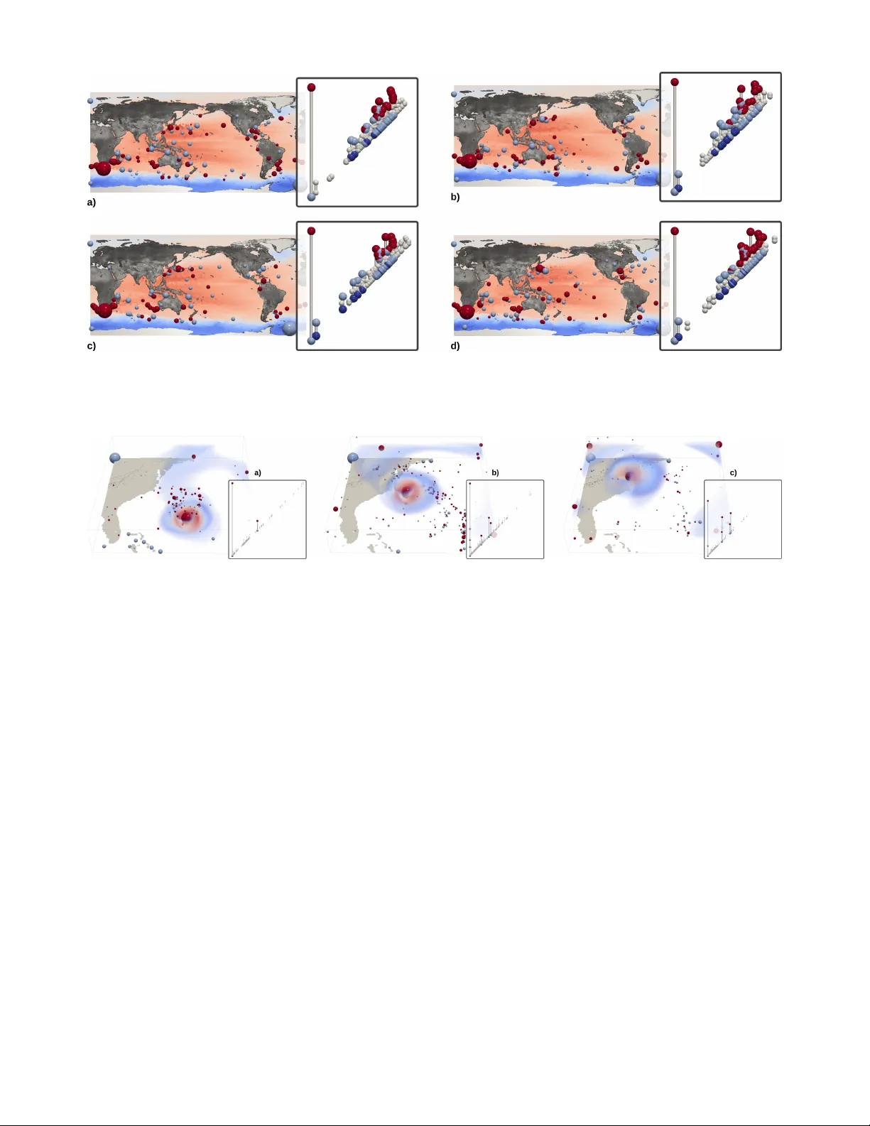
Statistical P arameter Selection for Clustering Persistence Diagrams Max K ontak Simulation and Softwar e T echnology DLR German Aer ospace Center K ¨ oln, Germany max.kontak@dlr .de Jules V idal CNRS LIP6 Sorbonne Universite Paris, France jules.vidal@sorbonne-univ ersite.fr Julien T ierny CNRS LIP6 Sorbonne Universite Paris, France julien.tierny@sorbonne-uni versite.fr Abstract —In urgent decision making applications, ensemble simulations are an important way to determine different outcome scenarios based on currently av ailable data. In this paper , we will analyze the output of ensemble simulations by considering so- called persistence diagrams, which are reduced repr esentations of the original data, motivated by the extraction of topological features. Based on a recently published progr essive algorithm for the clustering of persistence diagrams, we determine the optimal number of clusters, and theref ore the number of significantly different outcome scenarios, by the minimization of established statistical score functions. Furthermore, we present a proof-of- concept prototype implementation of the statistical selection of the number of clusters and provide the results of an experimental study , where this implementation has been applied to real-world ensemble data sets. Index T erms —urgent decision making, ensemble simulation, topological clustering, statistical model selection I . I N T RO D U C T I O N T o support ur gent decision making in the situation of a catastrophic ev ent, ensemble simulations can be used to quan- tify uncertainties and to distinguish different possible outcome scenarios, which may require div erse steps to be taken by a crisis manager . In practice, modern numerical simulations are subject to a v ariety of input parameters, related to the initial conditions of the system under study , as well as the configuration of its en vironment. Gi ven recent adv ances in hardware computational power , engineers and scientists can now densely sample the space of these input parameters, in order to identify the most plausible crisis e volution. The European project VESTEC [1] focuses on building a toolchain combining interactiv e supercomputing, data analysis and visu- alization for the purpose of urgent decision making. Through the VESTEC system, a crisis manager would be able to run an ensemble of numerical simulations and interactiv ely explore the resulting data in order to help the decision making process. Three use cases are to be supported: mosquito-borne diseases, wildfire monitoring, and space weather forecasting. The identification of the possible scenarios can be ac- complished by finding clusters in the simulation results. For instance, for a time-varying wildfire simulation, the outputs of all ensemble simulations for each time step could be clustered This work is partially supported by the European Commission grant H2020- FETHPC-2017 “VESTEC” (ref. 800904). to obtain a time series of clusterings, which can then be further analyzed. In that way , one can determine points in time at which significantly different simulations arise in the ensemble ( e. g. , there is only one fire vs. the fire has split up into multiple parts), which is rele vant for the decision maker , who can compare the different clusters with the behavior of the fire in reality to identify the most plausible crisis ev olution. Unfortunately , the output data sets of large-scale simula- tion codes are often too big to all fit in memory , which creates a need for reduced data representations. These can be provided by topological data analysis [11], [38]. So-called persistence diagrams ha ve been used in many applications before (combustion [7], [19], [26], fluid dynamics [8], [22], material sciences [14], [20], [28], chemistry [6], [17], and astrophysics [34], [36]) to obtain reduced data representations. Recently , an efficient technique has been proposed for clus- tering persistence diagrams instead of the original simulation data [41]. W ith the application of urgent decision making in mind, the algorithm has been designed based on the classical k -means clustering algorithm to incorporate time constraints. Howe ver , the number of clusters k is still a parameter of the approach in [41]. In this work, we will inv estigate so-called information crite- ria , which hav e been de veloped for statistical model selection [9], [24], to determine the optimal number of clusters. W e will present a proof-of-concept prototype implementation for the statistical selection of parameters in topological clustering and perform an experimental study on real-life ensemble data sets. I I . R E L A T E D W O R K Existing techniques for ensemble visualization and analysis typically construct, for each member of the ensemble, some geometrical objects, such as level sets or streamlines, which are used to cluster the original members of the ensemble and to construct aggregated views. Sev eral methods hav e been proposed, such as spaghetti plots [10] for le vel-set variability in weather data ensembles [31], [32], or box-plots for the variability of contours [42] and curves in general [29]. Related to our work, clustering techniques ha ve been used to analyze the main trends in ensembles of streamlines [15] and isocontours [16]. Fa velier et al. [13] introduced an Fig. 1. The persistence diagram (right insets) reduces a data set (top left, bottom left: terrain view) to a 2D point cloud where each off-diagonal point represents a topological featur e . In this diagram, the X and Y axes denote the birth and death of a topological feature, respectively . In these examples, points which stand out from the diagonal represent lar ge features (the two hills, (a) and (b)), while points near the diagonal correspond to noisy features in the data. approach, relying on spectral clustering, to analyze critical point v ariability in ensembles. Lacombe et al. [25] introduced an approach to cluster ensemble members based on their persistence diagrams. More relev ant to our context of urgent decision making, V idal et al. [41] introduced a method for the progressiv e clustering of persistence diagrams, supporting computation time constraints. Ho wev er , this approach, which extends the seminal k-means algorithm [27], is subject to an input parameter, the number of output clusters k , which is often difficult to tune in practice. I I I . B A C K G RO U N D This section presents the technical background of our work. A. T opological Data Analysis T opological Data Analysis is a recent set of techniques [11], [38], which focus on structural data representations. W e re view in the follo wing the main ingredients for the computation of topological signatures of data, for their comparison, and for their clustering. This section contains definitions taken from V idal et al. [41], reproduced here for self-completeness. a) P ersistence diagr ams: The input data is an ensemble of n piecewise linear (PL) scalar fields f : M → R defined on a PL d -manifold M , with d ≤ 3 in our applications. W e note f − 1 −∞ ( w ) = { p ∈ M | f ( p ) < w } the sub-level set of f . When continuously increasing w , the topology of f − 1 −∞ ( w ) can only change at specific locations, called the critical points of f . Critical points are classified according to their index I : 0 for minima, 1 for 1-saddles, d − 1 for ( d − 1) -saddles, and d for maxima. Each topological feature of f − 1 −∞ ( w ) ( e. g. , connected com- ponents, independent cycles, voids) can be associated with a unique pair of critical points ( c, c 0 ) , corresponding to its birth and death . Specifically , the Elder rule [11] states that critical points can be arranged according to this observ ation in a set of pairs, such that each critical point appears in only one pair ( c, c 0 ) such that f ( c ) < f ( c 0 ) and I c = I c 0 − 1 . Intuitiv ely , this rule implies that if two topological features of f − 1 −∞ ( w ) ( e. g. , two connected components) meet at a critical point c 0 , the youngest feature ( i. e. , created last) dies , fa voring the oldest one ( i. e. , created first). Critical point pairs can be visually represented by the persistence diagram , noted D ( f ) , which embeds each pair to a single point in the 2D plane at coordinates  f ( c ) , f ( c 0 )  , which respecti vely correspond to the birth and death of the associated topological feature (Figure 1). The persistence of a pair , noted P ( c, c 0 ) , is then giv en by its height f ( c 0 ) − f ( c ) . It describes the lifetime in the range of the corresponding topological feature. b) W asserstein distance between persistence diagr ams: T o cluster persistence diagrams, a first necessary ingredient is the notion of distance between them. Gi ven two diagrams D ( f ) and D ( g ) , a pointwise distance can be introduced in the 2D birth/death space between two points a = ( x a , y a ) ∈ D ( f ) and b = ( x b , y b ) ∈ D ( g ) by d ( a, b ) =  | x b − x a | 2 + | y b − y a | 2  1 / 2 = k a − b k 2 . (1) By con vention, d ( a, b ) is set to zero if both a and b exactly lie on the diagonal ( x a = y a and x b = y b ). The W asserstein distance between D ( f ) and D ( g ) can then be introduced as W  D ( f ) , D ( g )  = min φ ∈ Φ   X a ∈D ( f ) d  a, φ ( a )  2   1 / 2 , where Φ is the set of all possible assignments φ mapping each point a ∈ D ( f ) to a point b ∈ D ( g ) , or to its projection onto the diagonal, ( x a + y a 2 , x a + y a 2 ) , which denotes the removal of the corresponding feature from the assignment. The W asserstein distance can be computed by solving an op- timal assignment problem, for which efficient approximation algorithms exist [5], [23]. It can often be useful to geometrically lift the W asserstein metric by also taking into account the geometrical layout of critical points [35]. Let ( c, c 0 ) be the critical point pair corresponding to the point a ∈ D ( f ) . Let p λ a = λc 0 + (1 − λ ) c ∈ R d be their linear combination with coef ficient λ ∈ [0 , 1] in M . Our experiments (section V) only deal with extrema, and we set λ to 0 for minima and 1 for maxima (to only consider the extremum’ s location). Then, the geometrically lifted pointwise distance b d ( a, b ) is given as b d ( a, b ) = q (1 − α ) d ( a, b ) 2 + α || p λ a − p λ b || 2 2 . The parameter α ∈ [0 , 1] quantifies the importance given to the geometry of critical points and it must be tuned on a per application basis. c) F r ´ echet mean of persistence diagr ams: Once a dis- tance metric is established between topological signatures, a second ingredient is needed, namely the notion of barycenter , in order to lev erage typical clustering algorithms. Let D be the space of persistence diagrams. The discrete W asserstein barycenter of a set {D ( f 1 ) , D ( f 2 ) , . . . , D ( f n ) } of persistence diagrams can be introduced as the Fr ´ echet mean of the set under the metric W . It is the diagram D ∗ that minimizes its distance to all the diagrams of the set ( i. e. , the minimizer of the so-called Fr ´ echet energy), that is, D ∗ = arg min D∈ D P n i =1 W  D , D ( f i )  2 . The computation of W asserstein barycenters in volv es a computationally demand- ing optimization problem, for which the existence of at least one locally optimum solution has been shown by T urner et al. [40]. Efficient algorithms have been proposed to solve this optimization problem [25], including the progressiv e approach by V idal et al. [41], which can return rele vant approximations of W asserstein barycenters, given some user defined time constraint t max , which is rele vant for our urgent decision making context. d) T opological clustering: Once barycenters between topological signatures can be computed, traditional clustering algorithms, such as the k -means [27], can be revisited to sup- port topological data representations. Based on their efficient and progressive approach for W asserstein barycenters, V idal et al. [41] revisit the k -means algorithm as follows. The k -means is an iterative algorithm, where each Clustering iteration is composed itself of two sub-routines: (i) Assignment and (ii) Update . Initially , k cluster centroids D ∗ j ( j = 1 , . . . , k ) are initialized to k diagrams D ( f i ) from the input set. Then, the Assignment step consists of assigning each diagram D ( f i ) to its closest centroid D ∗ j ( i ) . This requires the computation of the W asserstein distances W , of e very diagram D ( f i ) to all the centroids D ∗ j . Next, the Update step consists of updating each centroid’ s location by placing it at the W asserstein barycenter of its assigned diagrams D ( f i ) . The algorithm continues these Clustering iterations until con ver gence, that is, until the as- signments i 7→ j ( i ) between the diagrams and the k centroids do not e volv e anymore. Since W asserstein barycenters can be approximated under user-defined time constraints with V idal’ s approach [41], the above algorithm also supports time constraints (see [41] for further details). Of course, a larger time constraint will, in general, result in a better clustering of the input set of persistence diagrams. B. Statistical scores The previously described method assumes that the number of clusters k is known a priori . If the number of clusters is not known in advance, so-called information criteria can be used to select a number of clusters a posteriori after the k -means algorithm has been applied for sev eral values of k . In our application, we will use the Akaike Information criterion (AIC, [2], [3]) and the Bayesian information criterion (BIC, [33]), which are based on the minimization of a score function of the form IC( k ) = 2 L ( k ) + p ( k ) , (2) where L ( k ) is the v alue of the log-likelihood function of the clustering result, when k clusters are detremined, and the term p ( k ) penalizes the number of parameters differently for AIC and BIC. The criteria can be interpreted as a way to balance the goodness of fit (represented by the log-likelihood function) and the number of parameters: on the one hand, the goodness of fit is minimal if the number of clusters and the number of data points coincide, but the number of parameters is high in this situation. On the other hand, if the number of clusters is minimal, then the goodness of fit is, generally , very large. The minimum v alue of the information criterion will, consequently , be somewhere inbetween. Under the so-called identical spherical assumption (see [30]), it can be shown (originally , for data from a Euclidean space) that the log-likelihood term has the form L = k X j =1 n j log n j − n log n − n d 2 log(2 π ˆ σ 2 ) − d 2 ( n − k ) , (3) where n j is the number of diagrams mapped to the centroid D ∗ j , n is the total number of diagrams, d is the dimension of D , and ˆ σ is an estimation of the in-cluster variance, for example, ˆ σ 2 = 1 d ( n − k ) n X i =1 W ( D ( f i ) , D ∗ j ( i ) ) 2 . (4) Since the dimension of D cannot be easily determined, we choose a value for d in our prototype implementation such that the information criteria show the expected behavior (ap- proximately conv ex, being monotonically decreasing for small k and monotonically increasing for large k ). The penalty term p in (2) for the AIC is giv en by p AIC ( k ) = 2 k d, whereas for the BIC it is giv en by p BIC ( k , N ) = k d log ( N ) (cf. [12], Sect. 13.3), where the term k d encodes the number of effecti ve parameters of the statistical model, particularly , the d coordinates of the k cluster centers. Note that for a comparison of different clusterings of a fixed data set, p AIC and p BIC do indeed only depend on k , since both the dimension d of the underlying space as well as the number N of samples is constant. I V . P R OT OT Y P E I M P L E M E N TA T I O N This section details the implementation of our prototype. Fig. 2. Clusters automatically identified by our topological clustering approach ( t max : 10 seconds) on the Sea Surface Height data-set. Left to right, top to bottom: pointwise mean of each cluster. Inset diagram: cluster centroid computed by the algorithm of V idal et al. [41] (in the diagrams, the X and Y axes denote the birth and death of the topological features, respectiv ely). Barycenter extrema are scaled in the domain by persistence and colored by critical index (spheres). In this example, the four clusters correspond to the four seasons. Fig. 3. Clusters automatically identified by our topological clustering approach ( t max : 10 seconds) on the Isabel data-set. Left to right: pointwise mean of each cluster . Inset diagram: cluster centroid computed by the interruptible algorithm of V idal et al. [41] (in the diagrams, the X and Y axes denote the birth and death of the topological features, respectively). Barycenter extrema are scaled in the domain by persistence and colored by critical index (spheres). In this example, the three clusters correspond to the three hurricane configurations (from left to right: formation, drift and landfall). A. T opological clustering For each ensemble data set, giv en a user time constraint t max , we systematically run the progressiv e topological clus- tering algorithm of V idal et al. [41] for a range of k v alues (typically , 1 to 10 ). For this, we used the companion C++ implementation provided by V idal et al. [41], av ailable in the T opology T oolKit (TTK) [39]. Since the computation is independent for distinct k values, this step can be trivially parallelized (one k -clustering per process/thread). B. Statistical scores Once the clustering has been performed for dif ferent values of k , the computation of the statistical scores (AIC and BIC) is straight-forward if the W asserstein distances of each persistence diagram to its nearest centroid are extracted from the clustering process. Inserting these distances in (4) results in an estimation of the in-cluster variance, which can then be used in (3) to compute the value of the log-likelihood function. Combined with the computation of the penalty terms p AIC and p BIC , one obtains a value of the statistical score for the given clustering. V . R E S U LT S This section presents experimental results obtained with a C++ implementation. The input persistence diagrams were computed with the algorithm by Gueunet et al. [18], which is av ailable in the T opology T oolKit (TTK) [39]. Our experiments were performed on a variety of simulated and acquired 2D and 3D ensembles, taken from Fa velier et al. [13], follo wing the experimental setup of V idal et al. [41]. The Gaussians ensemble contains 100 2D syn- thetic noisy members, with 3 patterns of Gaussians. The Sea Surface Height ensemble (Figure 2) is composed of 48 observations taken in January , April, July and October 2012 (https://ecco.jpl.nasa.gov/products/all/). Here, the features of interest are the center of eddies, which can be reliably esti- mated with height extrema. Thus, both the diagrams in volving the minima and maxima are considered and independently processed by our algorithms. Finally , the Isabel data set (Figure 3) is a volume ensemble of 12 members, showing key time steps (formation, drift and landfall) in the simulation of the Isabel hurricane [21]. In this example, the eye wall of the hurricane is typically characterized by high wind velocities, 1 2 3 4 5 6 7 8 9 10 1 2 3 4 5 6 7 8 9 10 1 2 3 4 5 6 7 8 9 10 (a) Gaussians ensemble 1 2 3 4 5 6 7 8 9 10 1 2 3 4 5 6 7 8 9 10 1 2 3 4 5 6 7 8 9 10 (b) Sea Surface Height ensemble 1 2 3 4 5 6 7 8 9 10 1 2 3 4 5 6 7 8 9 10 1 2 3 4 5 6 7 8 9 10 (c) Isabel ensemble Fig. 4. V alues of the AIC (solid line) and BIC (dashed line) for k = 1 , . . . , 10 for the three ensemble data sets for t max = 1 s , 10 s , 100 s (left-to-right). The values have been normalized to the value for k = 1 for each diagram. Therefore the Y axes are not labeled. The X axes denote the number of clusters. well captured by velocity maxima. Thus we only consider di- agrams in volving maxima. Unless stated otherwise, all results were obtained by considering the W asserstein metric W based on the original pointwise metric in (1) without geometrical lifting ( i. e. , α = 0 , subsection III-A). In Figure 4, we hav e depicted the values of the statistical score functions for these three data sets for three different values of t max , where the number of clusters is characterized as the minimizer of the score functions. W e hav e marked the number of clusters, determined with the most accurate clus- tering (that is, t max = 100 s ) with a vertical line. W e observe that for the less accurate clusterings ( t max = 1 s , 10 s ), we may obtain either a just slightly different number of clusters (Gaussians ensemble) or a number nearly doubling the optimal number of clusters (Sea Surface Height ensemble). This might seem to be a drawback with regard to the application of urgent decision making, where small values of t max are desirable. Howe ver , in practice, when comparing the identified clusters with the crisis situation in reality to determine the most likely outcome, it is very helpful if the number of clusters is much lower than the number of ensemble simulations. This is still the case both for slightly different numbers of clusters and also for a twice as high number of clusters. Additionally , when determining the number of clusters in time-varying ensemble simulations, as described in the introduction, it is especially interesting if the number of clusters changes at a specific time step. W e expect that these changes will also take place with the less accurate numbers of clusters. Of course, this will be analyzed in more detail in the future, when the presented method will be applied to data sets from the pilot applications used in the VESTEC project [1]. Figure 2 shows our results for the Sea Surface Height ensemble, where our statistical analysis estimates an optimal number of clusters of k = 4 and where the topological cluster- ing [41] automatically identifies four clusters, corresponding to the four seasons: winter , spring, summer , fall (left-to-right, top-to-bottom). As shown in the insets, each season leads to a visually distinct centroid diagram. As discussed by V idal et al. [41], geometrical lifting is particularly important in applications where feature location bears a meaning, such as the Isabel ensemble (Figure 3). For this example, our statistical analysis estimates an optimal number of clusters of k = 3 and the clustering algorithm with geometrical lifting [41] automatically identifies the right clusters, corresponding to the three states of the hurricane (formation, drift and landfall). V I . C O N C L U S I O N Motiv ated by urgent decision making applications, which require the clustering of ensemble simulation outputs for the determination of different crisis scenarios, we proposed a statistical technique to determine the number of clusters based on a recently published progressiv e clustering method for so-called persistence diagrams. W e presented a proof-of- concept prototype implementation, which pro vided meaningful results for real-world ensemble data sets. In our upcoming research, we will incorporate the parameter selection within the clustering approach directly based on this prototype. Us- ing Paravie w Catalyst [4], [37], our approach can easily be integrated into any simulation code. It then allows to carry out in-situ clustering operations on a statistically determined number of clusters at chosen iterations of the simulation, while respecting the time constraints of an urgent decision making situation. Furthermore, in the context of the European project VESTEC [1], we will apply our approach to o t her real-life use cases (wildfire, mosquito-borne diseases, space weather) and, especially , in an in-situ context to allow for an interaction of the decision maker with the ensemble simulations. A C K N O W L E D G M E N T S The authors would like to thank the anonymous revie wers for their thoughtful remarks and suggestions. R E F E R E N C E S [1] VESTEC EU Project. 2018-2021. https://vestec- project.eu. [2] H. Akaike. Information theory and an extension of maximum likelihood principle. In B. Petrov and F . Csaki, eds., Second International Symposium on Information Theory , pp. 267–281, 1973. [3] H. Akaike. A ne w look at the statistical model identification. IEEE T rans. Automat. Contr . , 19:716–723, 1973. [4] U. A yachit, A. Bauer, B. Ge veci, P . O’Leary , K. Moreland, N. Fabian, and J. Mauldin. Para view catalyst: Enabling in situ data analysis and visualization. In Pr oceedings of the F irst W orkshop on In Situ Infrastructur es for Enabling Extreme-Scale Analysis and V isualization , ISA V2015, pp. 25–29. ACM, New Y ork, NY , USA, 2015. [5] D. P . Bertsekas. A new algorithm for the assignment problem. Math. Pr ogram. , 21:152–171, 1981. [6] H. Bhatia, A. G. Gyulassy , V . Lordi, J. E. Pask, V . Pascucci, and P .-T . Bremer . T opoMS: Comprehensiv e topological exploration for molecular and condensed-matter systems. J. Comput. Chem. , 39:936–952, 2018. [7] P . Bremer, G. W eber, J. Tierny , V . Pascucci, M. Day , and J. Bell. Interactiv e exploration and analysis of large-scale simulations using topology-based data segmentation. IEEE T rans. V is. Comput. Gr . , 17:1307–1324, 2011. [8] F . Chen, H. Obermaier , H. Hagen, B. Hamann, J. T ierny , and V . Pascucci. T opology analysis of time-dependent multi-fluid data using the reeb graph. Comput. Aided Geom. D. , 30:557–566, 2013. [9] G. Claeskens and N. Hjort. Model selection and model averaging . Cambridge University Press, 2008. [10] P . Diggle, P . Heagerty , K.-Y . Liang, and S. Zeger . The Analysis of Longitudinal Data . Oxford University Press, 2002. [11] H. Edelsbrunner and J. Harer . Computational T opology: An Intr oduction . American Mathematical Society , 2009. [12] B. Efron and T . Hastie. Computer Age Statistical Infer ence . Cambridge Univ ersity Press, 2016. [13] G. Fa velier , N. Faraj, B. Summa, and J. Tiern y . Persistence Atlas for Critical Point V ariability in Ensembles. IEEE T rans. V is. Comput. Gr . , 25:1152–1162, 2018. [14] G. Favelier , C. Gueunet, and J. Tiern y . V isualizing ensembles of viscous fingers. In IEEE SciV is Contest , 2016. [15] F . Ferstl, K. Brger , and R. W estermann. Streamline variability plots for characterizing the uncertainty in vector field ensembles. IEEE T rans. V is. Comput. Gr . , 22:767–776, 2016. [16] F . Ferstl, M. Kanzler , M. Rautenhaus, and R. W estermann. V isual analysis of spatial variability and global correlations in ensembles of iso-contours. Comput. Graph. F orum , 35:221–230, 2016. [17] D. Guenther, R. Alvarez-Boto, J. Contreras-Garcia, J.-P . Piquemal, and J. Tiern y . Characterizing molecular interactions in chemical systems. IEEE Tr ans. V is. Comput. Gr . , 20:2476–2485, 2014. [18] C. Gueunet, P . Fortin, J. Jomier, and J. Tierny . T ask-based augmented contour trees with fibonacci heaps. IEEE T rans. P arall. Distr . , 30:1887– 1905, 2019. [19] A. Gyulassy , P . Bremer, R. Grout, H. K olla, J. Chen, and V . Pascucci. Stability of dissipation elements: A case study in combustion. Comput. Graph. F orum , 33:51–60, 2014. [20] A. Gyulassy , V . Natarajan, M. Duchaineau, V . Pascucci, E. Bringa, A. Higginbotham, and B. Hamann. T opologically clean distance fields. IEEE Tr ans. V is. Comput. Gr . , 13:1432–1439, 2007. [21] IEEE SciV isContest. Simulation of the Isabel hurricane. http:// sciviscontest- staging.ieee vis.org/2004/data.html, 2004. [22] J. Kasten, J. Reininghaus, I. Hotz, and H. Hege. T wo-dimensional time- dependent vortex regions based on the acceleration magnitude. IEEE T rans. V is. Comput. Gr . , 17:2080–2087, 2011. [23] M. Kerber , D. Morozov , and A. Nigmetov . Geometry helps to compare persistence diagrams. ACM Journal of Experimental Algorithmics , 22, 2016. Article No. 1.4. [24] S. Konishi and G. Kitagawa. Information Criteria and Statistical Modeling . Springer, 2007. [25] T . Lacombe, M. Cuturi, and S. Oudot. Large scale computation of means and clusters for persistence diagrams using optimal transport. In S. Bengio, H. W allach, H. Larochelle, K. Grauman, N. Cesa-Bianchi, and R. Garnett, eds., Advances in Neural Information Pr ocessing Sys- tems 31 (NIPS 2018) , 2018. [26] D. E. Laney , P . Bremer, A. Mascarenhas, P . Miller, and V . Pascucci. Un- derstanding the structure of the turbulent mixing layer in hydrodynamic instabilities. IEEE T rans. V is. Comput. Gr . , 12:1053–1060, 2006. [27] S. Lloyd. Least squares quantization in PCM. IEEE Tr ans. Inform. Theory , 28:129–137, 1982. [28] J. Lukasczyk, G. Aldrich, M. Steptoe, G. Favelier , C. Gueunet, J. Tierny , R. Maciejewski, B. Hamann, and H. Leitte. V iscous fingering: A topological visual analytic approach. Appl Mech. Mater . , 869:9–19, 2017. [29] M. Mirzargar , R. Whitaker, and R. Kirby . Curve boxplot: Generalization of boxplot for ensembles of curves. IEEE Tr ans. V is. Comput. Graph. , 20:2654–2663, 2014. [30] D. Pelleg and A. Moore. X-means: Extending k-means with efficient estimation of the number of clusters. In ICML ’00: Proceedings of the Seventeenth International Confer ence on Machine Learning , pp. 727– 734, 2000. [31] K. Potter, A. W ilson, P . Bremer, D. Williams, C. Doutriaux, V . Pascucci, and C. R. Johnson. Ensemble-V is: A framew ork for the statistical visualization of ensemble data. In 2009 IEEE International Conference on Data Mining W orkshops , 2009. [32] J. Sanyal, S. Zhang, J. Dyer , A. Mercer, P . Amburn, and R. Moorhead. Noodles: A tool for visualization of numerical weather model ensemble uncertainty . IEEE T rans. on V is. Comput. Graph. , 16:1421–1430, 2010. [33] G. Schwarz. Estimating the dimension of a model. Ann. Stat. , 5:461– 464, 1978. [34] N. Shi vashankar , P . Pranav , V . Natarajan, R. v an de W eygaert, E. P . Bos, and S. Rieder . Felix: A topology based framework for visual exploration of cosmic filaments. IEEE T rans. V is. Comput. Gr . , 22:1745–1759, 2016. http://vgl.serc.iisc.ernet.in/felix/index.html. [35] M. Soler, M. Plainchault, B. Conche, and J. Tierny . Lifted W asserstein Matcher for Fast and Robust T opology T racking. In IEEE Symposium on Large Data Analysis and V isualization , 2018. [36] T . Sousbie. The persistent cosmic web and its filamentary structure: Theory and implementations. Mon. Not. R. Astron. Soc. , 414:350–383, 2011. http://www2.iap.fr/users/sousbie/web/html/indexd41d.html. [37] The T opology T oolKit usage tutorial. TTK in-situ with Catalyst. https: //topology- tool- kit.github .io/catalyst.html, 2019. [38] J. Tierny . T opological Data Analysis for Scientific V isualization . Springer , 2018. [39] J. Tiern y , G. Fa velier , J. A. Levine, C. Gueunet, and M. Michaux. The Topology ToolKit. IEEE T rans. V is. Comput. Gr . , 24:832–842, 2017. https://topology- tool- kit.github .io/. [40] K. Turner, Y . Mileyko, S. Mukherjee, and J. Harer. Fr ´ echet Means for Distributions of Persistence Diagrams. Discr ete Comput. Geom. , 52:44– 70, 2014. [41] J. V idal, J. Budin, and J. Tiern y . Progressi ve W asserstein Barycenters of Persistence Diagrams. IEEE T rans. V is. Comput. Gr . , 2019. accepted for publication. [42] R. T . Whitaker, M. Mirzargar , and R. M. Kirby . Contour boxplots: A method for characterizing uncertainty in feature sets from simulation ensembles. IEEE T rans. V is. Comput. Gr . , 19:2713–2722, 2013.