Deep Learning for Prostate Pathology
The current study detects different morphologies related to prostate pathology using deep learning models; these models were evaluated on 2,121 hematoxylin and eosin (H&E) stain histology images captured using bright field microscopy, which spanned a…
Authors: Okyaz Eminaga, Yuri Tolkach, Christian Kunder
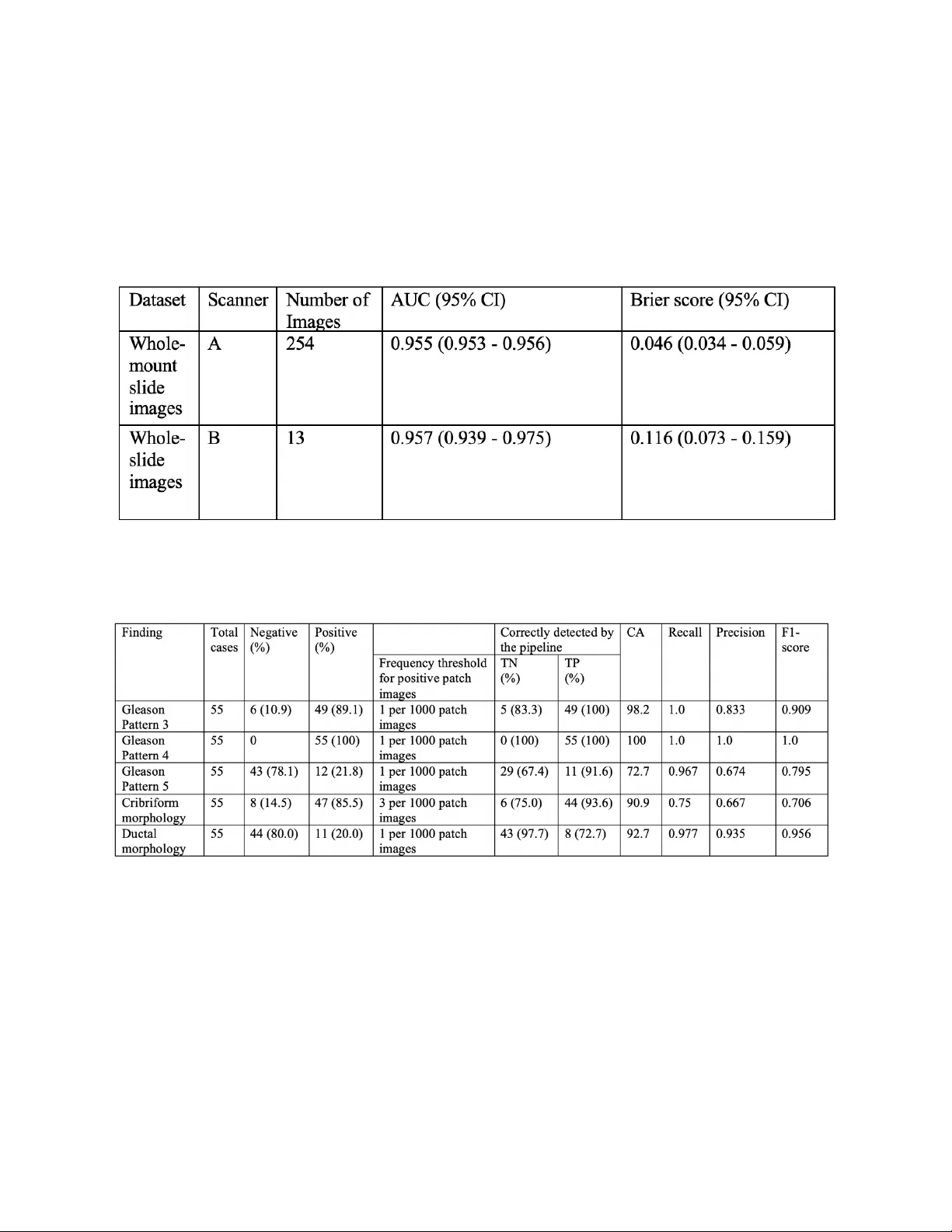
Deep Learning fo r P ro s t a t e Pa t h o l o g y Okyaz Eminaga (1,2 ,3,4 ) , Yuri Tolkach* (5) , Christian Kunder* (6) , Mahmood Abbas* (7) , Ryan Han ( 8) , Rosalie Nolley (2) , Axel Semjonow (9) , Martin Boegemann (9) , Sebastian Huss ( 10 ) , Andreas Loening ( 11 ) , Robert West (6) , Ge offrey Sonn (2) , Richard Fan (2) , Olaf Bettendorf (7 ) , James Brook (2) and Daniel Rubin ( 3,4 ) *Equally contributed. 1) DeepMedicine.ai 2) Dept. of Urology, Stanford University School of Medicine 3) Dept. of Biomedical Data Science, Stanford University School of Medicine 4) Center for Artificial Intelligence in Medicine & Imaging, Stanford Medical School 5) Dept. of Pathology, Bonn University Hospital 6) Dept. of Pathology , Stanford University School of Medicine 7) Institute for Pathology and Cytology, Schuettorf, Germany 8) Dept. of Computer Science, Stanford University 9) Prostate Center, Dept. of Urology, University Hospital Muenster, Germany 10) Dept. of Pathology, Department of Urology, University Hospital Muenster, Germany 11) Dept. of Radiology, Stanford University School of Medicine [ This manuscript is subject to change an d will be removed as soon as officially published by a peer - reviewed journal . T he final version o f the manuscript will be published by a peer - reviewed journal . The manuscrip t includes patented methods . Any use of the method s with out permission is prohibited fo r c ommer cial use .] Corresponding author: Okyaz Eminaga, M.D./Ph.D. Department of Urology, Center for Artificial Intelligence in Medicine & Imaging (AIMI), Laboratory of Quantitative Imaging and Artificial Intelligence (QIAI ) Stanford University School of Medicine 300 Pasteur Drive Stanford CA 94305- 5118 Tel: 650 - 725 - 5544 Fax: 650- 723 - 0765 Email: okyaz.eminaga@stanford.edu Stanford University, Stanford Medical School Abstract The current study detects different morphologies related to prostate pathology using deep learning models; these models were evaluated on 2, 121 hematoxylin and eosin (H&E) stain histology images captured using bright field microscopy, which spanned a variety of image qualities, origins ( whole slide , tissue micro array , whole mou nt , Internet), scanning machines, timestamps, H&E staining protocols, and institutions. For case usage , t hese models were applied for the annotation tasks in clinician-oriented path ology report s for prostatecto my specimens . The true positive rate (TPR) for slides with prostate cancer was 99.7% by a false positive rate of 0. 7 85 % . The F1 - scores of Gleason patterns reported in pathology reports ranged from 0.795 to 1.0 at the case level. TPR was 93.6% for the cribriform mo rphology and 72.6% for the ductal morphology . The correlation between the ground truth and the prediction for the relative tumor volume was 0.987 n. Our models cover the major components of prostate pathology and successfully accomplish the annotation ta sks . Introduction Prostate Cancer (PCa) is the most diagnosed cancer in men and one of the most prevalent cancer- related causes of death 1 . PCa is usually diagnosed via prostate needle biopsy and may result in patients undergoing radical prostatectomy (total removal of the prostate, seminal vesicles and surrounding tissues) upon histological confirmation 2 . Management of patients requires a reliable histopathological evaluation , including an initial determination of tumor extent and other cancer- related metrics (particularly grading). However, the limited human resources and the increase in the workload challenge the pathologists to maintain their evaluation performance during the clinical routine. Moreover, the prostatectomy s pecimens are processed in multiple embeddings (up to 50) and represent one of th e specimens that have th e most ti me-consuming evaluation process in the anatomical pathology. The results from the histopathological evaluation are critical for decision -making and predicting the patient’s out come , mak ing reproducibility and standardization of clinical importance 3 . While t he histopathological evaluations of the prostatectomy specimens for the grading and staging of PCa are b ased on well -established guidelines 4,5 , stan dardizing the pathological evaluation has proven to be a challenge due to factors such as the sub stantial interinstitutional differences i n laboratory techniques and human reliability (int ra - /int erobserver variability) 5,6 . Pathologists are human beings whose mental capacities , visual perception, and responses are intuitively expected to vary at the individual level and are also influenced by socioeconomic conditions. Moreover, t he histopathological evaluation generally represents a visual search and de coding task that depends on t he human attentional capacity. It has been shown that human observers often differ in respon se to the same sensory stimuli for the same task, which explains the intra/inte robserver variation in tumor grading 4,6,7 . Interestingly, ad vance information has been shown to enhances the visual search performance 8 . Moreover, p roviding prior information about the sample or igin and location, in addition to the clinical data, has shown to improve the pathological evaluation 9,10 . Accordingly , we propose that providing prior information about the tumor extension and morpholog y can be helpful to guide a more precise histopathological evaluation. Recent advances in Artificial intelligence (AI) especially in computer vision has demonstrated its potentials for automated cancer detection and the tumor grading from histology images 11 - 17 . Deep learning (DL) is a board fam ily of the machine learning methods within the AI domain . DL is considered as one of the state of the art algorithms in computer vision due to its remarkable perform ance in vision detection and segmentation tasks 18 . Most published works to date utilized publicly available “state- of -the art” neural network architectures like VGG16 19 , Inception V3 20 , ResNet 18 , DenseNet 21 for tumor detection and grading problems . Se veral works have successfully shown the effectiveness of DL models in determining cancer lesions and perform ing tumor grading for PCa 11 - 17 . However, apply ing such DL model architectures to the cancer detection and grading task is hindered by the need for expensive computational resources and the absence of well -annotated development datasets. An ideal DL model for the medical domain would be trainable on a small or mid-size data set using affordable or existing infrastructure. Transfer learning is an approach to train a model on small/midsize datasets by r eus ing the pre - trained weights from a large dataset designed for a general image classification problem (e.g., ImageNet). However, the histology images are domain specific datasets that differ significantl y fro m the dataset for the general image classification problems . Accordingly , optimizing the transfer learning remains challenging for the cancer detection problems from the histology images. Transfer learning further requires a comp licated fine -tuning of the pretrained models like , for example, identifying the right layers to tr ain the layer weights 22,23 . Thus, we cho se to use Ple xusNet, a customized deep l earning architecture , that provides comparable resul ts to “state- of -the-art” models for prostate cancer detection with limited resources 23 . For a real case usage, PlexusNet and other customized convolutional neural network architecture inspired by VGG were used for automated annotation to disentangle the annotation work fr om the pathologist’s tasks. For that p urpose, we utilized a framework based on cMDX© (Clinical Map Document based on XML) for the generation and management of clinician-oriented pathology reports already introduced by Eminaga et al 24 . The cMDX framework has been applied in clinical routine to reporting and analyses of PCa in prostatectomy specimens 25 . In this context, the topo graphical distribution of PCa foci and related pathologic findings can be evaluated using the cMDX documentation system 24,25 . However, our previous work was limited by the dependency on the pathologists who delineated the tumor extension using the cMDX Editor. Additionally, the annotation work and the documentation of Gleason patterns an d pathological morphology (i.e. cribriform and ductal morphology ) for each lesion remained time- consumi ng and are thus often times avoided by the pathologists . Given the restrictions of the previous works, this study will illustrate how AI can improve the existing framework utilized in clinical routine by taking over the annotation tasks and provid e initial information for pathological evaluation. Results Prostate C ancer and related Findings The interobserver annotation agreement between CK and OK/YT was acceptable by an average Cohen -Kappa score of 0.8385 (range: 0.7468 - 0.9284). The detection model for prostate cancer was validated internally and externally on 3 datasets representing the digitalized whole -mount (WM) slide images, the regular whole- slide (WS) images, and TMA. The comparison analyses to baseline methods (e.g. Inception V3 and MobileNet V2) related to prostate cancer detection are already handled by E minaga et al 23 . Although these datasets wer e acquired using d ifferent types of scanners, PCa detection achieved AUC-ROCs range between 0.954 and 0 .9 57 or Brier score range between 0.046 and 0.134 per slide for WM/WS images or at spot level for TMA ( Figure 1 and Table 1 ). AUC -ROC reveals the classification performance at different thresholds ; a higher AUC -ROC indicates a better classification accuracy, where a AUC-ROC of 1 represents the highest accuracy ; t he Brier score is used as a measure of the model "calib ration"; th e lower the brier score , the better the model is calibrated. A c oefficient of determination (R 2 ) of 0.987 was mea sured for the correlation between relative tumor volumes of the ground truth (the tumor annotation made by CK for WM images of each case was considered as ground truth) and the predicted relative tumor volumes in 46 cases ( Supplement Fil e 1) . The paired t-test also showed no significant differences between the relative tumor volumes of the ground truth and the predicted relative tumor volu mes (t-statistic: -0.499; P=0.619). The mean relative tumor volume was 9.95% for the ground truth and 11.0% for the predicted volume; the mean dif ference between both relative volumes was - 1.08 % (95% CI: - 1.44 - 0.72 ). Our model correctly classifi ed the slides in 99% (402/406) of the cases. The positive predictive value (PPV) was 99.2% and the negative predictive value (NPP) was 95.8%. The true positive rate (TPR) was 99.7%, while the false positive rate was 0.7 85 % ( Supplement File 1 ). [Remo ved due to copyright issue] Figure 1 shows the general workflow for the detection part of the current study. For simplicity, we presented the results from prostate cancer and for the pathology features Gleason patt erns 3 and 4 and HGPIN (High - grade intraepitheli al neoplasia). The pathology r eports do not routinely include HGPIN as the clinical benefits of HGPIN are limited on final pathology re ports of prostatectomy specimens. Detai led results are provided i n supplement file 1. The tumor bur den was calculated by identifyi ng the average number of pixels with tumor in rela tion to the pixel siz e on the mask patches gener ated from the annotation data in each data source. w/o: without; w: with; PCA: Prostate cancer ; PPV: Positive predictive value; NPV: negative predictive value ; TPR: true positive rate, TNR: true negative rate; CA: Classification accuracy; AUC: Area under curve of the receiver operati ng characteristic curve , FMI: Fowlkes - Mallows index . * a complete ground truth (annotation ) for the tumor exte nt of the prostate cancer was available f or 46 cases. TCGA: The Cancer Genomics Atlas; Table 1 : The slide - wise a ccuracie s for prostate cancer detection on external datasets calculated on patch images per slide. Table 2 : The accuracies for Gleason pattern de tection, cribriform and ductal mor phology on cases that have who le - mount s ections of the prostate. The frequency thres holds of the finding presence required for reporting at a case level were set to 0.1% for most findings . We tested the model performance for Gleason pattern 3 (GP3) and pattern 4 (GP4) on an external ISUP dataset ( Figure 1 and Table 3 ). Here, the model achieved an AUC of 0.937 and a F1- score of 0.9 for GP3 and 0.83 for GP4. At the case level, GP3 was correctly identified in 97% of cases and all cases with GP4 were detected correctly. The detection model for Gleason pattern 5 (GP5) achieved a F1-score of 0.9 at patch level and TPR of 91.6% at case lev el. Table 3 : The model acc uracies for Gleason patte rn detection on an extern al dataset from ISUP. Each image was evaluated by expert panel members (23 members). This dataset reached a consensus rate of 65% among pathologists. 95% Confidence Interval for uncert ainty measuremen t determined by bootst rapping with 1000 replica tions) The cribriform or ductal morpholo gy was detected with AUCs of 0.928 or 0.870 at the patch level. At the case level, TPR for the detection of cribriform mo rphology was 93.6% with an overall F1- score of 0.706 whereas TPR for the detection of ductal morphology was 72.7% with an overall F1 - sc ore of 0.956. Rea l C ase Usage of Deep Learning Models for clin ician - oriented c MDX report s Figure 2A/B demonstrates the annotation results and illustrates examples of the activation maps for different findings . By visual review ing the cMDX reports of 55 cases fo r correctness of the annotation , we found that th e tumor lesions were correctly detected and annotated for all cas es . However, the prostate cancer detection was irritated by the histology of the ejaculatory ducts and falsely considered a small part of th e ejaculatory ducts as tumor area in 4 cases. The accuracy for tumor detection is provided for each case in Suppleme nt file 1 . The finding list of each lesions were randomly reviewed, and we confirmed that all the finding listed for the lesion were correct. Figure 3 provides an overview of the user-interface for viewing the cMDX reports. An example cMDX file and the viewer tool are provided on GitHub (https://github.com/oeminaga/cmdx_report.git) . The user interface provides information related to the presence of Prostate Cancer, Gleason patterns 3, 4 and 5, the cribriform and ductal morphology , and the relative /a bsolute tumor volume. Similar to the original cMDX report editor, the path ologist can provide the tumor grading according to the Gleason grading system 26 , the tumor stage using the UICC TNM staging system 27 , the extracapsular extension and the surgical margin status. Supplement file 2 provides an example of cMDX file that inclu des repre sentative images of the PCa lesions. By Looking at the file sizes, 55 cMDX report s occupied 36.9 gigabytes whereas the corresponding gigapixel histology images required 1.4 terabytes of storage spaces. [Remo ved due to copyright issue] F igure 2A the slide thumbna il (Grid) was used to def ine a grid to sp lit the his tology image i nto p atches, fro m which the t umor probability was determined for each patch and a heatmap was reconstructed. Th e generation of the heatmap was repeated for other findings and the heatmap f or the prostate cancer wa s used to determ ine the lesion bound ary (AN NO). PC A: Prosta t e Cancer; DA: Ductal mo rphology ; CRI: Cribriform morph ology ; Gleason pattern 3 (GP3), 4 (GP4) or 5. Nerve and/or vessel structures ( NERV/VES); inf lammation (INF) signatures of h igh - grade intraepi thelial neoplasia (HGPIN); Automated annotati on of the lesion (Anno) . [Remo ved due to copyright issue] F igure 2B the activation map for different findings. signatures of high - grade intraepithelial neoplasia (HGPIN) [Remo ved due to copyright issue] F igure 3 : The graphical user interface of the c MDX report v iewer ( A). The user ca n access the or iginal gigapix el histology images if these ima ges are availab le on the local sto rage. By clicking o n the lesion (ma rked with red c olor), a second w indow showi ng the region appears (B). The user can zoom in or out and scrol l through the lesion. The original i nput data were altered for patient’s privacy reasons . Discussion The current study demonstrated th at deep learning models for different histology of prostate pathology are feasible . As real case usage , we demonstrated the feasibility of us ing these models for annotation tasks of the electronic cMDX (clinical map document ) pathology reports as t he original framework for the cMDX pathology reports is already part of the clinical routine in Prostate Center of the University Hospital Muenster for more than a dec ade 24,25 . Our work differs from previous works 11,12,14,28 - 33 in prostate cancer and Gleason pattern detection in many significant ways. First, the current study covered various types of histology images in cluding the whole -mount slide of a prostatectomy slice, the whole-slide image that contains a portion of the prostatectomy slice, a TMA slide, and internet images ( i.e., ISUP images). Second, we utilized histology i mages that cover all anatomical zones of the prostate and the seminal vesicle . We preferred the whole-slide H&E images of prostatectomy specimens over the biopsy samples f or this study for the following reasons. The prostate consists of four major anatomy regions (i.e., peripheral zone, central zone, transition zon e and anterior fibromuscular stroma), where the peripheral zone occupies 70% of the prostat e 34 . Each prostatic zone h as its own hi stological features that distinguish itself from other zones 34 . Usually, the systematic biopsy scheme targets the peripheral zone as the majority of prostate cancer originates from this zone (68%). However, the remaining prostate cancer is located in other zones which are usually not targeted by the syst ematic biopsy scheme at the initial biopsy setting due to the low tumor probability in these zones 35,36 . As the maximum cylindric tissue volume for a 18-gauge biopsy s ide -notch needle with 2.5 cm stroke length is 0.0316 cc 37,38 and the prostate vol ume ranges between 24 and 106 cc 39,40 , a single biopsy core represents a small fraction of the prostate. Thus, the prostate biopsy is not representative due to the heterogeneity of prostate tissue and prostate cancer and is associated with sampling errors 41 . The pathology evaluation of prostatectomy specimens reflects more the real pathological conditions of th e prostate cancer and provide s more apparent pathological evidences (e.g. tumor heterogeneity, tumor volume and tumor extent) than the pathology evaluation of biopsy cores 42 . Further, the current GG system for b iopsy is limited by many challenges associated with sampling errors, high interobserver variations, the biopsy targeting angles and its discrepancy to the final GG in 30-40% cases 4,43 . Thus , the GG system of prostatecto my , if available, is preferred as reference path ology over that of prostate biopsy. For in stance , s tudies evaluating the GG upgrading, a frequent situation i n PCa , are considering t he GG of the prostatectomy specimens as reference or final GG to identify cases whose final GG are upgraded from the biopsy GG 44,45 . Another example is the Epstein criteria for active surveillance that was developed on the basis of the pathology evaluation of prostatectomy specimens 46,47 .In light of this, the generalizability of the deep learning models that were developed based on biopsy samples or TMA for prostate cancer detection or grading remain questionabl e. Third, the current study cover ed different finding families and were evaluated on different d atasets for robustness and performance consistence. The cancer detection accuracies remained stable over different types of histology images and scan ner types. Our findings show that our model based on the PlexusNet architecture 23 performed well in prostate cancer detection and Gleason patterns although it was developed by usin g 12 .7% of the total histology images. The discrepancy in the performance of the HGPIN detection model between the internal vali dation set annotated by YT and the external validation set annotated by CK is due to the inconsistency in the definition of HGPIN lesion as the current inter-observer agreement for HPGIN is 70% according to Iczkowski et al 48 . Fourth, we provided a real case usage of our models by integrating the detection models into the electronic cMDX pathology report. The cMDX pathology report was designed from the urological aspect and includes information relevant for tumor classification (pT) from whole- mounted prostatectomy specimens such as the tumor spatial distribu tions 27 and the presence of Gleason patterns. Using the detection model for prostate cancer facilitated a very accurate estimation of the tumor volume related to the ground truth (R 2 :0.987). One of the challenges of reporting tumor volume is the accurate estimation as it is one of the reasons for controversy in the predictive value of tumor volume or relative tumor volume 49 - 53 . A lt hough no consensus method has emerged for measuring tumor volume, ISUP advocates for technological advances in imaging techniques to reinforce the clinical rationale for incorporating a size-related staging parameter into the pathological reporting of prostate cancers 54 . Finally, we followed the clinical guidelines for pathological evaluation and considered the needs of urologists for histopathological information in the cMDX reports 24 . F ifty- five cases were tested on a single GPU and the models were also trained on a single GPU (Titan V with 11 GB VRAM) and 2 TB PCIe flash memory , where one case required 35+/-6 minutes in average to complete the all finding detections. This duration includes the time cost for input/output access that has impacts on the processing speed. Th us, our models are energy efficient compared to models that require multiple GPUs or expensive GPU cloud solutions for training. We believe that energy- /cost - effective AI-based solutions will re ceive more acceptance in healthcare as a recent survey showed that the majority of U.S. public (69%) advocates the need for prioritizing the reduction of healthcare cost by the U.S. government 55 . Deep learning has now facilitated the automation of the time- con suming annotation procedure for the tumor extent and helped to shorten the considerable documentation duration required for the manual delineation of the tumor extent 25 . Given that there is no standard validation set for prostate cancer to compare with results from other studies, we explicitly avoided any comparison with previous stu d ies . In our opinion, performing a model comparison is artificial and challenging because the model optimization depends on the developers and the data preparation. Additionally, there is no standard configuration for hyperparameters or augmentations for the existing models for prostate cancer and related findi ngs. The condi tion of the input data (e.g. the magnification level and patch size), configurations of hyperparameters (e.g. batch size) or augmentations (e.g. the degree of rotation) lead to different performance despite having the same model ar chitecture 14,23,56,57 . Moreover, there are so many deep learning architecture and many trimmed versions of “state- of -art” models making a reasonable model comparison difficult for one research team to cover the all existing d eep le arning models 14,28,33,58 - 60 . Therefore, we advocate providing detailed information related to the model architecture, the hardware, the hyperparameter and augmentation configuration, and conducting the model evaluation on a standard validation set to achieve a reasonable model comparison. To support the standardized performance reportin g for prostate cancer detection and related finding, the image file list, the annotation data for TCGA images will be availabl e f or non -commercial research. The current study inherits some limitations that warrant mention. First, this study has a retrospective character and therefore encompasses the limitations of a retrospective study . Although we implemented a quality control procedure for the blurriness and brightness of histology images, the protective measurement may have failed to i dentify poor-quality images that may have impacted the model performance. Thus, a periodi c quality control of histology images should be made prior to fe eding the framework with histology images. There is a need to adapt the deployment of DL models to the existing i nfrastructure and resources. Further, the definition of the thresholds for cancer detection varies according to the application as the evaluation conditions for biopsy cores differs from for the evaluation conditions of prostatectomy specimens. Other limitations include the high expense and maintenance costs of the infrastructure to digitalize histology slides that continue to restrict t he wide -spread usage of digital pathology. We believe that this issue can be resolved by having more competitors i n this field to lower the costs to benefit small and midsize healthcare services. A potential limitation of this study is that many pathologists were involved in the annotation procedures. However, such cond itions actually mimic the clinical routine and the classification performance for PCA, GP3 and GP4 detection were comparable between different datasets with histology images annotated by diff erent path ologists. We didn ’t p erform any comparison to the human reade rs as such comparisons are artificial and do es n’t represent the clinical routine ; The clinical routine includes a close communication between differe nt cli nical discipline s and physicians through many channels ( e. g. hospital information systems, tumor boards, consulting et c.. ) and it is well - known that pr ior kn owledge about the clinical information enhances the pathology evaluation 9,10 . Another limitation is th at the classification accuracy for Gleason pattern 5 (GP5) was moderate due to the low number and size of the lesions with GP5 as Gleason pattern 5 of our cases are tertiary Gleason patterns and the patients with GG 9-10 are often not amenable to su rgical intervention and instead receiving hormonal deprivation and radiation therapy 61,62 . However , the detection model for GP5 has a space for accuracy improve ment and we aim to recruit more cases with Gleason pattern 5 to enhance the accuracy of the GP5 detection model over the time. Finally, we focused o nly on major findings related to prostate pathology and did n’t consider all aspects of prostate pathology. However, the purpose of th e curren t study is to show that DL is feasible to determine di fferent morphologies of prostate pathology and we do plan to expand the coverage to benign hyperplasia and intraductal prostate can cer based on the existing highly curated datasets. Our future work will focus on integrating the DL into the cMDX framework and conduct research evaluating the benefits of applying DL trained on prostatectomy specimens for biopsy pathology. Conclusion The current study introduces deep learning models for different histology of prostate patho logy deployable for cMDX pathology report generator; it has high accuracies for cancer detection and the detection of related findings. Material and Methods This study used prospectively collected whole-slide di agnostic histology images (TCGA-PRAD) from TC GA ( The C ancer Genome Atlas) and Stanford University in accordance with the privacy regulations and the Helsinki declaration. The study was approved by the IRB (IRB- 4641 8 ). The histology images were stained with Hematoxylin and Eosin staining (H&E) and acquired using an Aperio Digital Pathology Slide Scanner -Scanner type A- from Leica Biosystem (Wetzlar, Germany). The TCGA images were scanned at a 40x objective zoom, whereas the Stanford images were scanned at a 20x o bjective zoom. These images were stored in SVS format. Our cohort consisted of 449 H&E images from TCGA ; 466 whole -mount H&E images from 65 cases who underwent radical prostatectomy were also considered. Additionally, we included 125 whol e- slide images representing the index lesions in 125 cases from the historic McNeal dataset that were scanned at 40x objective zooming level using a slide scanner from Philips (Amsterdam, Netherland) – Scanner B. A tissue micro array (TMA) from 339 prostatectomy specimens with 932 spots from prostate cancer index lesions and 197 spots with normal tissues was stained wi th H&E and scanned u sing the Ariol microscope system manufactured by Leica -Scanner C- (Wetzlar, Germany). For ty-two spot images from a second TMA that have, in addition to normal tissue and prostate cancer, prostatic intraepithelial neoplasia was also included in our study. Finally, 220 H&E histology images from the International Society of Urological Pathology (ISUP ) reference library images were included (Internet, Unknown scanner vendor). In total, we collected 2,431 H&E i mages that spanned a variety of image q ualit ies , origins (WS, TMA, WM, Internet), scanni ng machines, timestamps, H&E staining protocols, and institu tions. All histology images were capture using the bright field microscopy. For real case u sage, we appl ied the existing cMDX framework for generating pathology reports for prostatectomy s pecimens and includ ed the automated annotation of prostate cancer and related findin g. A detailed description of cMDX framework can be obtained from Eminaga et al 24 . Cohort for Prostate Cancer Detecti on The development set was randomly selected and consisted of 250 histology images from TCGA (55% of TCGA images) and 60 whole-mount histology images from 10 S tanford cases (12% of Stanford WM images). The main reason of including 10 cases from Stanford is the high tumor burden of TCGA images (Mean pixel number with tumor i n percentage: 45+/- 4%), which does not cover all aspects of histological structures of the prostate (e.g., ejaculatory duct, d ifferent forms of the benign hyperplasia, epithelial tissues from central zones, urethra). Therefore, we selected these images from Stanford that have tumor burdens below 10% of the prostate and exhibit different prostatic anatomic structures. The development set was then randomly split into a training set (80%), and a test set for internal validation (20%). The validation set for model training was generated by randomly selecting 10% of patch images from each case of the test set. All images were annotated for tumor lesions by experienced board-certified pathologists (CK, YT, MA and RW) and a urologist (O E ) who all have significant experience in research related to the pathology of prostate cancer and its associated findings. The prostate cancer lesions of the whole -mount (WM) images were annotated by CK. The annotation of the tumor lesions on the regular whole-slide (WS) images from TCGA-PRAD and McNeal’s dataset was made by OE and confirmed by MA for the correctness of the annotation. The tissue micro arrays (TMA) for prostate cancer was already created according to the tumor status. The spots with tumors were obtained from lesions in prostatectomy specimens that were identified by many pathologists during the cl inical routine. After creating the TMA, the tumor status of each TMA spot was evaluated and confirmed by R W. For external validation, we utilized three datasets with different data origins. The first validation set consisted of 254 whole-mount H&E images from serially sectioned prostatectomy specimens. The second validation set had 13 whole-slice H&E images f rom the McNeal dataset. The third external data set with H&E images came from the Stanford Tissue Microarray (TMA) Database with prostate cancer (n= 1,129) and was applied for evaluating detection performa nce. These histology spot images (Size: 1,024x1,024 pixels) were stained with H&E, captured at 20x objective magnification level. We clipped the middle region of the spot image which contains the tissue with rele vant findings by 512x512 pixels an d applied the repeated fi ll effect with the cl ipped image for a new image with a size of 1,024x1,024 pixels, which was then resized to 512x512 pixels for each H&E image. To evaluate the inter-observer annotation agreement, 6 whole -mount images from Stanford were independently annotated for the prostate cancer lesions by YT (OE refined the marked l esion bou ndaries ) and KC and the inter-observer agreement was estimated by Cohen Kappa after setting a grid with tiles of 512 x512 pixels for each image. Cohort for Findings related to Prostate Cancer Sixty-four H&E whole slice images were randomly selected from the development set including 58 images from Stanford and 6 images from TCGA dataset. YT annotated the regions of interests (ROI) covering all findings listed in Supplement file 3 and the annotation contours of ROI were refined by OE . Gleason grading was made in accordance with ISUP guidelines from 2016 63 . T he regions of interest were tiled by 512x512 pixels , and the resulting patch images were split after the stratification by case into the development sets (70%, n=44) and internal validation sets (30%, n=20). From the development set, we generated a training set with 90% of the development set and the remaining lesions were assigned to the model validation set. In order to account for class imbalance (arbitrary defined by a ratio of 8:1 for the majority and minority classes) when it occurred, we applied the oversampling of the minority class to increase the frequency of the patch images from the minority class. Supplement file 3 provides information regarding the findings that have the imbalance class problems and the app lied factor to oversample the minority class for solving this problem. It is worth noting that the internal validation set (test set) consists cases that have a detailed morphology annotation as given in Su pplement file 1 and 3 . Further, we visually checked subsets of patch images from the internal validation set for the presence of Gleason patterns 3, 4, and 5 to ensure that patch images represent the correspond ing findings ( Supplement file 1 ). We didn ’t consider th e Gle ason pattern s less than 3 in our stu dy as these patterns are no longer utilized in clinical routine due to the lack of the c linical implication 4 . Gleason grading plays an important role in clinical decision making and we wanted to ensure that our models for Gleason pattern 3 and 4 provide results comparable to those of experts. Therefore, we utilized the International Society of Urological Pathology (ISUP) reference library images for Gleason grading, which were graded by a majority voting of a panel of 23 expert members of ISUP, to externally validate our models fo r Gleason pattern 3 and 4 64 . Here, we considered 220 H&E images (Size: 2048x2048 pixels, captured at 20x magnification level) havi ng either 4+4 or 3+3 Gleason score for our evaluation to limit the risk of the inaccurate evaluation and finding uncertainty in each patch image and to increase the likelihood of the presence of a single finding in each patch image . Further, we wanted to ensure that our models can correctly detect the Gleason patterns from ISUP histology images as these images are considered as Gold standard and used for education purposes. We were unable to evaluate Gleason pattern 5, given that there are 6 images with Gleason pattern 5 concurrent with Gleason pattern 4. High-grade Intraprostatic intraepithelial neoplasia (HGPIN), the most presumed precursor of prostate cancer 65,66 , is opti onally reported in the pathology reports 67 . So, i t was important to validate th e model for HGPIN d etection by using an external validation set from a TMA containing HGPIN (20 of 42 spots). Spots with HGPIN were labelled by a single experienced uro-pathologists (CK), whereas the development set with HGPIN lesions from WM images was annotated by YT and the marked boundaries of the lesions were refined by OE . Since the validation sets were acquired usin g scanners other than those used for the development set, we optimized the brightness of the patch images by multiplying with a scanner factor th at may range between 0.01 and 1. The determination of the scanner factor is based on the brute force approach, which finds the best scanner factor by determining the best ROC performance of the model on 5 positive and 5 negative patch images from the new dataset with no need to re-tr ain the model for new slide images captured by scanners other than we used for the development set. The screening for the best scanner factor was made at two steps by the sequential increasing of the scanner factor initially by 0.1 and then by 0.01 in a cl osed range containing the best factor from the initial screening. Generatio n and Labelling of Patch Images To define the coordinate grid for patch image generation, the smallest level of the SVS whol e - slide image was converted to grayscale. Then, the tissue region was masked by thresholding at the mean gray value of the gray intensity. To determine the coordinates of each patch image, the default patch size (512x512 pixels) was rescaled after dividing by scale factors for height and width. These scale factors were determined by calculating the ratio of the dimension of the whole -slide image at 10x to the image dimension of the highest level. Patches were generated with an overlap ratio o f 0.2. Patch es not covered by the masked tissue region were excluded in order to remove background images from the dataset. Finally, the grid for t he patch images was upscaled after multiplying by the scale factors. All histological images were tiled by 512x512 pixels (330x330 µm) at a 10x magnification level based on the grid coordinates. For labelling patch images used for training and validation, the ground truth was considered as a binary mask generated b ased on the annotation data that covered all findings relevant for the current study in each s lide image. We developed a custom patch image generator that generates these masks for model training and evaluation by conducting a key search for required findings in the annotation data. Each finding was annotated on th e slide images independently from other findings. The definition of the negative set depends on the target finding as given in Supplemen t file 1 . The patch mask is extracted at the same l ocation of the corresponding patch image. The percentage of positive pixels to the total image size was estimated to label each patch image according to the binary classification . A patch image is positive if the number of positive pixels meets or exceeds a threshold of 20%. By determi ni ng the threshold, the effec t of potential errors associated with the annotation procedure was taken into account, especially in the edges of the annotated areas as the edge areas are more prone to annotation errors and false-positive conditions than other parts of the annotated region. We also estimated the threshold by building an analogy to the risk of prostate cancer ranges between 15-25% by a threshold of 3- 4 ng/mL for the serum level of prostate-specific antigen, where urologists usually consider an active measurement by the given risk for prostate cancer 68 . Color Intensity Optimization for Hematoxylin Eosin for aged whol e- slide H&E images A long storage period of H&E slides from McNeal datasets > 10 years and aging processes caused paled H&E staining of these slides. Specially, the nuclei staining is affected the most by aging. In order to reconstruct the color intensity, we deve loped an algorithm specific for the color i ntensity correction of H&E McNeal images inspired by Macenko’s approach 69 . Before feeding the patch images for any prediction procedures, we converted the RGB color space of the patch images into the optical density (OD) space for red, green and blue channels. Then, we restricted the OD ranges between 0.5 and 0.95 and excluded extreme values of OD. After that, we calculated the covariance matrix of a single patch image first by combining the color channels with itself and then with each other and calculated the mean covariance matrix from all channel combinations. Finally, the eigen vector was calculated using the mean covariance matrix and equalized to the stain vector. The determination of the stain vect or occur s once for each WS H&E image using the first patch image. The obtained stain vector is applied to optimize the color intensity of nuclei for all patch images originated from McNeal’s whole-slide H&E images by multiplying the stain vector with the O D for ea ch patch image. Finally, the OD matrices for red and green and blue channels were converted back to the matrices with the RGB color space. The patch image is corrected by merging the converted matrices and the original RGB patch image. An example s howing a patch image before and after applying the H&E color optimization is provided in S upplement file 1 . Deep Learning models for Cancer Detection and Detection of other findings r elevant for pathology report Supplement file 3 provides information related to t he cohort constitution, the model architecture, and the hyperparameters applied for each finding considered in our screening report. Additional information about the CNN architecture of each model can also be obtained from supplement file 1 . Most model s we re trained using the optimization algorithm Adaptive Moment Estimation (i.e., ADAM) instead of Stochastic Gradient Descent 70 . The g radient Noise was applied for models to improve the model learning as the noise induced by the stochastic process aids generalization by reducing overfitting 71 . The maximum number of training epochs was set to eit her to 50 or 20 and an early stopping algorithm was used to stop training after five consecutive epochs with not improvement in t he classification accuracy . The b atch size was defined as 16 . Relevant findings other than cancer were delineated on the randomly selected 62 H&E images from Stanford and TCGA by OE under supervision of MA and YT. The relevant findings and their proportions in the development and test sets for each model are listed in Supplement file 1 and 3 . After that, the regions of i nterests were extracted and tiled by 512x512 pixels and applying an overlap rate of 0.5. These tiled images were split into a training set , validation set , and test set. CL AHE (Contrast Limited Adaptive histogram equalization) was applied for some models i n order to optimize the image contrast an d all pixel values were normalized by 1/255. We applied class weighting, oversampling, and image augmentation of rare findings to reduce the class imbalance effect and increase the presence probability of these scarce findings in the batch sequence during the model training. The image augmentation included rotation, horizontal and vertical flips, image shearing, and zooming and brightness manipulation. Additionally, we applied random RGB channel shifting and random modification of the image quality by changing the JPEG compression rate for certain findings. Planimetric Cancer volume estimation The prostate volume was calculated after formalin fixation by weighing the prostate specimen without the seminal vesicles. For the purpose of our study, the prostate weight in grams was considered roughly equivalent to its volume in cubic centimeters (cm 3 ); the tumor/entire gland ratio i s then used to calculate the volume o f the tumor in cm 3 . A correction factor for tissu e shrinkage after formalin fixation was not considered. The computational tumor volume estimate was performed on the basis of the volumetric calculation. Every tumor focus in each slice is estimated by counting the pixels affected by PCa. The cancer area i s then divided by the slice area occupied by the prostatic slice and then added to calculate the relative cancer volume . Finally, the total relative cancer volume is multipl ied with the prostate volume to calculate the cancer volume in cm 3 . Study Cohort fo r the accuracy eva luation of path ology screening reports Slides of sequential whole-mount slices from 55 cases that underwent prostatectomy were scanned at a 20x objective zoom and then fed into the cMDX framework. The whole -mount H &E hi sto logy slides were digitalized for all slices of the prostate from prost atectomy specimens in each case. The Gleason patterns were extracted from pathology reports of these cases using a natural language process and the keyword search. These extracted findings were further checked for correctness by manually reviewing the pathology reports and then compared with the reported Gleason pattern in the automated pathology reports . The pathology reports and H&E slide images were evaluated for the presence of ductal and cribriform morphol ogy at the case level ( OE evaluated the pathology reports and shared anonymized histology images with MA for evaluation). The relative tumor volume was compared between the ground truth annotation made by CK and the relative tumor volume calculated by the cMDX pathology report . Evaluation metrics The c lassification performance of the final test set for pathological findings was evalu ated once using classification accuracy, precision, recall, F-measure (F1 score) , Area Under of the Receiver Operating Characteristics curve (AUC -ROC), and Brier score. F1 - score is the harmonic mean between of the precision and recall applied for the measurement of the classifi cation performance and imbalanced classi fication problems. The Fowlkes -Mallows index (FMI) is defined as the geometric mean between of the precision and recall and genera lly used for the similarity me asurement between two groups. The Brier score measures the accuracy of probabilistic predictions for binary outcome and can also be used as “calibration” measurement of the prediction model . We evaluated the classification performance slide- wise, spot -wise, and patch-wise for prostate cancer, and case-wise, patch- wise or spot -wise for Gleason patterns 3 and 4. The presence of Gleason pattern 5 was evaluated at the case level. The classification performance of the framework for ductal and cribriform morphology was evaluated at the case level as well. Given that vessel and nerves are widely spread inside the prostate, we considered only the internal validation. The coefficient of the regression score determined the correlation of relative tumor volumes between the ground truth and the cMDX framework at case level . The pair-wise student t-test was applied to identify the significance of variation between the groun d truth and the cMDX/PlexusNet-based tumor extent detection for relative tumor volume. The reported p-value is two-sided and statistical significance was assumed as P ≤ 0.05. Our analyses were based on Python 3.6 (Python Software Foundation, Wilmington, DE) or R 3.5. 1 (R Foundation for Statistical Computing , Vienna, Austr ia ) and appli ed the Keras library which is built -on the TensorFlow framework, to develop the models. All ana lyses were performed on a GPU machine with 32 -core AMD processor with 128 GB RAM (Advanced Micro Devices, Santa Clara, CA), 2 TB PCIe flash memory, 5 TB SDD Hard disks, and a single NVIDIA Titan V GPU with 12 GB VRAM. Acknowledgment PlexusNet and the derivate digital markers for survival and genomic alteration are patented. Reference 1. Jemal, A., Siegel, R., Xu, J. & Ward, E. Cancer statistics, 2010. CA Cancer J Clin 60 , 277 - 300 (2010). 2. Abdollah, F. , et al. A competing-risks analysis of survival after alternative treatment modalities for prostate cancer patients: 1988- 2006. European urology 59 , 88 - 95 (2011). 3. Epstein, J.I., Srigley, J., Grignon, D. & Humphrey, P. Recommendations for the reporting of prostate carcinoma: Association of Directors of Anatomic and Surgical Pathology. American journal of clinical pathology 129 , 24 - 30 (2008). 4. Egevad, L., Delahunt, B., Srigley, J.R. & Samaratunga, H. International Society of Urol ogical Pathology (ISUP) grading of prostate cancer - An ISUP consensus on contemporary grading. APMIS 124 , 433 - 435 (2016). 5. Fine, S.W. , et al. A contemporary update on pathology reporting for prostate cancer: biopsy and radical prostatectomy specimens. E ur Urol 62 , 20 - 39 (2012). 6. Elmore, J.G. , et al. Pathologists’ diagnosis of invasive melanoma and melanocytic proliferations: observer accuracy and reproducibility study. bmj 357 , j2813 (2017). 7. Shen, S. & Ma, W.J. Variable precision in visual perceptio n. Psychological review 126 , 89 (2019). 8. Madden, D.J. Adult age differences in the attentional capacity demands of visual search. Cognitive Development 1 , 335 - 363 (1986). 9. Martins, T.R. , et al. Influence of Prior Knowledge of Human Papillomavirus Status on the Performance of Cytology Screening. Am J Clin Pathol 149 , 316 - 323 (2018). 10. Nakhleh, R.E., Gephardt, G. & Zarbo, R.J. Necessity of clinical information in surgical pathology. Arch Pathol Lab Med 123 , 615 - 619 (1999). 11. Arvaniti, E. , et al. Automated Gleason grading of prostate cancer tissue microarrays via deep learning. Sci Rep 8 , 12054 (2018). 12. Arvaniti, E. , et al. Author Correction: Automated Gleason grading of prostate cancer tissue microarrays via deep learning. Sci Rep 9 , 7668 (2019). 13 . Li, J. , et al. An EM -based semi-supervised deep learning approach for semantic segmentation of histopathological images from radical prostatectomies. Comput Med Imaging Graph 69 , 125 - 133 (2018). 14. Campanella, G. , et al. Clinical-grade computational pathology using weakly supervised deep learning on whole slide images. Nature Medicine (2019). 15. Nagpal, K. , et al. Development and validation of a deep learning algorithm for improving Gleason scoring of prostate cancer. npj Digital Medicine 2 , 48 (2019). 16. Li, J. , et al. An attention-based multi-resolution model for prostate whole slide imageclassification and localization. arXiv preprint arXiv:1905.1 3208 (2019). 17. Lawson, P., Schupbach, J., Fasy, B.T. & Sheppard, J.W. Persistent homology for the automatic classification of prostate cancer aggressiveness in histopathology images. in Medical Imaging 2019: Digital Pathology , Vol. 10956 109560G (International Society for Optics and Photonics, 2019). 18. He, K., Zhang, X., Ren, S. & Sun, J. Deep residual learning for image recognition. in Proceedings of the IEEE conference on computer vision and pattern recognition 770 - 778 (2016). 19. Simonyan, K. & Zisserman, A. Very deep convolutional networks for large-scale image recognition. (2014). 20. Szegedy, C., Vanhoucke, V., Ioffe, S., Shlens, J. & Wojna, Z. Rethinking the inception architecture for computer vision. in Proceedings of the IEEE conference on computer vision and pattern recognition 2818 - 2826 (2016). 21. Iandola, F. , et al. Densenet: Implementing efficient convnet descriptor pyramids. arXiv preprint arXiv:1404.1869 (2014). 22. Yosinski, J., Clune, J., Bengio, Y. & Lipso n, H. How transferable are features in deep neural networks? in Advances in neural information processing systems 3320 - 3328 (2014). 23. Eminaga, O. , et al. Plexus Convolutional Neural Network (PlexusNet): A novel neural network architecture for histologic image analysis. (2019). 24. Eminaga, O. , et al. CMDX(c)-based single source information system for simplified quality management and clinical research in prostate cancer. BMC Med Inform Decis Mak 12 , 141 (2012). 25. Eminaga, O. , et al. Clinical map document based on XML (cMDX): document architecture with mapping feature for reporting and analysing prostate cancer in radical prostatectomy specimens. BMC Med Inform Decis Mak 10 , 71 (2010). 26. Gleason, D.F. & Mellinger, G.T. Prediction of prognosis for prostatic adenocarcinoma by combined histological grading and clinical staging. J Urol 111 , 58 - 64 (1974). 27. Brierley, J.D., Gospodarowicz, M.K. & Wittekind, C. TNM Classification of Malignant Tumours , (Wiley, 2016). 28. Lucas, M. , et al. Deep learning for automatic Gleason pattern classification for grade group determination of prostate biopsies. Virchows Arch (2019). 29. Achi, H.E. , et al. Automated Diagnosis of Lymphoma with Digital Pathology Images Using Deep Learning. Ann Cli n Lab Sci 49 , 153 - 160 (2019). 30. Fischer, W., Moudgalya, S.S., Cohn, J.D., Nguyen, N.T.T. & Kenyon, G.T. Sparse coding of pathology slides compared to transfer learning with deep neural networks. BMC Bioinformatics 19 , 489 (2018). 31. Jiang, Y., Chen, L., Zhang, H. & Xiao, X. Breast cancer histopathological image classification using convolutional neural networks with small SE-ResNet module. PLoS One 14 , e0214587 (2019). 32. Nagpal, K. , et al. Development and validation of a deep learning algorithm for imp roving Gleason scoring of prostate cancer. NPJ Digit Med 2 , 48 (2019). 33. Litjens, G. , et al. Deep learning as a tool for increased accuracy and efficiency of histopathological diagnosis. Sci Rep 6 , 26286 (2016). 34. McNeal, J.E. The zonal anatomy of the prostate. Prostate 2 , 35 - 49 (1981). 35. McNeal, J.E., Redwine, E.A., Freiha, F.S. & Stamey, T.A. Zonal distribution of prostatic adenocarcinoma. Correlation with histologic pattern and direction of spread. Am J Surg Pathol 12 , 897 - 906 (1988). 36. Rouviere, O. , et al. Use of prostate systematic and targeted biopsy on the basis of multiparametric MRI in biopsy-naive patients (MRI-FIRST): a prospective, multicentre, paired diagnostic study. Lancet Oncol 20 , 100 - 109 (2019). 37. Bostwick, D.G. Evaluating prostate needle biopsy: therapeutic and prognostic importance. CA Cancer J Clin 47 , 297 - 319 (1997). 38. Kanao, K. , et al. Impact of a novel biopsy instrument with a 25- mm side -notch needle on the detection of prostate cancer in transrectal biopsy. Int J Urol 25 , 746 - 751 (2018). 39. Berges, R. & Oelke, M. Age-stratified normal values for prostate volume, PSA, maximum urinary flow rate, IPSS, and other LUTS/BPH indicators in the German male community- dwelling population aged 50 years or older. World J Urol 29 , 171 -1 78 (2011). 40. Pinsky, P.F. , et al. Prostate volume and prostate-specific antigen levels in men enrolled in a large screening trial. Urology 68 , 352 - 356 (2006). 41. Bjurlin, M.A. & Taneja, S.S. Standards for prostate biopsy. Curr Opin Urol 24 , 155 - 161 (201 4). 42. Elgamal, A.A. , et al. Impalpable invisible stage T1c prostate cancer: characteristics and clinical relevance in 100 radical prostatectomy specimens -- a different view. J Urol 157 , 244 - 250 (1997). 43. Epstein, J.I., Feng, Z., Trock, B.J. & Pierorazio, P.M. Upgrading and downgrading of prostate cancer from biopsy to radical prostatectomy: incidence and predictive factors using the modified Gleason grading system and factoring in tertiary grades. Eur Urol 61 , 1019 - 1024 (2012). 44. De Nunzio, C. , et al. The new Epstein gleason score classification significantly reduces upgrading in prostate cancer patients. Eur J Surg Oncol 44 , 835 - 839 (2018). 45. Epstein, J.I. , et al. A Contemporary Prostate Cancer Grading System: A Validated Alternative to the Gleason Score. Eur Urol 69 , 428 - 435 (2016). 46. Ross, H.M. , et al. Do adenocarcinomas of the prostate with Gleason score (GS)
Original Paper
Loading high-quality paper...
Comments & Academic Discussion
Loading comments...
Leave a Comment