Single Image BRDF Parameter Estimation with a Conditional Adversarial Network

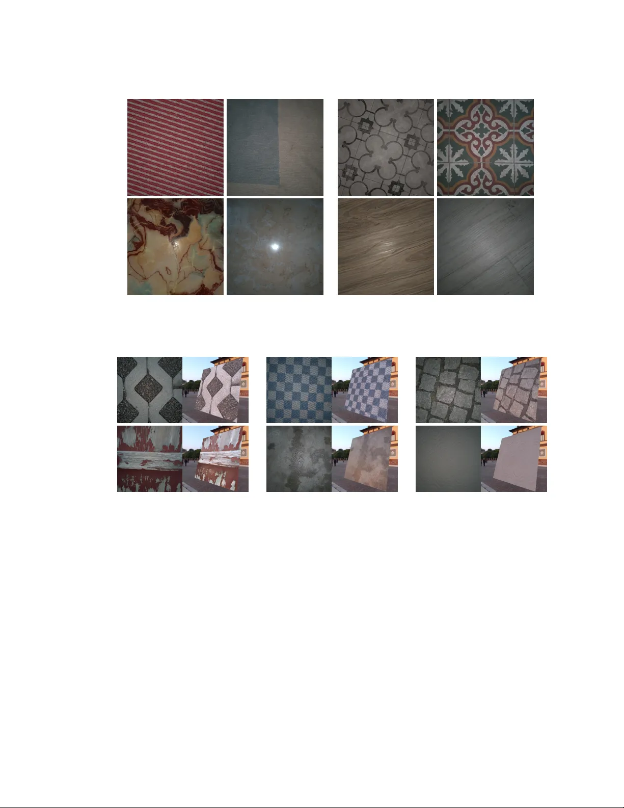
Single Image BRDF Parameter Estimation with a Conditional Adversarial Network MARK BOSS, University of Tübingen HENDRIK P .A. LENSCH, University of Tübingen Fig. 1. For r eal world surfaces our deep neural network predicts spatially-varying BRDF parameters which allow for r ealistic relighting. The prediction is created from a single flash photograph in a casual capture process (le most image). A selection of materials and the accompanying input photographs (upper le) are shown to the right. The 3D-Model is created by Allegorithmic and is available at: https://share.allegorithmic.com/libraries/2887 . Creating plausible surfaces is an essential comp onent in achieving a high degree of realism in rendering. T o relieve artists, who create these surfaces in a time-consuming, manual process, automated retrieval of the spatially-varying Bidirectional Reectance Distribution Function (SVBRDF) from a single mobile phone image is desirable. By leveraging a deep neural network, this casual capturing method can be achieved. The trained network can estimate per pixel normal, base color , metallic and roughness parameters from the Disney BRDF [Burley 2012]. The input image is taken with a mobile phone lit by the camera ash. The network is trained to compensate for environment lighting and thus learned to reduce artifacts introduced by other light sources. These losses contain a multi-scale discriminator with an additional perceptual loss, a rendering loss using a dierentiable render er, and a parameter loss. Besides the local precision, this loss formulation generates material texture maps which are globally more consistent. The network is set up as a generator network trained in an adversarial fashion to ensure that only plausible maps ar e produced. The estimate d parameters not only reproduce the material faithfully in rendering but capture the style of hand-authored materials due to the more global loss terms compared to previous works without r equiring additional post-processing. Both the resolution and the quality is improved. 1 INTRODUCTION With the advance of processing power and improv ements in rendering algorithms, movies and video games approach photorealism. Rendering algorithms recreate the b ehavior of light realistically on the highly detaile d 3D models of characters and scenes. For a high lev el of realism, the correct reectance b ehavior of surfaces is critical. Realistic materials are often captur e d using photogrammetry or with a Bidirectional T exturing Function (BTF) measur ement device. Capturing materials at this quality lev el is often unfeasible b ecause of budget or time constraints as either the capture process is time-consuming or the expenses to develop or acquire a measurement device is high. The other Authors’ addr esses: Mark Boss, University of Tübingen; Hendrik P.A. Lensch, University of Tübingen. 2 Mark Boss and Hendrik P.A. Lensch approach is that artists manually recreate these materials in software suites such as Allegorithmic Substance Designer [Allegorithmic 2018]. However , achieving realistic, manually authored results is a time-consuming process. Ideally , artists want to capture materials quickly with a low-cost device such as a mobile phone . W e propose a method to generate high-quality spatially-varying Bidirectional Reectance Distribution Function (SVBRDF) parameters from low-cost devices with a single, predominantly camera ash lit photograph of a planar surface. T o further aid the artists the reconstructed BRDF parameters should not only recreate the captured material but should imitate human-author e d materials. Reconstructing a BRDF fr om a single view and lighting position is highly ill-posed, and thus the main concern is to estimate BRDF parameters which mainly fulll the human-authored material appearance. W e introduce several loss terms to guide the estimation of isotropic SVBRDF parameters to enforce the human-authored style and thus solv e the ambiguity of this task. The result is parameters for the popular Cook- T orrance model [Cook and T orrance 1982] with the metallic parameter taken from the Disney BRDF [Burley 2012]. W e estimate eight parameters per pixel from a single image input: diuse color (3 channels), normal (3 channels), roughness (1 channel) and metallic (1 channel). Compared to previous work which requires additional post-processing [Li et al . 2018a] or added a priori knowledge [Deschaintre et al . 2018] to reduce artifacts from harsh spe cular reections, our method reduces these artifacts through our novel loss formulation. Fig. 2 visualizes se veral of these problems. This loss formulation forces the generator to learn how to reduce these artifacts, which results in an overall improv e d prediction. The key contributions of this work Input Diuse Specular Normal Roughness Ours Ours Fig. 2. Showcase of several current problems in single shot BRDF estimation. W e compare the prediction of our method to a previous method [Deschaintre et al . 2018]. Notice the artifact by the harsh specular camera f lash of the top material in the diuse and roughness map of the previous method, which is not or hardly visible in our result. In the boom example, the previous method did not remove secondary illumination. For example, the diuse and roughness parameter map displays the light fall o and the secondary illumination in the top right corner . W e remove these artifacts in our prediction (boom). Single Image BRDF Parameter Estimation with a Conditional Adversarial Netw ork 3 are: • W e introduce a Generative Adversarial Netw ork (GAN) architecture with multi-scale discriminators to reduce artifacts from specular highlights. The loss fo cuses more on global structure consistency , and the resulting parameter maps incorporate the human-authored appearance more closely compar e d to previous w orks. This method proofs that a perceptually based loss is helpful in BRDF parameter estimation. • An increase in the SVBRDF parameter map r esolution of a factor of four results in greater detail compared to previous work. Detail is an essential aspect of high-quality BRDFs. • A large proce durally generated BRDF training dataset rendered under varying environment illumination to capture realistic recording scenarios with a mobile phone. The dataset contains 40544 materials with three times dierent environment illumination. 2 RELA TED WORK The concept of capturing BRDFs with an extremely sparse measurement fr om a single image is an active area of research. Several methods address the ill-posedness of the problem. Optimization-based Planar Surface BRDF Estimation. Aittala et al . [2015] use the property that materials ar e often stationary in an optimization approach to t a single tile of an image to other tiles. The result is an SVBRDF from a small low-resolution ar ea of the material. In a follow-up work, Aittala et al . [2018] rene the tile-base d optimization approach by using a pre-trained neural network as a perceptual loss in the optimization and additionally add a dierentiable renderer in the optimization. Deep Neural Network Based Planar Surface BRDF Estimation. Li et al . [2017] are the rst, who explore the possibility of using Convolutional Neural Networks (CNN) for BRDF estimation fr om single input images. The result is spatially- varying information about the diuse and normal parameters and homogene ous parameters for the roughness and specular information. Recently , Li et al . [2018a] and Deschaintre et al . [2018] proposed new network architectures to improve the prediction quality . Both methods introduced a rendering loss where the parameters are evaluated with a dierentiable renderer to provide the network with additional information ab out other lighting conditions. T o further improve the result Li et al . [2018a] added a classication network, which pr ovides additional information about the rough material category to b e used in the decoding step of an enco der-decoder network. They further use a post-processing step based on Conditional Random Fields to enhance the quality of each parameter map. Deschaintre et al . [2018] introduce a global feature track which extracts mean feature vectors by po oling in each encoding and decoding step. They then add these feature vectors to the encoder-decoder network to extract non-local information to aid reducing specular artifacts from the harsh ashlight of the captured surfaces. BRDF Estimation of 3D Objects. Another novel topic is the joint estimation of shape and appearance of 3D objects in a single photograph. For this complex task, the authors need to estimate illumination, shape, and material, which all interact with each other generating complex ambiguities. Recently , two methods tackle this issue. Nam et al . [2018] use several unstructured ash-lit photographs of an object. An optimization approach starts with an initial point cloud estimation using Structure from Motion (SfM) and continues with detailed surface normals and the appearance. The process then uses the lower ambiguity from the now known reectance properties to rene the geometry . Li et al . [2018b] estimate appearance, shape, and illumination from a single predominately ash lit photograph. T o achieve this, they use a deep neural network to learn all tasks jointly . In a rst step, they estimate an initial result for albedo, 4 Mark Boss and Hendrik P.A. Lensch normal, roughness, depth and the environment map represented by spherical harmonics. They then pass the result to a dierentiable renderer which r enders the direct light and environment map approximation. A global light approximation using a pre-trained network adds the contribution of the rst three light b ounces and the image is used to calculate the loss against the input image. T o further improve the resulting parameters they use two additional cascaded networks, which rene the parameters iteratively . Style Transfer and Perceptual Losses. Lastly , the work on image-to-image translation is an important area, as BRDF estimation from a single image can be seen as a style transformation, i.e let@tokene onedotfrom an illuminated surface to its reectance parameters. One of the rst general frameworks for these tasks is proposed by Isola et al . [2017], which can handle a wide variety of translations. They base it on a Generative Adversarial Network ( GAN) architecture . Recently , perceptual losses gained traction in tasks like super resolution and style transfer and surpassed state of the art using pre-trained networks for extraction of features and matching these features fr om prediction to ground truth [Dosovitskiy and Brox 2016; Gatys et al. 2016; Johnson et al. 2016; Sajjadi et al. 2017; W ang et al. 2018]. 3 MA TERIAL REPRESENTA TION T o supp ort artists in material creation, our framew ork estimates parameters for a popular BRDF model often used in modern games such as Unity 1 or the Unreal Engine 2 : the Cook T orrance model with the metallic term introduced by Burley in the Disney BRDF [Burley 2012]. The BRDF is described as: f r = k s + k d . This model consists of the specular lobe k s and the diuse lobe k d . The specular lobe of the Co ok T orrance mo del is dened as: k s = D ( α , ω i , ω o , n ) F ( ω i , ω o ) G ( α , ω i , ω o , n ) 4 ( ω o · n )( n · ω i ) , (1) where D is the normal distribution function, F is the Fresnel term, G is the geometric attenuation factor , α is the roughness parameter , n is the surface normal, and ω i , ω o being the incoming and outgoing direction. For the diuse lobe k d the Disney term is used [Burley 2012]. The GGX normal distribution function drives the microfacet model. As the metallic term only requires a single color map, the base color , the specular and diuse color ne eds to be extracted with the help of the metallic map. Here , an assumption is made. For non-metallic surfaces, the specular color is assumed to be 0 . 04 . This means a 4% base reectance. The diuse color d can then be calculated using d = b ( 1 − m ) and the specular color s using s = 0 . 04 ( 1 − m ) + bm , with b being the base color and m being the metallic value. A metallic value of 1 means metallic and 0 means non-metallic. The base color map needs to b e transformed from sRGB to linear color space for this operation. One large advantage of using this model is that fewer parameters need to be estimated. For the base color and metallic case, only four parameters are required while for specular and diuse color six parameters are to be predicted. 4 NETWORK ARCHITECT URE AND LOSS FORMULA TION Achieving a high prediction resolution and at the same time plausible BRDF parameters, which capture the look and feel of human-authored materials, several challenges need to be addressed. Common loss terms such as a loss against the ground truth parameters or a rendering loss [Aittala et al . 2018; Deschaintre et al . 2018; Li et al . 2018a,b; Nam et al . 2018] provide a reliable per-pixel based training signal. Due to this locality , even with the advanced rendering loss using a dierentiable renderer , the BRDF is often not reliably estimate d 1 https://unity3d.com 2 https://unrealengine.com Single Image BRDF Parameter Estimation with a Conditional Adversarial Netw ork 5 L p L r differen tiable renderer differen tiable renderer Generator G I P fak e P real differen t illuminations differen t illuminations feature loss L f adv. loss L a Discriminator D 1 Discriminator D 1 I , P fak e I , P real feature loss L f adv. loss L a Discriminator D 2 Discriminator D 2 half-res. I , P fak e half-res. I , P real Fig. 3. Conditional generative adversarial network with rendering and multi-scale discriminator loss. The generator network and its input I as well as the output P fake are highlighted in green. The content loss compares the generated parameters P fake and the ground truth parameters P real as well as their respective render e d loss images. Here, L p calculates the MAE loss on the parameter images and the rendering loss L r on the rendered parameters using a dierentiable renderer . The discriminators D 1 and D 2 with their inputs and loss terms ar e highlighte d in purple. The loss terms include an adversarial L a and feature loss L f . It is worth noting that D 2 receives the same input as D 1 but in half the resolution. under every viewing and lighting direction. T o capture plausible parameters matching the style of human-author e d materials for the entire textur e an ade quate style loss is required, which is dened on larger areas than the common per-pixel losses. W e pr opose a GAN ar chite cture with two discriminators to learn the style of human-authored materials. Based on PatchGAN [Isola et al . 2017] the rst discriminator ( D 1 ) receives the input in full resolution, whereas the second discriminator ( D 2 ) receives the input in half resolution. This way the rst discriminator D 1 is responsible for detecting ne details and the second D 2 for larger features. An overview of this structure is visualized in Figure 3. W e sum up the losses from both scales. Importantly , the discriminators conditionally perform their fake or ground-truth prediction given the input photo I and the BRDF parameter P . Thus, the discriminator learns whether the parameters are plausible for a given input photograph and not if the parameters are fr om the material training corpus. Note that during the inference , the prediction of BRDF parameters from an unseen image is purely based on the generator . The loss terms serve the primar y purpose of training the parameters of the generator taking care of all the mentioned concepts. As the U-Net [Ronneb erger et al . 2015] tends to become unstable at higher resolutions the generator architecture is based on the generator of Johnson et al . [2016]. The structure of this network and the two discriminators are described in greater detail in Section 4.3. 4.1 Loss Formulation Overall, our formulation combines three losses: 6 Mark Boss and Hendrik P.A. Lensch • The adversarial loss ensures that the output parameters are in general b ehave similar to other BRDF parameters in the data set. This is achieved in conditional generative adversarial training while tting the predicted parameters to the input image. • The feature loss stabilizes the training procedure by minimizing the distance of high-level featur es b etween ground truth and predictions in the discriminator network. • The content loss is based on a parameter loss and a rendering loss . The parameter loss evaluates the predicted parameter maps directly against the ground truth to provide additional information about ambiguous features in the input image. As there exist ambiguities, the rendering loss enforces plausible material parameter predictions when evaluated against the ground truth under dierent illumination conditions in the image domain rather than in the parameter domain. These loss terms are then combined to a total loss L t for the discriminator and generator . Content Loss. The content loss is a sum of two dierent losses. The rst one is the parameter loss L p . Here, the generated BRDF parameters from the generator are compared to the ground truth parameters. For every parameter map except the surface normals the Mean- Absolute-Error (MAE): ℓ 1 ( A , B ) = 1 n Í n i = 1 | A i − B i | is used„ where A and B are the parameter maps with their n elements. The ℓ 1 loss is preferred over of the Mean-Squared-Error (MSE) loss, as it tends to produce sharper details in the predictions [Zhao et al . 2017]. Intuitively , the MSE loss tends to punish larger errors more than smaller ones, but details are mor e likely visible in small value changes. The linear b ehavior of the MAE loss enforces these small details. As the normal map encodes a normalized vector pointing into the direction of the surface normal, a dierent error metric is used. The angular distance is comparable to the MAE loss in its linear behavior . It is element-wise dened as ℓ ∢ ( a , b ) = cos − 1 ( a · b ) π , (2) with · b eing the dot product between two normalized vectors a , b from given normal maps. T o capture the eect of dierent parameters maps under various illumination conditions, a dierentiable render er produces ten re-renderings with randomly sampled viewing and lighting dir e ctions from the upper hemisphere given the ground truth and the generate d parameter maps. Five of these random light and view positions are chosen such that the y contain a specular highlight by mirroring one randomly sampled direction on a random surface point. The rendering loss L r captures various eects, e.g let@tokeneone dot, by changing the light color randomly metallic reections are explored. T o suppress the large value range in the re-renderings with point light sources, the re-renderings x are monotonously transformed by log ( 1 + x ) . Instead of concentrating only on the error in the sp ecular highlights, this step emphasizes the inuence of all parameters. The MAE loss function is use d to calculate the dierence in the re-renderings yielding L r . Adversarial Loss. An adversarial loss is utilized to enforce parameter map pr e dictions which are indistinguishable from those in the training set. Stability in GAN training is often a problem. Empirical evidence suggests that the LSGAN loss by Mao et al . [2017] improves stability compar e d to the classical cross-entropy based GAN loss [Goodfellow et al . 2014]. The LSGAN loss is dened as: min D L a ( D ) = 1 2 E x ∼ p data ( x ) [( D ( x ) − 1 ) 2 ] + 1 2 E z ∼ p z ( z ) [ D ( G ( z )) 2 ] . (3) Single Image BRDF Parameter Estimation with a Conditional Adversarial Netw ork 7 The term E x ∼ p data ( x ) [( D ( x ) − 1 ) 2 ] forces the discriminator to classify real samples x as 1 and E z ∼ p z ( z ) [ D ( G ( z )) 2 ] ensures fake samples G ( z ) being classied as 0 by the discriminator . In min G L a ( G ) = 1 2 E z ∼ p z ( z ) [ D ( G ( z )) − 1 ) 2 ] (4) the generator on the other hand tries to generate samples G ( z ) which fool the discriminator into classifying them as 1 , eventually synthesizing realistic parameter maps fr om input images z . The discriminator input is a combination of the parameter map and one illuminated image of the material. This way , the conditional adversarial approach learns whether the predicted BRDF parameters are matching the input image rather than just focusing on some features in the parameter set. Feature Matching Loss. The structure of the discriminator acts to some extent as an encoder on these samples, i.e let@tokene onedotit is focusing on and extracting the most important features in the samples. T o further improve the adversarial loss L a an additional feature matching loss between the rst four lay ers from each of the two discriminators D 1 , D 2 is calculated. More specically , the dierence in the feature outputs of each of these layers between the real classication D ( s , p ) and the fake classication D ( s , G ( s )) are calculated. Here, s is dened as the input rendered image, p as the ground truth parameters and G ( s ) as the generate d fake parameters. The loss is then calculated as: L f = 1 S S Õ k = 1 1 L L Õ i = 1 1 N [ D i k ( s , p ) − D i k ( s , G ( s ))] 2 , (5) where S is the number of discriminator scales, L is the number of layers which are compared and N is the number of outputs in each layer . T otal Loss. For the generator , the total loss functions consist of the content loss, feature matching, and adversarial loss. It is calculated as: min G L t ( G ) = 1 4 (L a ( G ) + L f + L p + L r ) . (6) The nal discriminator loss is a combination of the adversarial loss and the feature matching loss min D L t ( D ) = L a ( D ) + λ L f (7) with λ = 0 . 01 . 4.2 Ablation Study Map Proposed −L r % worse −L p % worse −L f % worse −L a % worse Diuse 0.059 0.066 -11.74 0.066 -11.83 0.064 -8.16 0.066 -11.75 Specular 0.047 0.052 -10.93 0.052 -12.64 0.050 -7.14 0.052 -12.41 Normal 0.094 0.101 -7.44 0.095 -1.24 0.099 -4.90 0.104 -10.21 Roughness 0.111 0.117 -5.99 0.119 -7.27 0.120 -8.44 0.114 -3.17 T able 1. Mean error over the test dataset of 7175 samples for various disabled loss terms. Each term is important. The proposed loss consists of several independent loss terms. T o showcase that each loss term provides a signicant contribution towards the nal results, we disable the rendering, parameter , discriminator , and feature loss individually and train the network with the same architecture and training duration described in Se ction 4.4. The trained networks 8 Mark Boss and Hendrik P.A. Lensch Base color Normal Roughness Metallic GT Proposed - L r - L p - L a - L f Fig. 4. Ablation study . A sample of the dataset demonstrates the importance of each loss term. Compared to the ground truth (GT), the proposed loss (second row) matches v er y well. Each disabled loss term degrades the prediction quality . are then used to predict every one of the 7175 samples in the test dataset. In T able 1 the mean degradation in quality over the whole test dataset is sho wn. As seen, every loss term improves the prediction quality . This inuence on the quality is displayed in Figur e 4. Espe cially the contribution of the adv ersarial loss L a is signicant. This is visible in the reconstruction of the ne detail in the metallic map as well as in the lacking detail in the normal map . The parameter and rendering loss help to reduce specular artifacts which ar e visible in the especially visible in the metallic map. O verall the loss term with the highest inuence on prediction quality is the adversarial loss, which suggests that the introduction of an error metric which is not dened on a per-pixel basis is essential in the BRDF estimation quality . This is counter intuitive compared to pr evious tasks like super-resolution ( c.f let@tokene onedot[Johnson et al . 2016; Sajjadi et al . 2017]), where the perceptual based losses achieve higher perceptual quality but worse scores w .r .tlet@tokeneonedotto MSE or PSNR. Howev er , this task is dierent from super-resolution and can be considered a form of style transfer . The large receptive area of the adversarial loss r e duces the chance to run into local minima compared to only leveraging p er-pixel information. Single Image BRDF Parameter Estimation with a Conditional Adversarial Netw ork 9 4.3 Network Architecture The generator architecture is based on Johnson et al . [2016]. How ever , we use pre-activation residual blocks [He et al . 2016]. The discriminator architecture follows the PatchGAN discriminator from Isola et al . [2017]. Here, both discriminators D 1 and D 2 (see Figure 3) use the same architecture, but dierent input resolution. Each discriminator is producing a dier ently sized output. Each output denotes whether the patch is believed to be from a real or fake sample. During training, for each 512 × 512 px input, the D 1 output is a 32 × 32 map and for D 2 a 16 × 16 map. Hence, each entry from the prediction map has a receptive eld of 16 × 16 px or 32 × 32 px area regarding the input image , respe ctively . The detailed network architecture is described in the naming convention used by Johnson et al. [2016]. Generator . c7s1-k 7x7 Convolution-ReLU with k lters and stride of 1. dk denotes 3x3 Convolution-InstanceNorm- ReLU layer with k lters and stride of 2. Rk denotes a pre-activation residual blo ck with k lters. uk denotes a 3x3 Transposed Conv olution with k lters and InstanceNorm with the ReLU activation is used. T o further reduce artifacts at the borders a reection padding is used in every layer of the generator network, except the downscaling d and upscaling layers u : c7s1-64, d128, d256, d512, R512, R512, R512, R512, R512, R512, R512, R512, R512, u256, u128, u64, c7s1-8 . Discriminator . cn-k denotes a 4x4 Convolution-LeakyReLU with a stride of 2 and k lters. ck denotes a 4x4 Convolution-InstanceNorm-LeakyReLU with a stride of 2 and k lters. cns1-k denotes a 4x4 Convolution-LeakyReLU with a stride of 1 and k lters. The LeakyReLU uses a slope of 0.2. Both discriminators use the identical architecture: cn-64, c128, c256, c512, cns1-1 . 4.4 Training The network is traine d for 1.000.000 iterations with a batch size of 8 on four Nvidia 1080 Ti GP Us. The network is trained for 200 epochs with 5000 steps per epoch. The Adam optimizer [Kingma and Ba 2014] is used with β 1 = 0 . 5 and β 2 = 0 . 999 . For the rst 100 ep ochs, the learning rate is set to 2e − 4 and afterward linearly decreased to 0 . The network architecture, including the rendering loss, is implemented in T ensorFlow . 5 D A TASET The dataset is generated with Allegorithmic Substance software and the Substance Share dataset [Allegorithmic 2018]. Community members can upload own procedural materials and rate the uploaded materials. By leveraging the rating system, 175 of the highest rated materials are gathered. From these materials, the list of adjustable parameters is collected. Depending on the number of adjustable parameters up to 100 permutations are generated per material. Each output is generated with all parameters being randomly drawn from a normal distribution with µ being the default value, and σ is set to sample the whole specied value range for the parameter . This ensures that the materials are generated with plausible parameters. The materials are then exported to 2048x2048 pixel parameter maps. These are randomly cropped, rotated and scaled to 512 × 512 pixel resolution seven times. An 80:20 split into training and test data is applied on the Substance les before permutation and post-processing. Overall, this leaves 40544 samples for training and 7175 samples for test. 10 Mark Boss and Hendrik P.A. Lensch Fig. 5. Realistic Dataset. The pairs of similar materials of the synthetic dataset (le) and the real-world (right) indicates that the synthetic set contains realistically looking materials. Samples are visualized in sRGB. Fig. 6. Several real-world photographs with their re-rendered predictions. In each pair the le side is the input f lash photograph and on the right is the re-rendered prediction illuminated by an environment map in sunset. In Figure 5 several real-world and dataset samples are compared. A s seen, the rendered samples from the dataset are hard to distinguish from the real-world ones whenn applying the following processing steps, demonstrating the quality of the synthetic data set: For the input, each material is r endered three times with a randomly r otated High D ynamic Range (HDR) environment map from a pool of 20 outdoor and indoor maps taken from HDRI Haven [Zaal 2018]. The test dataset is only rendered once from a pool of 6 environment maps. The rendering is done in Mitsuba [Jakob 2018] with 196 samples per pixel. The HDR output of the Mitsuba renderer is converted to Low Dynamic Range (LDR) with an auto exposure algorithm. This algorithm calculates an exposure scalar for the photograph. The exact algorithm is outlined in the Appendix A. No Single Image BRDF Parameter Estimation with a Conditional Adversarial Netw ork 11 Input Base color Normal Roughness Metallic Re-rendered Fig. 7. Recovered SVBRDF parameters of specular materials from real-world f lash photographs (le). The sp ecular behavior of each material is captured well. Especially the middle example showcases the high degr e e of detail in the estimation. Here, the dierence in the roughness between the slightly frozen sno w and the grass and dirt is resolved well. The boom example demonstrates that additional light sources from the environment ar e successfully removed. additional tone mapping is applied, and the images are left in linear color space. This step is taken to match raw mobile phone images exported to a linear color space. 6 EV ALU A TION The evaluation is performed b oth on real-world photographs demonstrating the capability to operate on non-synthetic data, and on synthetic data with known ground truth to quantify the error of the estimation. T o match real-world conditions the test set is rendered with a randomly rotated environment map, var ying ash strengths and color temperatures. It is then passed to the auto exposure algorithm (see appendix) and thus converted to LDR. The test dataset is used in this setup, and thus we can compare our proposed method against [2018] and [2017]. 6.1 Real-world P hotographs T wo mobile phones, a Google Pixel 2 and a Samsung Galaxy S9, are used to capture r eal-world data. The images are captured in RA W to minimize post-processing by the mobile phone . The mobile phone is held parallel to the surface with a distance of approximately 50cm, and a camera ash is required for the capture. With this setup, 282 casual photographs of surfaces are captured. The RA W images are then exported in linear color space and cropped with a 1:1 aspect ratio with the camera ash being roughly at the center . Our network is capable of extracting high-quality parameter maps for various surfaces even with multiple mixed materials. In Figure 1 various estimated materials are rendered on a comple x model. The corresponding input image is shown in the upper left corner . As seen the reectance behavior is estimated realistically and matches the input material well. In Figure 7 several challenging surfaces are highlighted. Especially the detail in the reconstructed parameters are noteworthy . For example in the second row , the 12 Mark Boss and Hendrik P.A. Lensch ne surface normal and base color detail for the sno w and the dierent roughness for the snow and grass patches is dicult to predict. The rst r ow highlights that the harsh specular reection of the camera ash is removed successfully and no artifacts are visible in the parameters. The prediction results in a believable surface for the metal plate. The last row highlights the importance of training with envir onment lit renderings. In the input image, an additional light source is visible in the bottom left. Howev er , in the reconstruction, this highlight is removed fully , because the network learned that these light sources are not a reasonable feature of the material. V arious other materials are evaluated in Figure 6. Here, the input image is on the left of each pair and the rendered predictions on the right. Every material realistically reproduces the behavior of each surface. A dditional materials and a vide o showing comparisons under novel viewing and lighting conditions ar e available in the supplementar y . 6.2 Comparison D i f f u se Sp e cu l a r N o r ma l R o u g h n e ss BR D F Pa r a m e t e r 0 . 0 0 . 1 0 . 2 0 . 3 0 . 4 0 . 5 0 . 6 R MSE M e t h o d D e sch a i n t r e e t a l . O u r s O u r s d o w n sca l e d Fig. 8. Comparison to the work of Deschaintre et al . [2018] on our 7175 test materials. As our approach predicts at higher resolution, we compare our results against 512 × 512 px resolution ground truth images and additionally downscale our results with the ground truth to 256 × 256 px resolution to match the resolution used in Deschaintre et al . [2018]. This way parameters with a high degree of fine detail like the normal map can be compared similarly . Our approach is trained to cope with natural illumination besides the f lash light, and this is also true for the test set. Therefore on can note the significantly more precise estimation of the diuse and the roughness channel in our framework. T o correctly quantify the error made by the estimation, the test dataset is used. This dataset, consisting of 7175 materials, is rendered with previously unseen environment maps. Be cause the ground truth parameter is known in this case, the error can be calculated. Additionally , we can compare our method against the method of Deschaintre et al . [2018]. Deschaintre et al let@tokeneonedottrained their method on a similar dataset generated from mostly the same Substance materials from Substance Share ( c.f let@tokeneone dot[Deschaintre et al . 2018]). Additonally , b oth methods use the Cook- T orrance BRDF mo del, but the parametrization is slightly dierent. In section 3 the extraction of the specular and diuse albedo color from the basecolor and metallic parameters is e xplaine d. It is noteworthy that the method of Deschaintre et al let@tokeneonedotonly trained on 256 × 256 px resolution images. Less detail needs to be Single Image BRDF Parameter Estimation with a Conditional Adversarial Netw ork 13 reconstructed by their method. Our method, on the other hand, provides a 512 × 512 pixel resolution output. As Li et al . [2017] try to solve a dierent problem, the estimation from BRDF parameters from only passive illumination, and additionally only estimate spatially-varying diuse and surface normal parameters, we only show results fr om then in a visual comparison (see Fig. 11 and 12). In Figure 8 we compare both methods on the test dataset. Deschaintre et al . [2018] and our approach receive the input in their r espective native resolution. Our method shows better performance in full resolution by a large margin in nearly every parameter except the surface normal. This is due to the ne detail being hardly visible in the render e d image. By scaling our result to 256 × 256 px and comparing against ground truth parameters in the same resolution, our method now achieves even better performance in every parameter . This is shown in Figure 8 as the method ’Ours downscaled’ . This experiment only shows that their approach is not robust to environmental illumination, while the y achieve much better results on their own test data which only contains the ash light. Visually this can be seen in Figur e 11 and 12. In Figure 11 a non-metallic material with a harsh se condary illumination is shown. Our method removes the secondary highlight successfully while a strong artifact from the specular highlight is visible in the roughness parameter in the prediction of Deschaintre et al . [2018] and Li et al . [2017]. Our metho d produces parameters which capture the hand-authored style and are close to the ground truth. In the metallic example seen in Figure 12 our method captures the detail and general color of the material well. In addition, we performed reconstructions of the same material with dierent mobile phones. While our approach results in very similar r e constructions independent of the brand, the appr oach by Deschaintre et al . [2018] is rather inconsistent (see Figure 9). 6.3 Limitations The pr op osed method provides generally good results. However , when the constraints ar e violated the results may dier . These constraints are based on violations of the capturing process and the scanned materials. For example, anisotropic materials are not reconstructable, because of the isotropic GGX term used in the Cook T orrance model. Other sp ecic materials such as some textiles are also not well covered by this reectance model, as a sheen is required to capture the microbers of some cloth fully . Due to the single shot appr oach reconstruction of the exact Fresnel eect is not possible either . However , for casual material acquisition, the results are convincing. By violating the capturing assumptions, the r esults of the predictions may degrade. If the distance to the material is drastically altered from the recommende d 50cm, the scale of individual features diers. For example, the normal intensity may grow too str ong if the material was captured fr om a close distance. If the distance is too far , the ash may hardly be visible, and thus the netw ork is unable to recover the parameters accurately even though the training process operated with varying intensity of the ash. In the same vein, if the material is illuminated by other intense light sources, which overpower the camera ash, the prediction is not r eliable either . Furthermore, in str ongly reective materials like car paints in brighter environments the reection of the capturing device is visible. These reections cannot be eliminated by the network, as the ambiguity of the reections or darker areas on the surface cannot be resolved. For real-world capturing scenarios w e highly recommend capturing RA W images, as our network is trained on linear data. Modern camera and mobile phones emplo y stark post-processing to provide visually pleasing results. The post-processing includes sharp ening, saturation increase, shadowing lifting, smoother highlight roll o, brightness and contrast changes. All these adjustments are unknown to the network. When capturing RA W photographs, these adjustments are not applied automatically and thus do not violate our linear input data constraint. 14 Mark Boss and Hendrik P.A. Lensch Galaxy S8 One Plus 5 One Plus 6 Xiaomi Mi Mix 2 Deschaintre input Deschaintre Rerender Ours input Ours Rerender Fig. 9. Capturing the same material with four dierent mobile phones leads to a rather consistent reconstruction with our approach i.e let@tokeneone dotsame shape of highlights and color . Please note how homogeneous our tiled surface is, as one would expect it. One last violation which is on the other hand desirable in reproducing the human-made texture style is a correlation between parameters. For example in the top row of Figure 10 a wood example is shown wher e the wood grain in the base color correlates with the normal and roughness map, and these maps can be reconstructed plausibly . However , in the bottom row of Figure 10 this eect produces unrealistic results. The structur e from the print is reproduced in the normal and roughness parameter maps. 7 F U T URE WORK It is shown that the method provides a reliable pr e diction on isotropic materials. Ho wever , many materials are anisotropic, and the learning process would ne ed to consider b oth the strength and direction of the anisotropy . An increase in prediction resolution is e qually desirable, as current games use textures in 4096 × 4096 px resolution and upward. Howev er , the GP U memor y limitation prevented us in this w ork from increasing the resolution further . Introducing the popular perceptual loss based on a pre-trained VGG16 [Johnson et al . 2016; Sajjadi et al . 2017; W ang et al . 2018] could improve the prediction quality . Lastly , an extension to more general 3D ge ometry like [Li et al . 2018b; Nam et al . 2018] while still maintaining a full Cook- T orrance model with b oth diuse and specular lobes, is an interesting approach for future work. Single Image BRDF Parameter Estimation with a Conditional Adversarial Netw ork 15 Input Base color Normal Roughness Metallic Fig. 10. The top row displays a positive eect of learne d correlation. The normal and roughness detail are recovered plausibly . In the boom row , the correlation leads to less favorable results. Here, the material texture introduce a complex structure to the normal and roughness map. 8 CONCLUSION W e propose a framework for the reliable acquisition of SVBRDF fr om a single mobile phone ash image. By acknowl- edging the unconstraine d capture environment of casual BRDF acquisition with envir onment map illuminated synthetic training data, the proposed method generalizes well to real data. Due to the introduction of a non-per-pixel loss base d on a GAN approach, the resulting parameters capture the style of hand-authored materials better than previous w ork, while at the same time producing an accurate material reproduction with a believable specular behavior . Artifacts from secondary illumination and the harsh reection of the camera ash are further reduced compared to previous work. At the same time, the increased resolution provides ner detail and the gap to actual usage of single image BRDF estimations in movie and video game productions is further reduced. It is demonstrated that this network can estimate a wide variety of dierent isotropic materials. Acknowledgement. Funded by the Deutsche Forschungsgemeinschaft (DFG, German Research Foundation) âĂŞ Projektnummer 276693517 âĂŞ SFB 1233 REFERENCES Miika Aittala, Timo Aila, and Jaakko Lehtinen. 2018. Reectance modeling by neural texture synthesis. In A CM Transactions on Graphics (ToG) . Miika Aittala, Tim W eyrich, and Jaakko Lehtinen. 2015. Tw o-shot SVBRDF capture for stationar y materials. In ACM T ransactions on Graphics (T oG) . Allegorithmic. 2018. Substance Share. https://share.allegorithmic.com/. Brent Burley . 2012. Physically Based Shading at Disney . In ACM Transactions on Graphics (SIGGRAPH) . Robert L. Cook and Kenneth E. T orrance. 1982. A Reectance Model for Computer Graphics. A CM Transactions on Graphics (1982). V alentin Deschaintre, Miika Aitalla, Fredo Durand, George Drettakis, and Adrien Bousseau. 2018. Single-image SVBRDF capture with a rendering-aware deep network. In ACM T ransactions on Graphics (T oG) . Alexey Dosovitskiy and Thomas Brox. 2016. Generating Images with Perceptual Similarity Metrics based on De ep Networks. In Advances in Neural Information Processing Systems 29 , D. D. Lee, M. Sugiyama, U . V . Luxburg, I. Guyon, and R. Garnett (Eds.). Curran Associates, Inc., 658–666. http: //papers.nips.cc/paper/6158- generating- images- with- perceptual- similarity- metrics- based- on- deep- networks.pdf Leon A. Gatys, Alexander S. Ecker , and Matthias Bethge. 2016. Image Style Transfer Using Convolutional Neural Networks. 2016 IEEE Conference on Computer Vision and Pattern Recognition (CVPR) (2016), 2414–2423. 16 Mark Boss and Hendrik P.A. Lensch GT [Li et al. 2017] [Deschaintre et al.] Ours Input Diuse Specular Normal Roughness Rendered Fig. 11. Comparison between Deschaintre et al . [2018], Li et al . [2017] and our approach on synthetic data. The input image with the ground truth is located in the top row . Followed by the prediction of Li Li et al . [2017], Deschaintre Deschaintre et al . [2018] and ours. Li and Deschaintre predict on 256 × 256 px resolution, while our approach pr o cesses 512 × 512 px resolution. It is worth noting that Li et al . [2017] predicts BRDF only using passive illumination and the specular and roughness parameters are only homogenous. Our approach is the only method which reliably removes the secondary highlight due to the environment and correctly estimates the roughness. Ian Goodfellow , Jean Pouget-Abadie, Mehdi Mirza, Bing Xu, David W arde-Farley , Sherjil Ozair , Aaron Courville, and Y oshua Bengio. 2014. Generative adversarial nets. In Advances in Neural Information Processing Systems (NIPS) . 2672–2680. Kaiming He, Xiangyu Zhang, Shaoqing Ren, and Jian Sun. 2016. Identity Mappings in Deep Residual Networks. In Proceedings of the European Conference on Computer Vision (ECCV) . Phillip Isola, Jun- Y an Zhu, Tinghui Zhou, and Alexei A. Efr os. 2017. Image-to-Image Translation with Conditional Adversarial Networks. In Pr o ceedings of the IEEE Conference on Computer Vision and Pattern Recognition (CVPR) . W enzel Jakob. 2018. Mitsuba - Physically Based Renderer . https://ww w .mitsuba-renderer .org/. Justin Johnson, Alexandre Alahi, and Li Fei-Fei. 2016. Perceptual Losses for Real- Time Style Transfer and Super-Resolution. In Proce edings of the European Conference on Computer Vision (ECCV) . Douglas a. Kerr . 2007. New Measures of the Sensitivity of a Digital Camera. (2007). Diederik P. Kingma and Jimmy Ba. 2014. Adam: A Method for Stochastic Optimization. CoRR abs/1412.6980 (2014). Xiao Li, Yue Dong, Pieter Peers, and Xin T ong. 2017. Modeling surface appearance from a single photograph using self-augmented convolutional neural networks. In A CM Transactions on Graphics (T oG) . Zhengqin Li, Kalyan Sunkavalli, and Manmohan Chandraker . 2018a. Materials for Masses: SVBRDF Acquisition with a Single Mobile Phone Image. In Proceedings of the European Conference on Computer Vision (ECCV) . Zhengqin Li, Zexiang Xu, Ravi Ramamoorthi, Kalyan Sunkavalli, and Manmohan Chandraker . 2018b. Learning to Reconstruct Shape and Spatially-V ar ying Reectance froma Single Image. In A CM Transactions on Graphics (SIGGRAPH ASIA) . Single Image BRDF Parameter Estimation with a Conditional Adversarial Netw ork 17 GT [Li et al. 2017] [Deschaintre et al.] Ours Input Diuse Specular Normal Roughness Rendered Fig. 12. Further comparison between Deschaintr e et al . [2018], Li et al . [2017] and our approach on synthetic data. In this example our approach is able to predict the specular component including the roughness significantly more precisely . The same notes regarding Li et al. [2017] from Fig. 11 apply here. Xudong Mao, Qing Li, Haoran Xie, Raymond Y .K. Lau, Zhen W ang, and Stephen Paul Smolley . 2017. Least Squares Generative Adversarial Networks. In Proceedings of the IEEE International Conference on Computer Vision (ICCV) . Giljoo Nam, Diego Gutierrez, and Min H. Kim. 2018. Practical SVBRDF Acquisition of 3D Objects with Unstructured FlashP hotography . In ACM Transactions on Graphics (SIGGRAPH ASIA) . Olaf Ronneberger , P hilipp Fischer , and Thomas Brox. 2015. U-Net: Convolutional Networks for Biomedical Image Segmentation. In Medical Image Computing and Computer-A ssiste d Intervention – MICCAI 2015 , Nassir Navab, Joachim Hornegger , William M. W ells, and Alejandro F. Frangi (Eds.). Springer International Publishing. Mehdi S. M. Sajjadi, Bernhard Schölkopf, and Michael Hirsch. 2017. EnhanceNet: Single Image Super-Resolution through Automated T exture Synthesis. In Computer Vision (ICCV), 2017 IEEE International Conference on . 4501–4510. Ting-Chun Wang, Ming- Yu Liu, Jun-Y an Zhu, Andrew Tao, Jan Kautz, and Bryan Catanzaro. 2018. High-Resolution Image Synthesis and Semantic Manipulation with Conditional GANs. In Proceedings of the IEEE Conference on Computer Vision and Pattern Re cognition . Greg Zaal. 2018. HDRI Haven. https://hdrihaven.com/. H. Zhao, O. Gallo , I. Frosio, and J. Kautz. 2017. Loss Functions for Image Restoration With Neural Networks. IEEE Transactions on Computational Imaging 3, 1 (March 2017), 47–57. A AU TO EXPOSURE CALCULA TION Our rendering algorithm produces High Dynamic Range (HDR) values. How ever , our network expects Low Dynamic Range (LDR) between 0 and 1. Therefore, the r endering output ne eds to be transformed without squashing the value range. T o achieve this we calculate an ideal exposure multiplier which is applied to rendered result and the image 18 Mark Boss and Hendrik P.A. Lensch can then be clippe d to the value range of 0 to 1. Here, the values are rst transformed to Exp osure V alues (EV). Per convention EV are dened for ISO 100 and are e xpressed as: EV 100 = log 2 ( N 2 t ) , with N being the aperture in f-stops and t being the shutter time in seconds. dierent ISO speeds S the EV can be changed with: EV S = EV 100 + log 2 S 100 . As A , S and t are unknown for the r endered images, this value can be calculate d with the average scene luminance L and the reected-light meter calibration constant K : EV = log 2 L S K . A common value for K is 12 . 5 cd s m 2 ISO . The scene luminance is then determined by transforming the RGB HDR image to luminance and then calculating the average L avg . This can then be use d to calculate the photometric exposure H = q t N 2 L = t E , with q being the lens and vignetting attenuation. Here, the Saturation Based Sensitivity (SBS) H sbs = 78 S sbs is used [Kerr 2007]. The maximum luminance is then dened as L max = 78 S N 2 q t . With a common value for q of 0 . 65 and the default ISO 100 for the Exposure V alues, the maximum luminance is expressed as: L max = 1 . 2 ∗ EV 2 100 . This L max value can now be multiplied with the RGB color image and clipped after ward to the LDR range.