Model-free prediction of spatiotemporal dynamical systems with recurrent neural networks: Role of network spectral radius
A common difficulty in applications of machine learning is the lack of any general principle for guiding the choices of key parameters of the underlying neural network. Focusing on a class of recurrent neural networks - reservoir computing systems th…
Authors: Junjie Jiang, Ying-Cheng Lai
Mo del-free prediction of spatiotemp oral dynamical systems with recurren t neural net w orks: Role of net w ork sp ectral radius Junjie Jiang 1 and Ying-Cheng Lai 1, 2 , ∗ 1 Scho ol of Ele ctric al, Computer and Ener gy Engine ering, Arizona State University, T emp e, AZ 85287, USA 2 Dep artment of Physics, A rizona State University, T emp e, A rizona 85287, USA (Dated: Octob er 11, 2019) A common difficult y in applications of mac hine learning is the lac k of any general principle for guiding the c hoices of key parameters of the underlying neural netw ork. F ocusing on a class of recurrent neural netw orks - reservoir computing systems that hav e recently b een exploited for mo del-free prediction of nonlinear dynamical systems, we uncov er a surprising phenomenon: the emergence of an interv al in the sp ectral radius of the neural net work in which the prediction error is minimized. In a three-dimensional representation of the error versus time and spectral radius, the interv al corresp onds to the bottom region of a “v alley .” Suc h a v alley arises for a v ariety of spatiotemp oral dynamical systems describ ed by nonlinear partial differential equations, regardless of the structure and the edge-w eight distribution of the underlying reserv oir net work. W e also find that, while the particular lo cation and size of the v alley would dep end on the details of the target system to b e predicted, the interv al tends to b e larger for undirected than for directed netw orks. The v alley phenomenon can b e b eneficial to the design of optimal reservoir computing, representing a small step forward in understanding these machine-learning systems. I. INTR ODUCTION Recen t years ha ve witnessed a gro wing interest in ex- ploiting mac hine-learning algorithms for predicting the state evolution of nonlinear dynamical systems [1 – 10]. Reserv oir computing, a form of echo state [11, 12] or liquid state [13] machines that are fundamentally recur- ren t neural net works, stands out as a viable paradigm for mo del-free, data based prediction of chaotic systems [3– 6, 9, 14]. A general reservoir computing scheme consists of an input la yer, a reservoir that is a high-dimensional or net work ed neural dynamical system, and an output la yer. The input la yer maps the given, low-dimensional time series or sequential data in to the high-dimensional phase space of the reserv oir netw ork, and the output lay er maps the ev olution of the high-dimensional dynamical v ariables of the reservoir back into low-dimensional time series as readout. During the training phase, the output is compared with the original input data from the target system, and parameters of the output lay er are tuned to minimize the difference. A prop erly trained reserv oir- computing system without an y input is itself a dynamical system whose evolution from a giv en set of initial condi- tions represents the prediction of the state evolution of the target system from that particular initial-condition set. Since the high-dimensional neural netw ork system constituting the reserv oir is pre-determined and fixed, learning can b e accomplished fast with high efficiencies and at low cost. Ph ysically , reserv oir computing can b e realized electronically with time-dela y autonomous Bo olean systems [1] or implemen ted using high-sp eed photonic devices [2]. ∗ Ying-Cheng.Lai@asu.edu There are t wo types of parameters in reservoir comput- ing or in mac hine learning in general: a pre-defined, fixed set of parameters and a set of tunable parameters whose v alues are determined through the training or learning pro cess. F or conv enience, we call the former fr e e p ar am- eters and the latter le arning p ar ameters . An extremely c hallenging issue in machine learning is the lack of general rules or criteria for selecting the pre-defined parameters. The common practice is mostly a random, brute-force t yp e of trial-and-error pro cess to determine the parame- ter v alues. Because of the v ast complexity of the neural net work dynamics asso ciated with machine learning, to dev elop any general and systematic approach to c ho os- ing the pre-defined parameters has remained to b e an outstanding problem, with little p ossibility of viable so- lutions in sight. In this pap er, we rep ort a general phenomenon asso- ciated with reservoir computing as applied to mo del-free and data-based prediction of nonlinear dynamical sys- tems, which can b e used to guide the choice of the core comp onen t of the neural computing system: the high- dimensional dynamical backbone neural netw ork consti- tuting the reservoir. T o b e as general as p ossible, we assume that the reservoir is describ ed by a complex w eighted netw ork. Because of the large size of the net- w ork, a v astly large n umber of pre-defined parameters (and prop erties) will then need to b e determined, such as the netw ork top ology , the av erage degree, the netw ork size, and the edge weigh ts, and so on, making any system- atic selection of these parameters/properties a practically imp ossible task. T o make our study feasible, we consider b oth directed and undirected top ology and set to fix the net work structure, leaving only the edge weigh ts as the set of free parameters. Ev en then, the p ossible param- eter choices are enormous. Quite surprisingly , we find that, in spite of the large num b er of free parameters, the 2 one that is key to success of reservoir computing is the sp ectral radius of the complex neural netw ork. In par- ticular, we find that there exists an interv al of the v alues of the netw ork sp ectral radius within which the train- ing error asso ciated with reservoir computing is mini- mized. On a three-dimensional plot of the error versus time and sp ectral radius, a v alley-like structure with a flat b ottom of finite size with near zero error emerges. This means that, regardless of the netw ork details, inso- far as its sp ectral radius is chosen from the v alley region, mo del-free prediction with reserv oir computing can b e guaran teed. W e establish this result through a num b er of nonlinear dynamical systems arising from different phys- ical con texts: spatiotemp oral system s describ ed by the nonlinear Sc hr¨ odinger equation (NLSE), the Kuramo- toSiv ashinsky equation (KSE), and the one-dimensional complex Ginzburg-Landau equation (CGLE). Consider- ing that general phenomena for guiding the choices of parameter v alues are rare in the machine learning liter- ature, our finding is encouraging and ma y stimulate fur- ther efforts in searching for common principles underly- ing the working of machine learning not only in reservoir computing but also b ey ond. I I. RESER V OIR COMPUTING There are tw o ma jor types of reservoir computing sys- tems: echo state netw orks (ESNs) [11] and liquid state mac hines (LSMs) [13]. The arc hitecture of an ESN is one that is asso ciated with sup ervised learning underly- ing recurrent neural netw orks (RNNs). The basic princi- ple of ESNs is to drive a large neural netw ork of a ran- dom or complex top ology - the reservoir net work, with the input signal. Each neuron in the net work generates a nonlinear resp onse signal. Linearly combining all the resp onse signals with a set of trainable parameters yields the output signal. As for ESNs, an LSM is also a random or complex netw ork of neurons with the difference being that each neuron receives not only an external input sig- nal but also signals from other neurons in the netw ork. The netw ork ed system is thus effectiv ely a spatiotem- p oral nonlinear dynamical system, where trainable, lin- early discriminant units are used to map the spatiotem- p oral patterns of the netw ork into prop er output signals. Structure-wise, LSMs are more complicated than ESNs. F or simplicity , w e focus on ESNs. A sc hematic illustra- tion of a t ypical ESN is shown in Fig. 1, where the reser- v oir computing machine consists of three comp onen ts: (i) an input subsystem that maps the low-dimensional (sa y M ) input signal into a (high) N -dimensional sig- nal through the weigh ted N × M matrix W I R , (ii) the reserv oir netw ork of N neurons characterized b y W res , a w eighted netw ork matrix of dimension N × N , and (iii) an output subsystem that con verts the N -dimensional signal from the reservoir net work into an L -dimensional signal through the output weigh ted matrix W RO , where L ∼ M N . In Fig. 1, the three comp onen ts are de- R I O Predicting phase, feedback loop FIG. 1. Basic structur e of r eservoir computing. The left blue b o x represents input the subsystem that maps the M - dimensional input data to a vector of muc h higher dimension N , where N M . The blue circle in the middle denotes the reserv oir system that can b e, for example, a complex neural net work of N interconnected neurons, whose connection struc- ture is characterized by the N × N weigh ted matrix W res . The dynamical state of the i th neuron in the reservoir is r i . The blue b ox on the right side represents the output mo dule that conv erts the N -dimensional state vector of the reservoir net work into an L -dimensional output vector, where N L . The mapping from the input mo dule to the reservoir is de- scrib ed by the N × M weigh ted matrix W I R , and that from the reserv oir to the output module b y the L × N weigh ted ma- trix W RO . During the training phase, the three blue b oxes are activ ated. In this case, the whole computing device is ef- fectiv ely a nonlinear dynamical system with external input. In the prediction phase, the external input is cut off and the output data are directly fed back to the reserv oir (the green b o x), so the system is one without any external driving. noted as I, R and O, resp ectively . The w orking of an ESN can b e describ ed, as follo ws. As shown in Fig. 1, the training phase is represented b y the blue blo c ks. The input multidimensional data has the dimension M × N t , where M is the dimen- sion of the input data vector u ( t ) at time t and N t is the n umber of time steps used in the training phase: t = 0 , dt, 2 dt, . . . , ( N t − 1) dt . The input data vector to the reservoir netw ork is W I R · u ( t ). The v alues of the elemen ts in W I R are obtained from a uniform distribu- tion in [ − α, α ]. Every neuron in the reserv oir receiv es one comp onen t of the input data vector to the reserv oir. Typ- ically , the reservoir is a large, sparse, directed or undi- rected random netw ork with a verage degree k , which is describ ed b y a weigh ted adjacency matrix W res , whose largest absolute eigenv alue is the netw ork sp ectral radius ρ . F or a giv en v alue of ρ , w e c ho ose the v alues of all the elemen ts of W res randomly from a uniform distribution and rescale all the v alues so that its largest eigenv alue is ρ . The state of the whole reserv oir at time t is a N - dimensional v ector r ( t ), where eac h dimension represents 3 the dynamical state of an individual no de. F or the i th no de, its state is denoted b y r i ( t ). The initial state of the reserv oir is r (0) = 0 . The state of reserv oir is up dated at every time step dt according to r ( t + dt ) = f ( W res · r ( t ) + W I R · u ( t )) , (1) where f is a function that activ ates every element in the reserv oir state v ector, a typical c hoice of which is the tanh function. After ev olving Eq. (1) for all the time steps in u , we get an N × ( N t + 1)-dimensional matrix of the reservoir state r . W e disregard the first S steps of the reserv oir as transien ts. Since the activ ation function tanh is o dd, it is necessary [6] to normalize the vector r by taking the squares of its even elements. This leads to a new state vector r 0 . All the training is done with resp ect to the normalized reservoir state vector r 0 and the output vector v , which up dates the output matrix W RO . The training phase is completed when the output L × N matrix W RO has b een determined. In the prediction phase, all the blue and green blocks in Fig. 1 are activ ated. The only difference from the learn- ing phase is that the input data u ( t + dt ) is replaced by v ( t ). More sp ecifically , to predict the dynamical states of the underlying system, we set v to b e the input data set u at the next time step: v ( t ) = u ( t + dt ). The out- put matrix W RO can b e calculated using the regression sc heme that minimizes the loss function: L = N t X t = d +1 k v ( t ) − W RO r 0 ( t ) k + Γ k W RO k 2 , (2) where k W RO k 2 is the sum of squared elements of W RO . The parameter Γ is a small p ositiv e regularization con- stan t in tro duced for preven ting ov er-fitting by imp osing p enalt y on large v alues of the fitting parameters. The regularized regression can b e describ ed as W RO = v · r 0 T · r 0 · ( r 0 · r 0 T + Γ I ) − 1 , (3) There are t w o t yp es of strategies to set the initial state of the reservoir netw ork. One can simply con tinue from the training phase to predict the system, i.e., one con- tin ues to use the reservoir state at the final time step of the training phase for prediction, entailing a “warm start” of the prediction phase. Alternatively , one can start the prediction from a differen t data set, where the initial reservoir state is an N -dimensional zero vector. F or a n umber of time steps at the b eginning of the pre- diction phase, one uses the true state u of the system in Eq. (1) to drive the reservoir to a functioning state. This is essentially a “cold state” strategy . After a “w arm” or a “cold” start, the dynamical state of the reserv oir has b een activ ated. With the W RO ma- trix determined during the training phase, the output of the reservoir is given by v ( t − dt ) = W RO · r 0 ( t ) , (4) where r 0 ( t ) has b een up dated from r ( t ) with the elemen ts in the ev en ro ws squared. After obtaining v ( t − dt ), one replaces u ( t ) by v ( t − dt ) and the reservoir sys- tem can pro duce the predicting time series contin uously . This feedback pro cess is illustrated by the green blo c k in Fig. 1. In a recent work [6], ESNs hav e b een applied to pre- dicting the dynamical state of the spatially extended KSE in the chaotic regime. It w as demonstrated that, with prop erly chosen parameters, an ESN can predict the dy- namical states of the KSE in the entire spatial domain for several Lyapuno v time. I II. FUNDAMENT AL ROLE OF SPECTRAL RADIUS OF RESER VOIR NETWORK IN PREDICTING SP A TIOTEMPORAL D YNAMICAL SYSTEMS W e demonstrate that the sp ectral radius of the reser- v oir complex net work pla ys a fundamental role in ac hiev- ing successful prediction. W e substan tiate this finding through a num b er of spatiotemp oral dynamical system s arising from physics: the NLSE, the KSE, and the CGLE. A. Nonlinear Schr¨ odinger equation The NLSE has b een a paradigm to study nonlinear w av e propagation in fields such as optics and h ydro dy- namics [15]. Among the analytic solutions of the NLSE are physically significan t phenomena such as “breathers,” “solitons,” or rogue w av es in a finite background that has b een exp erimen tally observed in nonlinear fib er op- tics [16 – 18]. T o b e concrete, we inv estigate the feasibil- it y of exploiting reservoir computing for predicting the finite-bac kground soliton solutions in the NLSE, with a particular eye tow ards elucidating the role of net w ork sp ectral radius in the prediction. The finite-bac kground soliton solutions include Akhmediev breathers, Kuznetsov-Ma solitons, and P eregrine solitons. W e consider analytic solutions of the NLSE representing Akhmediev breathers and Kuznetso v-Ma solitons. The dimensionless NLSE reads i ∂ ψ ∂ x + 1 2 ∂ 2 ψ ∂ t 2 + | ψ | 2 ψ = 0 , (5) where the env elop e ψ ( x, t ) is a function of propagation distance x and co-moving time t . The analytic solution of the NLSE describing general mo dulation instabilities in optics was first obtained in Ref. [19], which is giv en by ψ ( x, t ) = e ix 1 + 2(1 − 2 a ) cosh( bx ) + ib sinh( bx ) √ a cos( ω t ) − cosh( bx ) , (6) where b = p 8 a (1 − 2 a ), ω = p 2(1 − 2 a ), and the p os- itiv e parameter a determines the physical prop erties of the solution. F or example, for a = 0 . 25, the solution corresp onds to Akhmediev breathers and, for a = 0 . 7, Kuznetso v-Ma solitons arise. T o generate the true data 4 FIG. 2. Using r eservoir c omputing to pr e dict Akhme diev br e athers and the emer genc e of an optimal interval in the sp ectr al r adius . (a) F or sp ectral radius ρ = 1 . 5, a successful case of prediction of Akhmediev breathers, where the top panel shows the time evolution of the true solution, the middle panel displays the predicted solution from reservoir computing after training, and the b ottom panel depicts the difference b etw een the true and predicted solutions. The color bar indicates the scale of the spatiotemp oral w av e magnitude | ψ ( x, t ) | . (b) F or 0 < ρ ≤ 2 (the ordinate), time evolution of the ensemble av eraged RMSE, denoted as h RMSE i where, for each fixed v alue of ρ , 100 random realizations of the reservoir system are used to calculate the a verage and the color bar indicates the scale of the h RMSE i v alues. (c) A three-dimensional view of (b). The emergence of a v alley interv al in ρ with minimized prediction error can b e seen unequivocally from (b,c). (d) Detailed time evolution of h RMSE i for four sp ecific v alues of ρ with standard deviation. (More quan titative details can b e found in App endix Secs. A and B.) Other parameters of the reservoir-computing system are α = 1, N = 4992, k = 3, M = L = 64, N t = 8010, S = 10, and Γ = 1 × 10 − 4 . from Akhmediev breathers, we set x ∈ [ − π , π ] and dis- cretize the space into 64 lattice p oints. The spatial step size is dx = 2 π / 63 and the time step is dt = π / 100. T o generate the true Kuznetso v-Ma solitons data, we set T ∈ [ − π , π ] and employ the same spatial discretiza- tion scheme. Note that, physically , the Akhmediev breathers and Kuznetsov-Ma solitons are qualitatively similar through an exc hange of the time and space v ari- ables. W e also test a more complicated t ype of w av e patterns, those generated by the collision of tw o solitons [20, 21], where the corresp onding solution can b e obtained as the nonlinear sup erposition of tw o first-order Akhmediev breathers for 0 < a 1 , a 2 < 0 . 5: ψ 12 ( x, t ) = ψ 0 + 2( l ∗ 1 − l 1 ) s 1 r ∗ 1 | r 1 | 2 + | s 1 | 2 + 2( l ∗ 2 − l 2 ) s 12 r ∗ 12 | r 12 | 2 + | s 12 | 2 , (7) where l 1 = i √ 2 a 1 , l 2 = i √ 2 a 2 , and ∗ represents the complex conjugate. (A complete expression of solution is presen ted in App endix D.) T o generate the data for the soliton collision wa v e pattern, we again set x ∈ [ − π , π ] and discretize the space into 64 p oints. The time step is dt = π / 40. F or illustrative purp ose, we consider tw o parameter settings: ( a 1 = 0 . 14, a 2 = 0 . 34) and ( a 1 = 0 . 42, a 2 = 0 . 18). Figure 2 sho ws the results of using reserv oir comput- ing to predict the spatiotemp oral evolution of Akhme- 5 FIG. 3. Emer genc e of a val ley in the pr e diction err or versus the sp e ctr al r adius of the r eservoir network for pr e dicting Kuznetsov- Ma solitons and soliton c ol lision in the NLSE . (a-c) T rue (upp er) and predicted (middle) wa ve patterns as well as the difference (lo wer) in wa v e function for Kuznetsov-Ma solitons, soliton collision for ( a 1 = 0 . 14, a 2 = 0 . 34) and ( a 1 = 0 . 42, a 2 = 0 . 18), resp ectiv ely . (d-f ) The corresp onding time evolution of the ensemble av eraged prediction error h RMSE i for systematically v arying ρ v alues. F or each fixed ρ v alue, 100 random reservoir systems are used to calculate the av erage error and the color bar indicates the scale of the h RMSE i v alue. F or predicting the Kuznetso v-Ma solitons, if the v alue of ρ is chosen from the v alley , then all realizations lead to near zero errors (d). How ever, for the case of predicting soliton collision, only ab out half of the realizations yield near zero errors even when the v alue of ρ is chosen from the v alley (outside the v alley , large errors arise for nearly all realizations). Other parameter v alues are N = 4992, k = 3, M = L = 64, N t = 8010, S = 10, Γ = 1 × 10 − 4 , α = 1 . 0 for panels (a,d), and α = 3 . 0 for panels (b,c,e,f ). Information ab out the standard deviation of h RMSE i can b e found in App endix Secs. A and B. diev breathers for a = 0 . 25. The dimension of the input data is 64, so is that of the output data. The num b er of no des (neurons) in the reserv oir netw ork is chosen to b e N = 4992 = 64 × 78, so every dimension of the input data is connected with 78 neurons in the reservoir. W e c ho ose N t = 8010 with the transient time τ = 10, so the training phase contains appro ximately 56 solitons. In the prediction phase, we choose the strategy of “warm start” to initiate the dynamical ev olution of the reserv oir neural net work. Figure 2(a) shows the results of predicting 11 Akhmediev breathers o ver 1600 time steps (corresp ond- ing to t ≈ 50). W e see that the o ccurrence in time of appro ximately five solitons can b e predicted with rela- tiv ely small error. T o search for an y p ossible general rule that can lead to prediction success as exemplified in Fig. 2(a), we system- atically v ary the v alue of the sp ectral radius ρ . Extensive tests reveal a remark able phenomenon: the emergence of an optimal in terv al of the ρ v alues in which the prediction error is minimized, as shown in Fig. 2(b), where the time ev olution of the ensemble av erage of the ro ot mean square error ( h RMSE i ) b etw een true and predicted solutions for 0 < ρ ≤ 2 is display ed. F or each fixed ρ v alue, we gener- ate 100 reservoir systems with random weigh ts for W I R , where the reservoir netw ork has a random top ology with randomly distributed edge weigh ts (so W res is effectiv ely a random matrix), and calculate h RMSE i . Figure 2(c) is a three-dimensional representation of Fig. 2(b), where the existence of the optimal ρ interv al with minim um er- ror can b e identified: ρ ∈ [0 . 8 , 1 . 6]. In fact, for ρ < 0 . 7, the v alues of the error h RMSE i are dramatically large in comparison with those in the v alley . As the v alue of ρ is increased from ab out 1.6, the error v alue grows ap- pro ximately linearly . Figure 2(d) shows the detailed time ev olution of the error h RMSE i (with standard deviation) for ρ = 0 . 4 , 0 . 8 , 1 . 4 , 2, where the case of ρ = 1 . 4 (in the v alley) has near zero v alues of h RMSE i as well as near zero standard deviation. The results in Fig. 2 thus in- dicate that, insofar as the sp ectral radius of the random reserv oir netw ork is chosen from the v alley , the reser- v oir system p erforms w ell for predicting the Akhmediev breathers, regardless of the netw ork structure and edge- w eight distribution. (More detailed information ab out the b eha vior of RMSE in this case can b e found in Ap- p endix Secs. A and B.) The existence of an optimal interv al in the sp ectral ra- dius of the reservoir net work also holds for Kuznetsov-Ma solitons and colliding solitons. Sp ecifically , Figs. 3(a,d) 6 sho w that a prop erly designed reservoir computing sys- tem can predict the solutions of the NLSE in the regime of Kuznetso v-Ma solitons, where (d) reveals that the ensem ble av eraged error h RMSE i is minimized for ρ ∈ [1 . 98 , 2 . 34] - the v alley . [Note that the ρ v alue of the reserv oir net work in (a) is one with the minimum error in (d).] As the v alue of ρ is decreased from the v alley in terv al, the error h RMSE i increase rapidly . Ho wev er, h RMSE i tends to increase slowly when the v alue of ρ is larger than the v alley interv al. While the b eha viors are similar to those in the prediction of Akhmediev breathers, the lo cations of the v alley interv al for the tw o cases are differen t, where for the regime of Kuznetsov-Ma solitons, the v alley o ccurs in a relativ ely larger in terv al of ρ v alues. The results from predicting the patterns of colliding solitons are shown in Figs. 3(b,c). While reservoir com- puting is able to predict wa v e patterns, in this case there is no guarantee that, for every random reservoir net- w ork with ρ v alue taken from the v alley indicated in Figs. 3(e,f ), prediction can b e successful. F or exam- ple, for ρ = 2 . 88, ab out 50% of the cases can yield go od prediction result. How ever, if the v alue of ρ is not chosen from the v alley in terv al, reservoir comput- ing fails to make any meaningful prediction. A similar b eha vior has b een found for a different case of collid- ing solitons. W e note that, when predicting Akhmediev breathers and Kuznetsov-Ma solitons, successful predic- tion can be ac hiev ed for an y random netw ork whose v alue of the sp ectral radius lies in the v alley . The case of col- liding solitons in the NLSE is thus more unpredictable than Akhmediev breathers and Kuznetsov-Ma solitons. Nonetheless, in spite of the difficulty , the existence of a v alley interv al leading to optimal prediction p erformance also holds for the case of colliding solitons. The solution of soliton collision in the NLSE repre- sen ts a difficult case where, as shown in Fig. 3, ev en for the optimal v alue of the sp ectral radius, only ab out 50 out of 100 ensem ble realizations lead to acceptable pre- diction results in terms of b oth accuracy and time. The main reason is that the pro cess of soliton collision nec- essarily inv olves a possible c hange in the “climate” of the dynamical state, as the tw o solitons can b ounce back from e ac h other or merge [22]. In the case of b ouncing bac k, the feature or climate of the dynamical state of the system remains unchanged b efore and after the collision. In this case, the reservoir computing system is able to mak e accurate predictions. In the latter case of merging, the state climate has c hanged completely b efore and af- ter the collision, rendering inaccurate predictions, as the neural net work w as mostly trained in the presence of tw o solitons. B. Predicting spatiotemp oral chaotic solutions of Kuramoto-Siv ashinsky equation W e test reserv oir-computing based prediction of c haotic solutions of the KSE (the original system that w as used to demonstrate the p ow er of reservoir comput- ing to predict spatiotemp oral c haotic systems [6]) and sho w the emergence of a v alley interv al in the sp ectral radius of the reserv oir netw ork with minimum predic- tion error. The KSE is a one-dimensional nonlinear PDE giv en b y ∂ u ∂ t = − u ∂ u ∂ x − ∂ 2 u ∂ x 2 − ∂ 4 u ∂ x 4 (8) where u ( x, t ) is a scalar field. W e set the one-dimensional spatial domain to b e x ∈ [0 , 22]. T o obtain the true so- lution u ( x, t ), we divide the spatial domain evenly using 64 grid p oints and numerically solv e the KSE with time step dt = 0 . 25. W e thus hav e 64 time series, one from eac h grid p oint. Due to the chaotic nature of the KSE, ev en with reserv oir computing it is not p ossible to pre- dict the b eha vior of u ( x, t ) for a relativ ely long time, and the demonstrated prediction horizon is a few Lya- puno v time [6], defined as Λ m t , with Λ m b eing the largest Ly apunov exp onen t of the chaotic solution. An example of successful prediction for ab out fiv e Ly apunov time is sho wn in Fig. 4(a), where the v alue of RMSE is smaller than 0.5. Our main p oin t is that, as for the case of NLSE, a v alley interv al in the sp ectral radius of the reservoir net work with minimum error emerges for the chaotic so- lution of the KSE, as illustrated in Figs. 4(b,c), where the interv al is 0 . 02 . ρ . 0 . 25. F or ρ < 0 . 02, the en- sem ble av eraged prediction error h RMSE i is significantly larger, as shown in Fig. 4(c). As the v alue of ρ is in- creased from ab out 0.25, the prediction horizon reduces dramatically , as sho wn in Fig. 4(b). The time evolution b eha viors of h RMSE i for four representativ e v alues of ρ are shown in Fig. 4(d). W e see that, for ρ = 0 . 0251, the errors are muc h larger than those for the other three cases. Thus, in spite of the c haotic nature of the solu- tion of the KSE, the v alley phenomenon associated with reserv oir computing based prediction still o ccurs, as for the regular solutions of the NLSE. C. Predicting spatiotemp oral chaotic solutions of complex Ginzburg-Landau equation The CGLE is a general mo del for gaining insights in to a v ariet y of ph ysical phenomena such as nonlinear w av es, c hemical reactions, sup erconductivity , sup erfluid- it y , Bose-Einstein condensation, and liquid crystals [23– 25]. The equation can generate solutions corresponding to complex physical phenomena such as phase chaos, de- fect c haos, coexistence of c haos and plane wa v es solution, etc. In a system described b y the CGLE, instabilities lead to the formation of a weakly interacting and incoherent bac kground of low-amplitude wa ves whic h, under certain conditions, can collapse lo cally to generate a large am- plitude even t. Because of this feature, the CGLE has b een used in previous studies to characterize the statis- tical prop erties of the extreme even ts in spatiotemp oral 7 FIG. 4. Emer genc e of a val ley interval in the sp e ctr al r adius of the r eservoir network with minimum err or for pr edicting sp atiotemp or al chaotic solutions of the KSE . (a) An example of successful prediction for ρ = 0 . 1: top panel - true spatiotemporal ev olution of a t ypical c haotic solution of the KSE; middle panel - predicted spatiotemp oral evolution; lo w er panel - the difference b et w een the true and the predicted solutions (true minus predicted). The color bar indicates the scale of u ( x, t ). (b) Time ev olution of ensemble av eraged RMSE (o v er 100 random realizations of the reserv oir system) for systematically v arying ρ v alues in the interv al [0 . 0 , 2 . 0], where the color bar indicates the scale of h RMSE i . Note that the evolution time is represen ted as Λ m t , where Λ m ≈ 0 . 05 is the maximum Lyapuno v exp onen t of the chaotic solution and one unit of Λ m t corresp onds to one Ly apunov time. (c) A three-dimensional representation of h RMSE i in the ( ρ, Λ m t ) plane, revealing the emergence of a v alley in terv al in ρ in whic h h RMSE i is minimized. (d) Time evolution of h RMSE i for four representativ e v alue of ρ with standard deviation (more details are in App endix A). Among the four cases, the best prediction result is achiev ed for ρ = 0 . 1, where the chaotic solution can b e predicted with near zero error for ab out five Lyapuno v time. Other parameters of the reservoir computing system are α = 1, N = 4992, k = 3, M = L = 64, N t = 70010, S = 10, and Γ = 1 × 10 − 4 . dynamical systems [26] and to articulate control strate- gies [27, 28]. In one spatial dimension, the CGLE is written as ∂ u ∂ t = u + (1 + iα ) ∂ 2 u ∂ x 2 − (1 + iβ ) | u | 2 u, (9) where u ( x, t ) is a complex function of space x and time t , α and β are parameters characterizing linear and non- linear disp ersion, resp ectively . T o b e concrete, we fo cus on the parameter region of defect chaos [23], e.g., α = 2 and β = − 2. W e set the spatial domain to be x ∈ [ − 9 , 9]. T o generate the data for the reservoir system and take in to consideration the dynamical complexity of the so- lutions of the CGLE, we solve Eq. (9) numerically us- ing the pseudo-sp ectral and exp onen tial-time differenc- ing scheme [29], where the spatial domain is divided uni- formly into 32 subregions and the in tegration time step is dt = 0 . 0001. F rom the n umerical solutions, w e p erform time-domain sampling with dt = 0 . 07. Because of the complex nature of the scalar field u ( x, t ), tw o separate input-data streams to the reser- v oir system are necessary , corresp onding to the real and imaginary parts of u ( x, t ), resp ectiv ely . (W e ha ve v erified that the reservoir system fails to pro duce any meaning- ful prediction if the mo dule | u ( x, t ) | is used as the in- put data.) Figures 5(a,b) show an example of successful 8 FIG. 5. Emer genc e of a val ley interval in the sp e ctr al r adius of the r eservoir network with minimum err or for pr edicting sp atiotemp or al chaotic solutions of the CGLE . (a,b) An example of successful prediction of spatiotemp oral chaotic solution of the one-dimensional CGLE, for which the maximum Lyapuno v exp onent is Λ m ≈ 0 . 22. In (a), the true and predicted real and imaginary parts (abov e and b elo w the horizontal black dashed lines, resp ectiv ely) of the spatiotemp oral evolution of the solution, together with their difference, are shown. In (b), the true and predicted magnitude of the complex solution as well as their difference are display ed. The color bars in (a) indicate the scale of the real and imaginary parts of u ( x, t ). F or b oth (a) and (b), the v alue of the sp ectral radius of the reservoir netw ork is ρ = 0 . 1. (c) Ensemble av eraged RMSE calculated from the magnitude v alue of the complex solution versus ρ and the Lyapuno v time, where 100 random reservoir systems are used for eac h fixed ρ v alue. (d) A three-dimensional view of h RMSE i , where the color bar indicates its scale with the cut-off v alue of 3 . 0. The existence of a v alley interv al in ρ that minimizes the prediction error is unequivocal. (e,f ) Time evolution of h RMSE i (with standard deviation) for five ρ v alues. (Details of the statistical b eha vior of h RMSE i are presented in Appendix Secs. A and C. Other parameters are α = 1, N = 9984, k = 3, M = L = 64, N t = 80010, S = 10, and Γ = 2 × 10 − 5 . prediction ov er a horizon of ab out four Ly apunov time, where the sp ectral radius v alue is ρ = 0 . 1. The exis- tence of an optimal v alley interv al in ρ guaran teeing a similar prediction p erformance is shown in Figs. 5(c,d): 0 . 1 . ρ . 2 . 5. When the v alue of ρ is decreased from the left end of the interv al, the ensemble av eraged pre- diction error h RMSE i increases dramatically . Likewise, when ρ is increased from the right end of the in terv al (e.g., from 3 . 0 to 4 . 0), the predicted time with h RMSE i less than ab out 0 . 5 decreases monotonically , as sho wn in Fig. 5(c). Figure 5(e) presents the b eha viors of the time ev olution of h RMSE i for five sp ecific v alues of ρ . W e see 9 that the t wo cases where the v alues of the sp ectral radius are outside the v alley in terv al (i.e., ρ = 3 . 9811 × 10 − 4 and ρ = 3 . 8), large prediction errors arise. In fact, the stan- dard deviation asso ciated with the evolution is so large that a scale change in the vertical axis is necessary , as done in Fig. 5(f ). F or other v alues of the sp ectral radius, the standard deviation asso ciated with h RMSE i is small when its v alue is less than ab out 0.5. When the v alue of h RMSE i b ecomes large and plateaued, the v alues of the standard deviation are approximately uniform. The v al- ues of h RMSE i and its standard deviation for ρ = 1 × 10 − 2 and ρ = 2 . 5 are somewhat similar, but those for the case of ρ = 1 . 1 are somewhat larger. In spite of the div erse b eha viors of h RMSE i and its standard deviation, the v al- ley phenomenon giving rise to an optimal interv al in the net work sp ectral radius that minimizes the prediction er- ror holds also for the 1D CGLE, indicating generality of the phenomenon. IV. EFFECT OF RESER VOIR NETWORK STR UCTURE ON PREDICTION The random reservoir netw orks emplo yed in the v ari- ous examples in Sec. I II all hav e directed edges. Will the existence of an optimal v alley interv al in sp ectral radius p ersist if the links in the reserv oir netw ork b ecome undi- rected? T o address this question, we consider tw o types of undirected complex net works: random and small- w orld netw orks, and test the prediction p erformance for Akhmediev breathers in the NLSE. Figures 6(a,b) show the time evolution of the ensemble av eraged prediction error for s ystematically v arying v alues of ρ for undirected random and small-world netw orks, resp ectiv ely . A quite sizable v alley in terv al in ρ with minim um prediction error arises in each case. In fact, in comparison with the di- rected netw ork structure, the undirected top ology leads to a wider v alley interv al [e.g., comparing Fig. 6(a) with Fig. 2(c)]. A comparison b et w een Fig. 6(a) and Fig. 6(b) indicates that the v alley interv al for the random netw ork structure is sligh tly larger than that for the small-world top ology . In general, whether the netw ork structure is directed or undirected not only affects the size of the v alley interv al, but also leads to differen t “b est” v alue of the sp ectral radius for which an absolute minimum in the prediction error can b e achiev ed. W e hav e tested other dynamical patterns in the NLSE as w ell as the KSE and the CGLE and found that the existence of the b est sp ectral radius region is robust, regardless of whether the edges in the reserv oir net work are directed or undirected. V. ERR OR IN TRAINING OUTPUT DA T A T o gain insights into the b ehavior of ensemble av er- aged RMSE in prediction, we examine the error asso- ciated with the training phase. F rom Eq. (1), we de- fine the time av eraged error during the training phase as FIG. 6. Emer genc e of optimal val ley interval in sp e ctr al r adius with minimum pr e diction err or for undir e cte d r andom r eservoir networks . (a) F or undirected random reservoir net- w ork, time evolution of the ensem ble av eraged RMSE (ov er 100 random reserv oirs) for systematically v arying v alues of the net work sp ectral radius for prediction of Akhmediev breathers in the NLSE. (b) Similar plot but for undirected small-world reserv oir net works, where the v alue of the rewiring probabilit y for generating the small-world topology is 0.3. In b oth cases, a similar v alley region arises, indicating that the link top ol- ogy of the reservoir netw ork, directed or undirected, has little effect on the emergence of the v alley . The lo cation and size of the v alley interv al, how ever, do dep end on the link top ol- ogy , where undirected netw orks tend to lead to a larger inter- v al. Parameter v alues are α = 1, N = 4992, M = L = 64, N t = 8010, S = 10, Γ = 1 × 10 − 4 , k = 3 for (a) and k = 4 for (b). E = || W RO · r 0 − v || , which measures the difference b e- t ween the generated and true training output state v ector 10 FIG. 7. Behavior of err or during the tr aining phase . The time av eraged error h E i versus the sp ectral radius ρ for a random reserv oir netw ork with (a) a directed top ology and (b) an undirected top ology with the same av erage degree as in (a). In each case, the netw ork structure is fixed but the link weigh ts are adjusted to result in systematic v ariations in the netw ork sp ectral radius. In b oth cases, a region of small errors arises, indicating the existence of an optimal interv al of sp ectral radius after training. The lo cation and size of the region are similar to the v alley interv al in, e.g., Fig. 6. P arameter v alues are α = 1, N = 4992, k = 3, M = L = 64, N t = 70010, S = 10, and Γ = 1 × 10 − 4 . of the neural netw ork, i.e., the error in one time step af- ter training. Figure 7(a) sho ws the time av eraged error h E i v ersus the sp ectral radius ρ for KSE with a directed net work structure, which exhibits a non-monotonic b e- ha vior. Note that, the v alue of ρ minimizing the error is within the v alley interv al in Fig. 4(b). The increase in the e rror aw a y from the minimum v alue as ρ is increased corresp onds to the decrease in the prediction horizon in Fig. 4(b). How ev er, the b ehavior of h E i as ρ is decreased from the optimal v alue do es not app ear to explain the dramatic increase in the ensemble av eraged RMSE in pre- diction in Fig. 4(c). Figure 7(b) shows a similar behavior of h E i but for the case where the complex neural net work has an undirected top ology . At the present, the b ehav- iors of error growth on the tw o sides of the v alley hav e not b een analytically understo od. Figure 7 offers insights into the source of prediction error with implications to the prediction time that reser- v oir computing can p ossibly achiev e. F rom Fig. 7, we see that the smallest av erage predicting error for eac h step is ab out 6 × 10 − 5 for KSE. F or the spatiotemp oral c haotic solution of KSE, the maxim um Lyapuno v exp o- nen t is Λ m ≈ 0 . 05. With time step dt = 0 . 25, in the predicting phase, the error will grow to ab out 0.5 in five Ly apunov time. The prediction time is thus mainly de- termined by the prediction error of reservoir computing at eac h time step. While the single-step prediction er- ror can b e reduced to certain extent by fine-tuning the parameters of the neural netw ork, such reduction is of- ten incremental and there is no general metho d at the presen t to drastically reduce the single-step error. VI. DISCUSSION Reserv oir computing, a class of recurrent neural net- w orks articulated nearly tw o decades ago [12 – 14] for data-based prediction of nonlinear dynamical systems, has recently gained momentum [1 – 10] as stimulated b y the significant growth of in terest and tremendous ad- v ances in mo dern mac hine learning. F or chaotic dynami- cal systems, traditional metho ds [30 – 33] based on dela y- co ordinate em b edding [34] can usually make short-term prediction, e.g., for ab out one Lyapuno v time. Another prediction framew ork is based on sparse optimization suc h as compressiv e sensing [35, 36], but this approach requires that the system’s equations contain mathemati- cally simple terms and time series data from all v ariables of the system b e av ailable. Reservoir-computing based prediction is mo del free and solely data based, and it can extend the horizon to ab out half dozen Lyapuno v time. This is quite remark able, defying the conv entional wis- dom that long-term prediction of the state evolution of a c haotic system is ruled out due to the hallmark of chaos: sensitiv e dep endence on initial conditions. A reservoir computing system, fundamentally b eing a large neural net work, has a large num b er of parameters whose v alues need to b e fixed. While the v alues of a subset of param- eters can b e determined through training with a v ailable data, there are still man y “free” parameters whose v alues need to b e pre-set. A t the presen t, for reservoir comput- ing (or for mac hine learning), there are no general rules that one can rely on to guide the c hoices of these parame- ters. Due to the v ast complexity and nonlinear structure of reserv oir computing systems, to develop mathemati- cal or physical theories to guide systematic c hoices of the v alues of free parameters represen ts an outstanding and 11 formidably challenging problem, with no hop e for solu- tions in sight. T o mak e progress, we fo cus on a sp ectral prop erty of the reserv oir netw ork that t ypically p ossesses a complex top ology (e.g., random or small-world): the sp ectral ra- dius. Such a net work is t ypically weigh ted with hetero- geneous weigh ts distributed on the set of edges. With v ariations in the detailed connecting top ology and link w eights, for the netw ork alone, the parameter space is v ast. T o make the exploration feasible, we fix the con- nection top ology and assume that only the link weigh ts can v ary freely . Even then, combing through all p ossi- ble parameter v ariations is a computationally prohibitiv e task. W e thus fo cus on one question: is there a range of the sp ectral radius v alue that can lead to optimal p erfor- mance in the sense of minim um prediction error? Note that, with a fixed v alue of the sp ectral radius, there are still an infinite num b er of sets of link weigh ts. Computa- tions with three representativ e classes of spatiotemp oral nonlinear dynamical systems (the NLSE, the KSE, and the CGLE) rev eal a remark able phenomenon: in all cases there exists an optimal interv al in the sp ectral radius that leads to minimum error. (In the three-dimensional plot of the ensem ble av eraged prediction error versus sp ectral radius and time, the interv al app ears as a “v alley”.) The existence of such a v alley interv al holds generally true for different systems, regardless of the structure of the complex reservoir netw ork, e.g., directed or undirected, random or small-w orld. Computationally , we find that the interv al tends to b e larger for undirected than for directed netw orks. While the finding is purely numeri- cal with no analytic insights, the phenomenon is general and can b e exploited for designing optimal reserv oir com- puting systems, representing a small step forward in the study of these machine learning systems. A t the presen t, we do not y et hav e an analytic under- standing as to wh y the v alue of the sp ectral radius ρ of the reservoir net work needs to b e in a certain interv al for the neural netw ork system to b e effective for pre- diction. Nonetheless, a heuristic understanding may b e attempted. In order for the reserv oir system to p ossess certain predictive pow er, it must capture the “dynami- cal climate or complexit y” of the target nonlinear system through training. That is, the reserv oir system m ust pro- duce state ev olution whose complexity someho w matches that of the target system. In our setting, the netw ork top ology is fixed and the v ariations in the sp ectral ra- dius are the result of adjusting the edge w eights. If the sp ectral radius is to o small, the edge w eights are small and the net work may b e so weakly connected that its collectiv e dynamics are to o incoheren t to match that of the target system. How ev er, if the sp ectral radius is to o large, the no dal connections in the reserv oir netw ork are so tight that the collective dynamics are to o coherent, depriving the reservoir computing system of its ability to capture the “climate” of the state evolution of the target system. As a balance of these factors, it is reasonable that, given training data from the dynamical evolution of a sp ecific target system, in general an interv al in ρ should emerge in which an optimal match b et ween the complexit y of the t wo systems is ac hieved. The particu- lar lo cation and size of the interv al would dep end on the details of the target system to b e predicted. Our work has raised more op en questions. F or exam- ple, a previous work demonstrated that the echo state prop ert y of reservoir computing can b e ensured for ρ < 1 with zero input but, for non-zero input, the v alue of ρ can b e extended to b eing larger than one [37]. Our study has rev ealed that, for b oth the NLSE and the 1D CGLE, the optimal interv al in the spectral radius is located in the re- gion ρ > 1. Another previous sp eculation was to regard the sp ectral radius as a kind of measure of reservoir’s memory length of the input signal. Consequently , if the input signals are more random and require a larger mem- ory to store, one should employ a reservoir netw ork with a larger spectral radius for prediction [37, 38]. How ev er, our results do not supp ort this p oin t of view. F or exam- ple, for the NLSE, the dynamical patterns studied are p e- rio dic either in space or in time and are thus mostly reg- ular with a minim um degree of randomness, and yet the optimal v alley interv als of ρ can b e quite different. Why patterns of similar regularity require different sp ectral- radius v alues to b e predicted? F or the CGLE, in spite of the randomness and complexity of the its dynamical ev olution, the v alley interv al is relatively more extensive from near zero v alues to some v alues far beyond one. Wh y can the quite random and complex patterns of the CGLE be predicted with reservoirs of either long or short memory capacity? A CKNOWLEDGMENTS This work is supp orted by the Pen tagon V annev ar Bush F aculty F ellowship program sp onsored b y the Ba- sic Research Office of the Assistant Secretary of Defense for Researc h and Engineering and funded by the Office of Nav al Research through Grant No. N00014-16-1-2828. App endix A: Standard deviation of prediction error In the main text, we hav e presented the ensemble- a veraged error h RMSE i versus the sp ectral radius of the reserv oir netw ork and time, which arises from predicting v arious states of three t yp es of spatiotemporal dynamical systems. Here w e show the standard deviation asso ci- ated with the error, as in Figs. 8(a-d) for the corresp ond- ing cases. In particular, in Figs. 8(a,b) where the target states are Akhmediev breathers and Kuznetsov-Ma soli- tons, resp ectiv ely , the v alues of the standard deviation are small in the v alley region but increase as the v alue of ρ mo ves out of the v alley , indicating that stable pre- diction p erformance can b e achiev ed when c ho osing the v alue of ρ in the v alley . In Figs. 8(c,d) where the dynam- ical states are tw o distinct cases of soliton collision, the 12 standard deviations is large for all v alues of ρ tested. Results of the standard deviation for the KSE and 1D CGLE are shown in Fig. 9, where the dynamical states to b e predicted are spatiotemp orally c haotic. Again, w e observ e that the standard deviation asso ciated with the ensem ble-av eraged error is mark edly smaller in the v alley in terv al in the netw ork sp ectral radius than outside the in terv al. App endix B: Example of long term prediction of Akhmediev breathers in NLSE F or the dynamical state of Akhmediev breather in the NLSE, for prop erly chosen v alues of the sp ectral radius, the reserv oir computing systems is able to mak e accurate long-term prediction. An example is sho wn in Fig. 10. App endix C: Origin of standard deviation in the ensem ble-av eraged prediction error The concept of v alley interv al discussed in the main text is defined with respect to the ensemble-a veraged pre- diction error. That is, for an y fixed v alue of the sp ectral radius, 100 realizations of the reservoir netw ork are used to calculate the mean error and the standard deviation. In fact, ov er the different realizations, the prediction error can exhibit quite large v ariations, even when the v alue of the sp ectral radius is inside the v alley . Several examples for predicting the Akhmediev breathers in the NLSE are sho wn in Fig. 11, where error ev olution for differen t re- alizations (ordinate) is shown for four different v alues of the sp ectral radius (a-d). F or the tw o cases outside the v alley interv al (a,d), the prediction error is large across almost all the realizations. F or (c) ρ = 1 . 4, the error is small for almost all the realizations, corresponding to the optimal ρ v alue in the v alley . When ρ deviates from the optimal v alue, large errors arise with some realizations, as shown in (b) for ρ = 0 . 8. When ma jority of the real- izations exhibit large errors, the corresp onding ρ v alue is regarded as b eing outside the v alley interv al. The error v ariations across different realizations are c haracterized b y the standard deviation in the mean error. F or the op- timal ρ v alue, the standard deviation reaches minim um. F or ρ aw ay from the optimal v alue, the standard devi- ation tends to increase. W e also note that the concept of v alley interv al is meaningful only in an approximate sense: neither the ensemble-a veraged error nor the asso- ciated standard deviation presents any abrupt changes that can b e used to define sharp b oundaries of the v alley in terv al. The v ariations of the prediction error across individual realizations for the soliton-collision state in the NLSE are shown in Fig. 12, and the corresp onding b ehaviors for predicting the spatiotemp oral chaotic state of the 1D CGLE are shown in Fig. 13. App endix D: Solution of soliton collision in NLSE The complete solution of soliton collision in the NLSE is given by [20, 21] ψ 12 ( x, t ) = ψ 0 + 2( l ∗ 1 − l ) s 1 r ∗ 1 | r 1 | 2 + | s 1 | 2 + 2( l ∗ 2 − l 2 ) s 12 r ∗ 12 | r 12 | 2 + | s 12 | 2 , (D1) r 1 ( x, t ) = exp( − ix 2 ) exp( i (2 χ 1 + κ 1 t − π / 2 + l 1 κ 1 x ) 2 ) − exp( i ( − 2 χ 1 − κ 1 t + π / 2 − l 1 κ 1 x ) 2 ) , (D2) s 1 ( x, t ) = exp( ix 2 ) exp( i ( − 2 χ 1 + κ 1 t − π / 2 + l 1 κ 1 x ) 2 ) + exp( i (2 χ 1 − κ 1 t + π / 2 − l 1 κ 1 x ) 2 ) , (D3) r 2 ( x, t ) = exp( − ix 2 ) exp( i (2 χ 2 + κ 2 t − π / 2 + l 2 κ 2 x ) 2 ) − exp( i ( − 2 χ 2 − κ 2 t + π / 2 − l 2 κ 2 x ) 2 ) , (D4) s 2 ( x, t ) = exp( ix 2 ) exp( i ( − 2 χ 2 + κ 2 t − π / 2 + l 2 κ 2 x ) 2 ) + exp( i (2 χ 2 − κ 2 t + π / 2 − l 2 κ 2 x ) 2 ) , (D5) r 12 ( x, t ) = ( l ∗ 1 − l 1 ) s ∗ 1 r 1 s 2 + ( l 2 − l 1 ) | r 1 | 2 r 2 + ( l 2 − l ∗ 1 ) | s 1 | 2 r 2 | r 1 | 2 + | s 1 | 2 , (D6) s 12 ( x, t ) = ( l ∗ 1 − l 1 ) s 1 r ∗ 1 r 2 + ( l 2 − l 1 ) | s 1 | 2 s 2 + ( l 2 − l ∗ 1 ) | r 1 | 2 s 2 | r 1 | 2 + | s 1 | 2 , (D7) ψ 0 ( x, t ) = exp( ix ) , (D8) where l 1 = i √ 2 a 1 , l 2 = i √ 2 a 2 , κ 1 = 2 p 1 + l 2 1 , κ 2 = 2 p 1 + l 2 2 , χ 1 = 1 2 arccos( κ 1 / 2), χ 2 = 1 2 arccos( κ 2 / 2), and ∗ represents the complex conjugate. 13 FIG. 8. Standar d deviation asso ciate d with ensemble- aver age d err or in pr e dicting differ ent dynamic al states of the NLSE. F or each fixed v alue of the sp ectral radius ρ , 100 ran- dom realizations of the netw ork are used to calculate the standard deviation of the ensemble-a veraged prediction error. Sho wn are the 3D represen tation of the standard deviation v ersus time and ρ for four distinct dynamical states of the NLSE: (a) Akhmediev breathers, (b) Kuznetsov-Ma solitons, (c) a soliton-collision state for a 1 = 0 . 14 and a 2 = 0 . 34, and (d) another soliton-collision state for a 1 = 0 . 42 and a 2 = 0 . 18. FIG. 9. Standar d deviation asso ciate d with ensemble- aver age d pr e diction err or for the KSE (a) and 1D CGLE (b). Legends are the same as in Fig. 8. -2 0 2 X 1 2 3 4 -2 0 2 X 1 2 3 4 200 400 600 800 T -2 0 2 X -0.5 0 0.5 (a) (b) (c) FIG. 10. An example of long-term pr e diction of A khme diev br e athers in the NLSE . (a) The true spatiotemp oral ev olution pattern, (b) the reserv oir-computing predicted pattern, and (c) the difference in the instantaneous state b etw een the true and predicted patterns. = 0.4 20 40 60 80 100 Realization # 2 4 6 = 0.8 1 2 3 4 = 1.4 10 20 30 40 50 t 20 40 60 80 100 Realization # 0.05 0.1 0.15 0.2 = 2 10 20 30 40 50 t 1 2 3 (b) (a) (c) (d) FIG. 11. Time evolution of RMSE for differ ent statistic al r e alizations in pr e dicting A khme diev br eathers in the NLSE . F our cases are shown, eac h for a fixed ρ v alue. F or ρ inside the v alley interv al, most or all realizations exhibit small errors, as in (b,c). F or ρ outside the interv al, almost all realizations exhibit large errors, as in (a,d). 14 = 2.04 20 40 60 80 100 Realization # 0.5 1 1.5 = 2.88 0.5 1 1.5 = 3.54 20 40 60 80 100 120 t 20 40 60 80 100 Realization # 0.5 1 1.5 = 4.5 20 40 60 80 100 120 t 1 2 3 (b) (a) (c) (d) FIG. 12. Time evolution of RMSE for differ ent statistic al r e alizations in pre dicting soliton c ol lisions in the NLSE . The parameters of the NLSE solution are a 1 = 0 . 14, a 2 = 0 . 34. Legends are the same as in Fig. 11. = 3.9811 10 -4 5 10 15 m t 20 40 60 80 100 Realization # 50 100 150 =1 10 -2 5 10 15 m t 0.5 1 1.5 =1.1 5 10 15 m t 20 40 60 80 100 Realization # 0.5 1 1.5 =2.5 5 10 15 m t 0.5 1 1.5 =3.8 5 10 15 m t 20 40 60 (a) (b) (d) (c) (e) FIG. 13. Time evolution of RMSE for differ ent statistic al r e alizations in pr e dicting the sp atiotempor al chaotic state of the 1D CGLE . The parameter v alues of the CGLE are the same as those in Fig. 5 in the main text. Legends are the same as those in Fig. 11. 15 [1] N. D. Haynes, M. C. Soriano, D. P . Rosin, I. Fischer, and D. J. Gauthier, “Reservoir computing with a single time-dela y autonomous Boolean no de,” Ph ys. Rev. E 91 , 020801 (2015). [2] L. Larger, A. Bayl´ on-F uentes, R. Martinenghi, V. S. Udaltso v, Y. K. Chembo, and M. Jacquot, “High-sp eed photonic reservoir computing using a time-delay-based arc hitecture: Million words p er second classification,” Ph ys. Rev. X 7 , 011015 (2017). [3] J. Pathak, Z. Lu, B. Hunt, M. Girv an, and E. Ott, “Using mac hine learning to replicate chaotic attractors and calculate Ly apuno v exp onen ts from data,” Chaos 27 , 121102 (2017). [4] Z. Lu, J. Pathak, B. Hunt, M. Girv an, R. Brock ett, and E. Ott, “Reservoir observers: Model-free inference of unmeasured v ariables in chaotic systems,” Chaos 27 , 041102 (2017). [5] J. Pathak, A. Wilner, R. F ussell, S. Chandra, B. Hun t, M. Girv an, Z. Lu, and E. Ott, “Hybrid forecasting of c haotic pro cesses: Using machine learning in conjunc- tion with a kno wledge-based mo del,” Chaos 28 , 041101 (2018). [6] J. Pathak, B. Hunt, M. Girv an, Z. Lu, and E. Ott, “Mo del-free prediction of large spatiotemp orally chaotic systems from data: A reservoir computing approach,” Ph ys. Rev. Lett. 120 , 024102 (2018). [7] T. L. Carroll, “Using reservoir computers to distinguish c haotic signals,” Phys. Rev. E 98 , 052209 (2018). [8] K. Nak ai and Y. Saiki, “Machine-learning inference of fluid v ariables from data using reservoir computing,” Ph ys. Rev. E 98 , 023111 (2018). [9] Z. S. Roland and U. Parlitz, “Observing spatio-temp oral dynamics of excitable media using reservoir computing,” Chaos 28 , 043118 (2018). [10] T. W eng, H. Y ang, C. Gu, J. Zhang, and M. Small, “Sync hronization of c haotic systems and their machine- learning mo dels,” Phys. Rev. E 99 , 042203 (2019). [11] H. Jaeger, “The echo state approach to analysing and training recurrent neural netw orks-with an erratum note,” Bonn, Germany: German National Research Cen- ter for Information T echnology GMD T ec hnical Rep ort 148 , 13 (2001). [12] G. Manjunath and H. Jaeger, “Ec ho state prop ert y linked to an input: Exploring a fundamental characteristic of recurren t neural netw orks,” Neur. Comp. 25 , 671 (2013). [13] W. Mass, T. Nach tschlaeger, and H. Markram, “Real- time computing without stable states: A new framework for neural computation based on p erturbations,” Neur. Comp. 14 , 2531 (2002). [14] H. Jaeger and H. Haas, “Harnessing nonlinearity: Pre- dicting chaotic systems and saving energy in wireless comm unication,” Science 304 , 78 (2004). [15] J. M. Dudley , F. Dias, M. Erkintalo, and G. Gent y , “Instabilities, breathers and rogue wa v es in optics,” Nat. Photonics 8 , 755 (2014). [16] D. R. Solli, C. Rop ers, P . Ko onath, and B. Jalali, “Op- tical rogue wa ves,” Nature 450 , 1054 (2007). [17] J. M. Dudley , G. Gent y , F. Dias, B. Kibler, and N. Akhmediev, “Modulation instability , Akhmediev breathers and contin uous wa ve sup ercon tinuum genera- tion,” Opt. Express 17 , 21497 (2009). [18] B. Kibler, J. F atome, C. Finot, G. Millot, F. Dias, G. Gen ty , N. Akhmediev, and J. M. Dudley , “The P ere- grine soliton in nonlinear fibre optics,” Nat. Phys. 6 , 790 (2010). [19] N. Akhmediev and V. Korneev, “Mo dulation instability and perio dic solutions of the nonlinear Schr¨ odinger equa- tion,” Theor. Math. Phys. 69 , 1089 (1986). [20] N. Akhmediev, J. M. Soto-Cresp o, and A. Ankiewicz, “Extreme w av es that app ear from nowhere: on the na- ture of rogue wa ves,” Phys. Lett. A 373 , 2137 (2009). [21] B. F risquet, B. Kibler, and G. Millot, “Collision of Akhmediev breathers in nonlinear fiber optics,” Phys. Rev. X 3 , 041032 (2013). [22] I. E. Papac haralampous, P . G. Kevrekidis, B. A. Mal- omed, and D. J. F rantzesk akis, “Soliton collisions in the discrete nonlinear schr¨ odinger equation,” Phys. Rev. E 68 , 046604 (2003). [23] I. S. Aranson and L. Kramer, “The world of the com- plex Ginzburg-Landau equation,” Rev. Mo d. Phys 74 , 99 (2002). [24] M. C. Cross and P . C. Hohenberg, “Pattern formation outside of equilibrium,” Rev. Mo d. Phys. 65 , 851 (1993). [25] Y. Kuramoto, Chemic al Oscil lations, Waves and T urbu- lenc e (Springer, Berlin, 1984). [26] J.-W. Kim and E. Ott, “Statistics and characteris- tics of spatiotemp orally rare intense even ts in complex Ginzburg-Landau mo dels,” Phys. Rev. E 67 , 026203 (2003). [27] V. Nagy and E. Ott, “Control of rare intense even ts in spatiotemp orally chaotic systems,” Ph ys. Rev. E 76 , 066206 (2007). [28] L. Du, Q. Chen, Y.-C. Lai, and W. Xu, “Observ ation- based control of rare intense even ts in the complex Ginzburg-Landau equation,” Phys. Rev. E 78 , 015201 (2008). [29] S. M. Cox and P . C. Matthews, “Exp onen tial time dif- ferencing for stiff systems,” J. Comput. Phys. 176 , 430 (2002). [30] J. D. F armer and J. J. Sidorowic h, “Predicting chaotic time series,” Phys. Rev. Lett. 59 , 845 (1987). [31] M. Casdagli, “Nonlinear prediction of chaotic time se- ries,” Physica D 35 , 335 (1989). [32] J. B. Elsner and A. A. Tsonis, “Nonlinear prediction, c haos, and noise,” Bull. Ame. Meteorol. So c. 73 , 49 (1992). [33] V. P etrov, “Nonlinear prediction, filtering, and con trol of c hemical systems from time series,” Chaos 7 , 614 (1997). [34] F. T akens, “Detecting strange attractors in fluid turbu- lence,” in Dynamic al Systems and T urbulence , Lecture Notes in Mathematics, V ol. 898, edited by D. Rand and L. S. Y oung (Springer-V erlag, Berlin, 1981) pp. 366–381. [35] W.-X. W ang, R. Y ang, Y.-C. Lai, V. Kov anis, and C. Greb ogi, “Predicting catastrophes in nonlinear dy- namical systems b y compressiv e sensing,” Phys. Rev. Lett. 106 , 154101 (2011). [36] W.-X. W ang, Y.-C. Lai, and C. Greb ogi, “Data based iden tification and prediction of nonlinear and complex dynamical systems,” Phys. Rep. 644 , 1 (2016). [37] M. Luko ˇ sevi ˇ cius and H. Jaeger, “Reservoir computing ap- proac hes to recurren t neural net work training,” Comput. Sci. Rev. 3 , 127 (2009). 16 [38] M. Luko ˇ seviˇ cius, “A practical guide to applying echo state netw orks,” in Neur al Networks: T ricks of the T r ade (Springer, 2012) pp. 659–686.
Original Paper
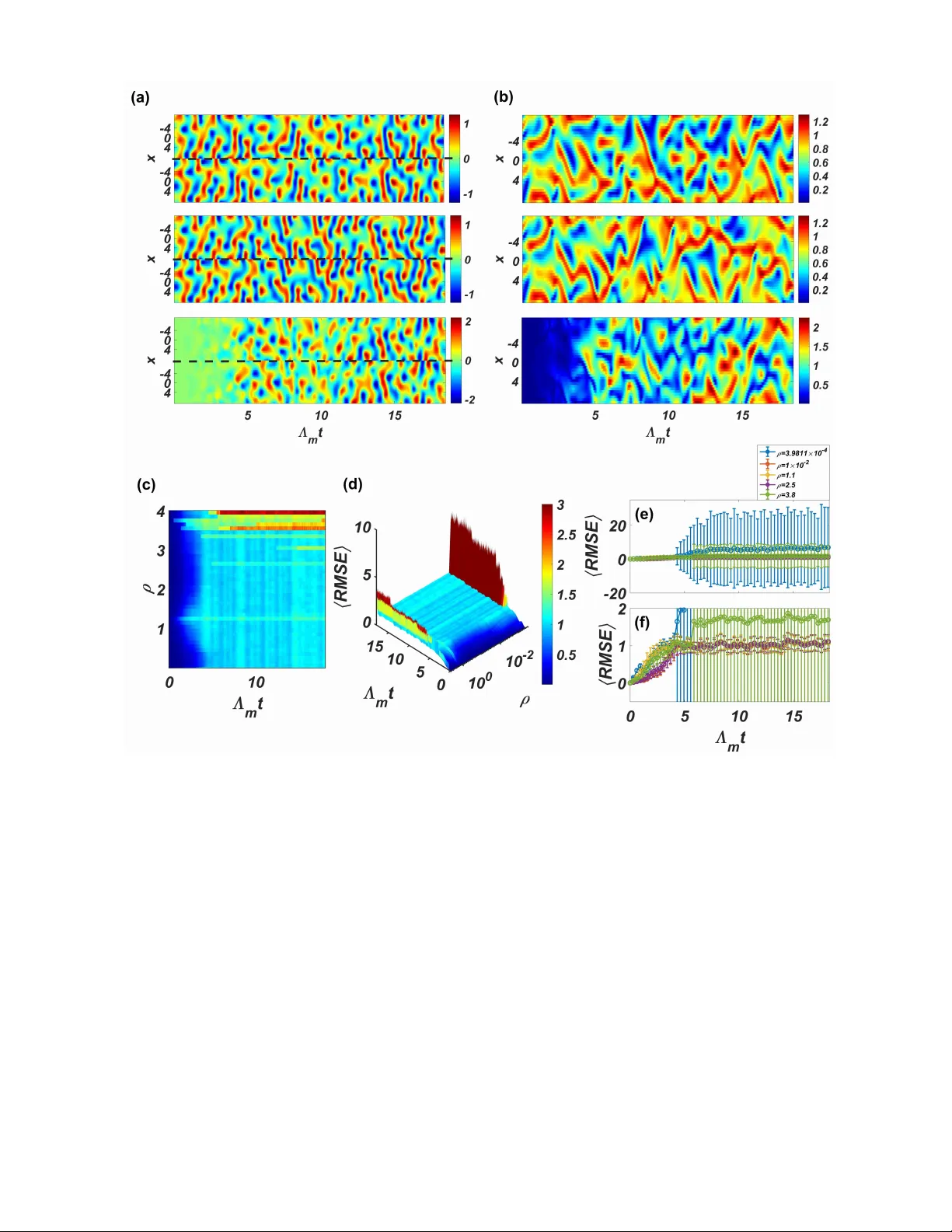
Loading high-quality paper...
Comments & Academic Discussion
Loading comments...
Leave a Comment