An Interactive Control Approach to 3D Shape Reconstruction

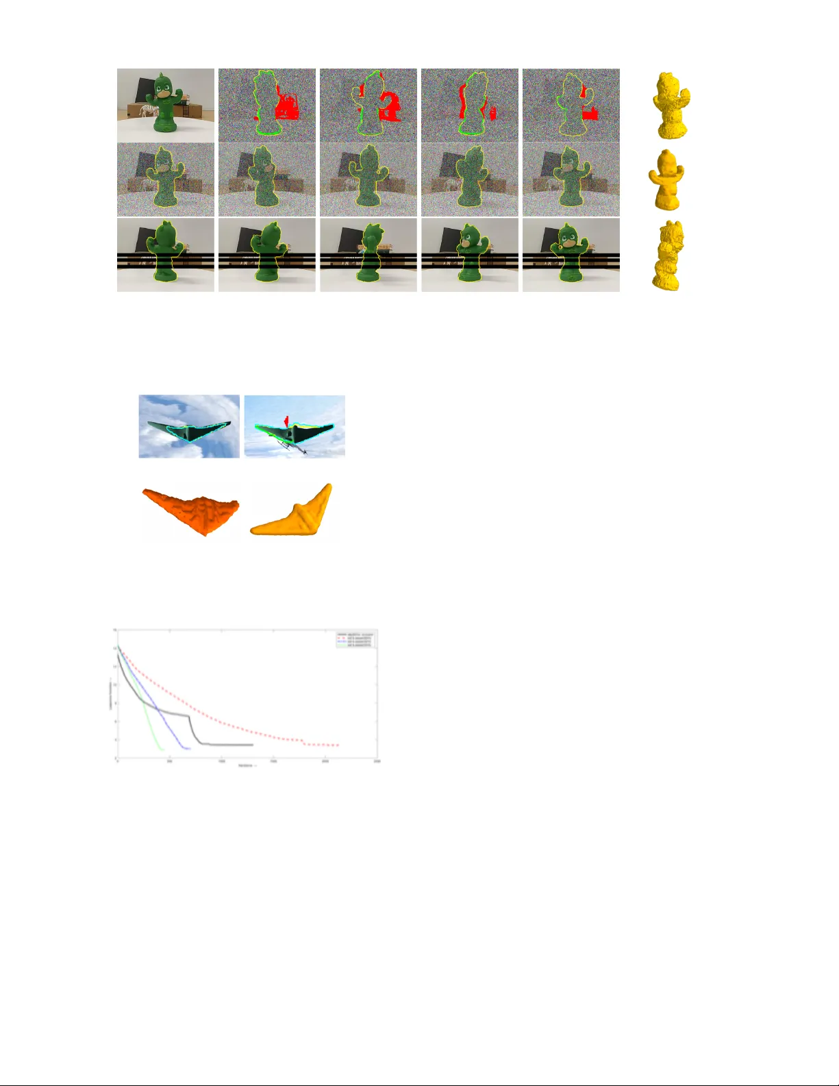
Interactiv e Contr ol A ppr oach to 3D Shape Reconstruction Bipul Islam, Ji Liu, Anthony Y ezzi, Romeil Sandhu Abstract — The ability to accurately reconstruct the 3D facets of a scene is one of the key problems in robotic vision. Howev er , even with r ecent advances with machine lear ning, there is no high-fidelity universal 3D reconstruction method for this optimization problem as schemes often cater to specific image modalities and are often biased by scene abnormalities. Simply put, there always remains an “information” gap due to the dynamic nature of real-world scenarios. T o this end, we demonstrate a feedback control framework which in v okes operator inputs (also prone to errors) in order to augment exist- ing reconstruction schemes. For proof-of-concept, we choose a classical region-based stereoscopic reconstruction approach and show how an ill-posed model can be augmented with operator input to be much more rob ust to scene artifacts. W e pr ovide necessary conditions for stability via L yapunov analysis and perhaps more importantly , we show that the stability depends on a notion of absolute cur vature. Mathematically , this aligns with previous work that has shown Ricci curvatur e as proxy for functional rob ustness of dynamical networked systems. W e conclude with results that show how our method can improve standalone reconstruction schemes. I . I N T RO D U C T I O N Sensing the spatial particulars and inferring information about a real-world scene from images is a classical problem in robotic vision with a multitude of uses ranging from motion planning, situational awareness, to medical imaging [1], [2], [3]. This said, reconstruction of a complex 3D scene from 2D images is a dif ficult task due to the amount of uncertainties that must be accounted for in real-world scenarios. Although much progress ha ve been made ov er the last few decades, reconstruction methodologies often fail as a result of imaging artifacts including, b ut not limited to, noise, occlusions, clutter , and non-uniform illumination. In short, no univ ersal algorithm exists which can work seamlessly across all image modalities [4]. T o combat such risk complexities, there is a need for domain e xperts or an operator who is able to provide an estimate of the ideal result and subsequently able to verify the quality of reconstruction. Here, we aim to “inject” 2D operator inputs in-loop to dri ve a (multi-agent) 3D surface deformation while ensuring the resulting system is stable in the sense of L yapuno v [5]. While this work builds off of our previous work in image segmentation [4] and reconstruction [1], there lies a few tacit yet important discerning cav eats. Firstly , we show that 2D operator inputs of a gi ven set of images can be aptly “mapped” to 3D world and such inputs, are stable. Mathematically , this not B. Islam and R. Sandhu are with the Department of Computer Science & Biomedical Informatics and J. Liu is with the Department of Electrical and Computer Engineering, Stony Brook University , Stony Brook, NY 11794. A. Y ezzi is with the Department of Electrical and Computer Engineering, Georgia T ech, Atlanta GA, 30309. R. Sandhu is also with the Departments of Applied Mathematics & Statistics, Stony Brook Uni versity , Ston y Brook, NY 11794. E-mail: bipul.islam@stonybrook.edu Fig. 1: Schematic outline of interacti ve feedback control stereoscopic reconstruction framework. a trivial issue as an y input on a 2D background should also be corroborated by a 3D action on infinitely large (“blue sky”) background (e.g., specifying the 3D action location based on 2D background input is ill-posed). From a stability perspectiv e, such singular 2D actions affect not only a 3D surface deformation, b ut indirectly affect other 2D passiv e sensors via 3D-to-2D projections during the reconstruction process. Secondly , the control laws are de veloped in-part based on a notion of absolute principle curvature which is a main underlying theme of this work (e.g., confluence of geometry & control). Thirdly , curvature can be shown to relate to a notion of “trust” in the sense of how quickly our reconciled solution con ver ges from both the operator and autonomous perspectiv e. This will be stylized in detail in future work, but is presented here to place this work and contributions in context. W e no w briefly revisit a fe w techniques as it pertains to this work. A. Brief 3D Reconstruction Literatur e Revie w Most modern scene reconstruction methods use the pop- ular deep (reinforcement) learning variants and are often characterized by the requirement of massiv e training samples [6], [7]. Some examples of such systems are ScanNet [6] that uses over 2.5 million scenes to train a system that can understand indoor scenes to [7] where authors furnish a synthetic dataset in order to develop an understanding of surface normal prediction, semantic segmentation, and object boundary detection. Generally , such schemes are highly dependent on the training quality . T o combat this, [8] explores the use of supervision as an alternativ e for expensi ve 3D annotation from which perspectiv e projection and back propagation are employed. On the other hand, such methods use local correspondence matching and hence, are fallible to dra wbacks resulting from scene abnormalities (e.g., noise, non-uniform illumination [9]). In regards to robotic vision, such correspondence-based solutions generally in volv e the well-known concept of SLAM (Simultaneous Localization and Mapping) [10], [11], [12]. This said, SLAM-based methods traditionally suffer from the requirement of high computational power for sensing a sizable area and process the resulting data to perform both mapping and localization. Also, there is a tacit requirement that input scene images should ha ve overlap from image-to-image. T o this end, SFM (Structure From Motion) based methods provide a relaxed version of this problem [13], [14] (i.e., Google uses this approach in their popular street-view application on Google maps [15]). More recently , [16] explores a recurrent neural network (3D-R2N2) by employing shape priors in which one learns 2D to 3D mapping from images of objects to their underlying 3D shapes from large collections of synthetic data. In particular , the authors hav e been seemingly able to show their method outperforming SLAM or SFM (albiet with learnt knowledge) when there is lack of te xture or baseline. Nev ertheless, this paper does not argue the rigors of the underlying reconstruction method itself and our par- ticular focus on our previous work [1] is in-part due a correspondence-free method, independence to local (image- gradient) structure, and dependence on geometric techniques connected to image segmentation [17], [21], [22]. Undoubt- edly , each approach whether it be SLAM-based, deep (re- inforcement) learning variants, and/or geometric methods work optimally with respect to the prospective operating en vironment (e.g., space, low-po wer requirements compared ground-based robotic vision). At the same time, any such reconstruction are not infallible to errors that arise in real- world dynamic scenes from a human-perception standpoint. This said, human-perception is also fallible and an y operator input based on a visual estimate is prone to errors. Philo- sophically , we make the argument that terms such as over - fitting and uncertainty are in part, percei ved by an expert who generally acts as a passive entity in such methods. Thus, the problem we seek to resolve is to not only rectify the expected and ideal reconstruction in real-time [23], but provide the necessary feedback control characterization when inv oking operator input [24]. The remainder of the paper is org anized as follows: In the next, we introduce stereoscopic reconstruction via classic image segmentation. Then Section III provides a control framew ork along with the necessary conditions for stability . Section IV presents experimental results. From this, we conclude with future work in Section V . I I . F RO M S E G M E N TA T I O N T O 3 D R E C O N S T RU C T I O N This section presents a general introduction to geometric stereoscopic segmentation. A. Geometric 2D Image Segmentation Let us be gin with the classic binary problem of segmenting an image I : Ω 7→ R n into a foreground and background described by functionals r o : ζ , Ω 7→ R and r b : ζ , Ω 7→ R which measure the similarity of of the image pixels with a statistical model over the regions R and R c , respectively . Here, ζ corresponds to the photometric v ariable of interest. Then, one can define a partitioning problem where the op- timal partition between foreground/background is described by a partial dif ferential equation [22], [26]; i.e., E = Z R r o ( I ( x ) , C ) + Z R c r b ( I ( x ) , C ) d Ω (1) ∂ E ∂ C = β ~ N where β : R 2 7→ R can be considered “forces” along the curve (partition boundary) that describe the direction of the corresponding ev olution in the normal ~ N direction. While a complete revie w of such methodology is beyond the scope of this note, we do refer the reader to several seminal references [17], [21]. For the case image segmentation, it suf fices to understand that the partitioning curve C “lives” in the 2D image domain. B. Stereoscopic 3D Reconstruction Now , if we consider the problem of 3D reconstruction from 2D images, one can redefine the functional in equation (1) as follows: E = N ∑ i = 0 Z R i r o ( I i ( ˆ x i ) , π − 1 i ( ˆ x i ) , ˆ c i ) + Z R c i r b ( I i ( ˆ x i ) , Θ i ( ˆ x i ) , ˆ c i ) d Ω i (2) where the difference is the functional now depends on N image observations I i and where a particular 2D image silhouette curve ˆ c i is derived from a single 3D occluding curve C (with a slight abuse of notion) on a given smooth surface S in R 3 with a corresponding 3D background B treated as infinitely large sphere with angular coordinates Θ = ( γ , υ ) . That is, ˆ c i = π i ( C ) where π i : R 3 7→ Ω i is the realization of the i -th pin-hole camera (sensor) that projects the 3D world onto the 2D domain. Similarly , the background can be related in a one-to-one manner with the image coordinates ˆ x i of each observation through the mapping Θ i (“blue sk y” assumption). T o be more precise, x = ( x , y , z ) is surface coordinates of S in R 3 and further note that x i = ( x i , y i , z i ) denote the same points expressed in i -th calibrated camera coordinates relati ve to the i -th image. Moreov er , ˆ x i = ( ˆ x i , ˆ y i ) = ( x i / z i , y i / z i ) is the aforementioned perspectiv e projection due to the i -th pin-hole camera π i . In turn, r o and r b redefined to be radiance functions. That is, the foreground object of interest supports a radiance function of r o : S → R with the usual area element d A . Similarly , the background supports a different radiance function r b : B → R . As such, for a giv en 3D surface, it is possible to partition each image domain Ω i of I i into a foreground object region R i = π i ( S ) ⊆ Ω i and the corresponding background region R c i . Note, the operator π i is not one-to-one and, hence non- in vertible. Ho we ver , we can define a back projection operator π − 1 i using the back tracing of rays from image to the surface, i.e, we hav e π − 1 i : R i → S which is a pseudo one-to-one operation. Fig. 2: V isualization of Normal, Principle, and Gaussian Curvature. (A) Gi ven Point P and Normal N , define a per- pendicular plane intersection at point P . The curve that plane intersects on the manifold is known as the normal curvature κ X in the direction X . (B) W e can define other normal curvatures through a rotation of the plane by θ . (C) The max and min normal curvature are what is known as principle curvatures. The product of these principle curv atures yields Gaussian curvature. Putting this together, assuming the calibrated cameras, the deformation of the surface towards a reconstructed shape based on a set of N image observ ations can be shown to be of the follo wing form: ∂ S ∂ t = N ∑ i = 0 β i ·  ∇ x i χ i · x i z 3 i  ~ N where we define a visibility characteristic function χ i from a giv en location x i on a surface S as: χ i ( x x x ) = ( 1 , if x i ∈ π − 1 i ( R i ) 0 , if x i / ∈ π − 1 i ( R i ) . This can be re-written in terms of the smooth regularized- Heaviside function H along with (outward) surface normals ~ N at each point x i of the surface S : χ i = 1 − H ( x i · ~ N ) Giv en the abov e, we are now able to formulate a control- based reconstruction scheme from which a giv en physical 2D action, based on visual perception (information), can be used to interactiv ely “sculpt” a 3D shape in collaboration with the above autonomous 3D reconstruction algorithm. I I I . C O N T RO L - B A S E D R E C O N S T R U C T I O N Let us begin by redefining the general form of a surface reconstruction e volution abov e in level-set notation as fol- lows: d φ d t = N ∑ i = 0 ψ i ( ˆ x i , x i , t ) δ ( φ ( x )) (3) where ψ i : R 3 → R is the surface gradient information computed from the photometric image data, φ : R 3 → R is a lev el-set function, and δ ( . ) is the classical Kronecker delta function. Hence, to “close the loop” that incorporates a physical 3D operator performing 2D inputs in order to control the 3D ev olution dynamics of the e volving surface, one has d φ d t = N ∑ i = 0 [ ψ i + F i ( φ , φ ∗ )] δ ( φ ) (4) where F i is the to be defined control law that dri ves φ tow ards the ideal (perfect) surface φ ∗ as t → ∞ . The definition of an ideal surface is this note is a result with no errors. For this work, we use the mean-separable segmentation energy [21] as our reconstruction model. From this, ∇ x i χ i · x i can be expressed in terms of curvature for points on the surface which leads us to the follo wing Lemma. Lemma III.1 F or a given characteristic function χ i and a point x i ∈ S that lies on the corr esponding surface “imag ed” fr om a given camera π i , we have that ∇ x i χ i · x i = − κ u k x i k 2 δ ( x i · ~ N ) . (5) Pr oof: Following the nomenclature defined abo ve and noting II ( x x x , x x x ) is the second fundamental form [14], [27], we hav e ∇ x i χ i · x i = h ∇ x i ( 1 − H ( x i · ~ N )) , x i i = −h δ ( x i · ~ N ) ∇ x i ( x i · ~ N ) , x i i = − δ ( x i · ~ N ) h ∇ x i ( x i · ~ N ) , x i i = − δ ( x i · ~ N )( ∇ x i ~ N T x i ) T x i = − δ ( x i · ~ N )[ x i T ∇ x ~ N x i ] = − δ ( x i · ~ N )  u v   l m m n   u v  = − δ ( x i · ~ N ) II ( x i , x i ) = − δ ( x i · ~ N ) II ( x i , x i ) x i T x i k x i k 2 = − δ ( x i · ~ N ) κ u k x i k 2 (6) where k u is the normal curv ature in a particular viewing dir ection x i on the corresponding surface S . W e refer to Figure 2 for a visualization of this type of curvature on a given manifold. From this, we can rewrite ψ i as the following: ψ i = − β i δ ( x i · ~ N ) κ u k x i k 2 z 3 i . (7) Furthermore, as we aim to define a control law F i such that lim t → ∞ φ ( x x x ) → φ ∗ ( x x x ) , we define the error between our current estimate and ideal shape (no errors) as E e ( x , t ) : = H ( φ ( x , t )) − H ( φ ∗ ( x )) . (8) In doing so, we are no w able to define the existence of the control law F i via L yapuno v method of stabilization. Theorem III.1: Let us assume z i ≥ 1 and || x i || 2 ≤ z 3 i as well as let κ max and κ min be the the principle maximum curvature and principle minimum curvature at a given point x i with r espect to an imaging r efer ential camera π i , r espectively . Then the control law F i = − | β i | κ abs E e (9) wher e κ abs = | κ min | + | κ max | , asymptotically stabilizes the system given in equation (4) fr om the curr ent evolving surface φ ( x x x , t ) to the ideal surface, φ ∗ ( x x x ) as t → ∞ . Pr oof: W e choose the L yapuno v function V ( E e , t ) ∈ C 1 defined in terms of E e ( x , t ) as V = 1 2 Z S ∪ S ∗ k E e ( x , t ) k 2 d x . (10) Differentiating V with respect to time t we get: ∂ V ∂ t = Z S ∪ S ∗ E e ∂ E e ∂ t d x = Z S E e [ δ ( φ ) ∂ φ ∂ t ] d x = Z S E e δ ( φ )[ N ∑ i = 0 [ ψ i + F i ] δ ( φ )] d x (11) The simplification over the union S ∪ S ∗ results from the application of the Kronecker delta function. Moreov er , one can sho w that resulting system is stable (i.e., V has a ne gati ve semidefinite deriv ati ve): ∂ V ∂ t = N ∑ i = 0 Z S E e δ ( φ ) 2 [ ψ i + F i ] d A = N ∑ i = 0 Z S E e δ ( φ ) 2  β i · ∇ x i χ i · x i z 3 i + F i  d A = N ∑ i = 0 Z S E e δ ( φ ) 2  β i · ∇ x i χ i · x i z 3 i − | β i | κ abs E e  d A = N ∑ i = 0 Z S δ ( φ ) 2  E e · β i · ∇ x i χ i · x i z 3 i − | β i | κ abs E 2 e  d A ≤ N ∑ i = 0 Z S δ ( φ ) 2  E 2 e · | β i |     ∇ x i χ i · x i z 3 i     − | β i | κ abs E 2 e  d A = N ∑ i = 0 Z S δ ( φ ) 2 E 2 e | β i |      ∇ x i χ i · x i z 3 i     − κ abs  d A = N ∑ i = 0 Z S δ ( φ ) 2 E 2 e | β i |  | κ u k x i k 2 z 3 | − κ abs  d A < N ∑ i = 0 Z S δ ( φ ) 2 E 2 e | β i |  | κ u | − κ abs  d A ≤ 0 In particular, the above control law will be dependent on curvature. While be yond the scope of this note, one can show exponential conv ergence whereby higher curvature coincides with faster con ver gence rates. While we have not included this deri vation in the present work due to scope and for sake of clarity , we will expound upon this in future work. This said, we present such comments to better highlight important cav eats in terms of geometry and control as well as how one can start to define notions of “trust” (from a reconciliation of an operator augmentation) to that of a geometric (curv ature) quantity . W e would like to highlight there exists analogous behavior in networked dynamical systems in which one is able to use discrete Ricci curv ature as a measure for network robustness [28]. In such work, one can leverage the concept of k-conv exity similarly to above to define positiv e correlation between Boltzmann entropy , curvature, and rate functions from thermodynamics. Ultimately , this (a) Incision (b) Repair (c) Consolidate (d) Final Fig. 3: A summary of operators actions to maneuver out of the local minima in a complex occluded scene. The images (A), (B), and (C) are views of the model after each of interaction milestones. Sub-figure (C) shows the final reconstruction. work will seek to build upon this area and in particular , explore notions of “trust” in the sense of geometric quantities such as curvature. Nev ertheless, in designing operator guided inputs, we note perfect knowledge of ideal surface is not readily av ailable (ev en from a human visualization perspective) due a myriad of reasons including, but not limited to, occlusions, clutter, and/or inability to define a well-posed model across image modalities. As such, we allow an operator (whom is also prone to errors) to make interactions with the system in order to reconcile one’ s belief with b uilt autonomy tow ards an estimate of the ideal surface. W e stress the fact that the input from a human is fallible and such input indirectly affects our control law through the adjudication of an “ideal” estimate. This estimate herein is denoted as ˆ φ ∗ ( x , t ) . Moreov er , we define ε k i ( ˆ x i , t ) as the k -th input on a giv en image i and the accumulated input U i : R 2 → R as ε k i ( ˆ x i , t ) : = ± p (constant) U i ( ˆ x i , t ) : = k ∑ l = 0 ε k t ( ˆ x i ) . That is, we seek to allow for the physical operator to make 2D actions such that it will deform a 3D surface . In other words, we are able to define a 3D control law based on 2D inputs which is particularly helpful as the operator is generally ill-equipped to alter the 3D shape itself (i.e., we assume the operator not to be an artist). T o deriv e the coupled system that fuses 2D operator input to control the 3D surface deformation, we must also define the errors for both the operator and autonomous model: E A = H ( φ ( x ) , t )) − H ( ˆ φ ∗ ( x ) , t )) E u i = H ( ˆ φ ∗ ( x x x ) , t )) − H ( U i ( π i ( x x x ) , t )) . (12) Giv en this, we can no w define a coupled PDE system that unifies both the operator based inputs along with that of the autonomous counterpart which is representativ e of an estimator-observ er behavior as follows: ∂ φ ∂ t = N ∑ i = 1 [ ψ i + F i ] δ ( φ ) (13a) φ ( x , 0 ) = φ 0 ( x ) ∂ ˆ φ ∗ ∂ t = N ∑ i = 1 [ E A + f i ( U i , E u i )] (13b) ˆ φ ∗ ( x , 0 ) = φ 0 ( x ) where the tuning function f i ( U i , E u i ) that is dependent on operator input from an image observ ation can be defined as f i ( U i , E u i ) = − | U i | E u i . (14) This said, the above system then needs to be sho wn that it is is still stable e v en from imperfect operator actions. T o do so, we define the accumulated total errors for both the operator and autonomous model as E ( t ) : = 1 2 N ∑ i = 1 Z S ∪ B | U i | E 2 u i d x (15) Γ ( t ) : = 1 2 N ∑ i = 1 Z S ∪ S ∗ E 2 A . (16) From this, we no w arriv e at the follo wing result. Theorem III.2: Let us assume pr evious notation and r esults in Theor em III.1 and further assume that operator input has stopped (i.e., U i is constant in all viewing directions), then the estimator ∂ ˆ φ ∗ ∂ t = N ∑ i = 1 [ E A + f i ( U i , E u i )] wher e f i ( U i , E u i ) = − | U i | E u i will stabilize the r esulting cou- pled system in equation (13a) and equation (13b). Namely , the total err or Φ ( t ) : = E ( t ) + Γ ( t ) has a ne gative semidefinite derivative. Pr oof. Let us begin by differentiating E ( t ) with respect to t : ∂ E ∂ t = N ∑ i = 1 Z S ∪ ˆ S ∗ | U i | E u i ∂ E u i ∂ t = N ∑ i = 1 Z S ∪ ˆ S ∗ | U i | E u i δ ( ˆ φ ∗ ) ∂ ˆ φ ∗ ∂ t d x = N ∑ i = 1 Z S ∪ ˆ S ∗ | U i | E u i δ ( ˆ φ ∗ )[ E A − | U i | E u i ] d x . (17) Similarly , dif ferentiating Γ ( t ) with respect to t : ∂ Γ ∂ t = N ∑ i = 1 Z S ∪ ˆ S ∗ E A  δ ( φ ) ∂ φ ∂ t − δ ( ˆ φ ∗ ) ∂ ˆ φ ∗ ∂ t  d x = N ∑ i = 1 Z S ∪ ˆ S ∗ δ ( φ ) 2 E A [ ψ i + F i ] d x − N ∑ i = 1 Z S ∪ ˆ S ∗ δ ( ˆ φ ∗ ) 2 E A [ E A − | U i | E u i ] d x . (18) Fig. 4: The overall sequence w .r .t. to energy minimization of operator action corresponding to Figure 3b. (A ) Incision, (B) Repair , (C) Consolidate. From this, we are now able to combine terms for the total labeling error Φ ( t ) = E ( t ) + Γ ( t ) . That is, summing equation (17) and equation (18) and simplifying: ∂ Φ ∂ t = N ∑ i = 1 Z S ∪ ˆ S ∗ | U i | E u i δ ( ˆ φ ∗ )[ E A − | U i | E u i ] d x + N ∑ i = 1 Z S ∪ ˆ S ∗ δ ( φ ) 2 E A [ ψ i + F i ] d x − N ∑ i = 1 Z S ∪ ˆ S ∗ δ ( ˆ φ ∗ ) 2 E A [ E A − | U i | E u i ] d x ≤ − N ∑ i = 1 Z S ∪ ˆ S ∗ δ ( ˆ φ ∗ ) 2 [ E A − | U i | E u i ] 2 d x ≤ 0 (19) As the deriv ati ve is ne gativ e semidefinite, the coupled system defined above is stable. I V . E X P E R I M E N TA L R E S U LT S A N D D I S C U S S I O N In this section, we demonstrate the proposed algorithm on a variety of scenarios. In all demonstrated results, green patches, or marks, are made by the user to denote re gions in the foreground. Similarly , red denotes regions on images that are to be considered a part of the background. In images where silhouettes are displayed, the yello w silhouette denotes the autonomous surf ace while the estimate of ideal surface is always presented in cyan. Each reconstruction utilizes N = 36 images with the resulting MA TLAB code run on an iMac 4.2 Ghz Core i7 with 32GB memory . W e begin with an e xample that highlights the method in face of occlusions by objects obfuscating sev eral different imaging views. This can be seen Figure 3 along with how such inputs affect the energy minimization landscape in Figure 4. Here, naiv e reconstruction fails due to ambient occlusion whose intensity is similar to the background. While there exists varying approaches and shape prior models to overcome such a problem, defining such models for particular scenarios becomes quite cumbersome and yet, may not yield stable results. W e are able to properly reconstruct the shape through operator input with a simplified model as defined in [21]. For this experiment, the user made 12 Fig. 5: 3D reconstruction of a cup in clutter and camera miscalibration. T op ro w: Sequence of user initiated operations to reorient the flow at multiple time instances. Bottom row: Final silhouette curves and reconstruction. Note: Y ello w Curve is Autonomous Surface, Blue Curve is Ideal Estimate, Green is F oreground Interaction, Red is Background Interaction. interactions for the foreground and 47 interactions for the background. In particular , in regards to the operator input and its impact on the energy landscape, the user actions can be partitioned into 3 milestones: initial incision (Figure: 3a), followed by a repair of the surface (Figure: 3b), and then, consolidating the surface by helping it “free” itself from scene anomalies (Figure: 3c). More importantly , irrespectiv e of the underlying model chosen for reconstruction, there will exist assumptions that are violated possibly due v ariety of image artifacts such as noise, clutter , and/or model assumptions itself . That is, for the chosen reconstruction autonomous model, we make the classic assumption that the scene is “mean-separable” and piecewise constant. Of course, while there exists other more advances models, such a model helps illustrate where opera- tor feedback may ov erride basic fallible assumptions. Figure 8 presents a scene in which such piecewise assumption is violated along minor camera miscalibrations. Additional scenes for which such assumption is violated can be seen in Figure 7 which aims to reconstructs a predator drone in a seemingly distinguishable background of clouds yet fails without operator input. In the context of stereoscopic reconstruction, overcoming non-uniform illumination is yet another tacit challenge. Figure 9 presents a scene where reconstruction of a sentinel drone fails due to tacit illu- mination on the ailerons that varies over the dataset. This is in part, due to illumination on the left wing which is consequently lo wer than the right wing. Utilizing operator input, the reconstruction results are demonstrated. T o further the idea in a quantitive non-subjective man- ner , we conduct numerical noise e xperiments on reconstruc- tion of a synthetic scene of a sentinel drone which can be seen in Figure 6 and T able I. Ultimately , if the operator requires intensi ve work to assist the autonomous counterpart in such situations, then manual operator would suffice (or desire for improved built autonomy). This said, T able I presents efficiency results as the amount of user input is needed (in terms of % “actions” per view , % relabeling of pixels) compared to increased output (in terms of true and false positiv e rate pixel labels). For example, the second row can be stated that under 30% noise with only one action (user-input) on 95% of the views which amounts to only 2.7% pixel relabeling per image view , the true positive rate increases from 78.4% to 99.2%. This is repeated on sev eral versions of noise and occlusion, two of which are seen from different vie ws in Figure 6. Nevertheless, the ke y application point of view her e is that such failures of such r econstruction methods due to imaging artifacts such as noise can be naturally r ecover with minimal effort with human in-loop collaboration. In addition to such results, we provide corresponding L yapunov decay rates to such scenes in Figure 10. Lastly , we note significant work on methods that use “feature”-based methods that rely on correspondences com- bined with machine learning to perform reconstruction tasks [6], [9], [8], [12]. While the thematic aspect of this paper is not discuss the rigors of such methods compared to the proposed underlying autonomous method, it is worthwhile to note that under such noisy situations, such correspondence methods (dependent on structural image information) began to suffer . Here, the geometric method proposed can be considered a “coarse” approach to tackle such “featureless” en vironments. This said, future work will focus on fusing such correspondence-based and learning approaches in hopes to define a notion of image integrity and le verage recent learning success on data that is indeed well-structured. V . C O N C L U S I O N S A N D F U T U R E W O R K S In this paper , we hav e proposed a feedback control framew ork to guide the dynamics of an e volving surface in the context of multi-view stereoscopic reconstruction. This is done to ensure robustness in presence of lo w-fidelity datasets. From an optimization standpoint, the reconstruction Fig. 6: V isual Synthetic Sentinel Drone Reconstruction Under Noise Conditions Corresponding to T able I. T op Row: Several V iews Showing 90% Noise. Bottom Ro w: Se veral V iews Showing 50% Noise with 37% Occlusion Ov er Image Domain. Fig. 7: Example where interactions are added to the wing- tips which are darker than ambient clutter of clouds and additional shape complication due drone thinness in wings. minima which we often seek (due to modeling imperfections) may not coincide with user expectations. As opposed to defining complex models for which overfitting may arise, we incorporate a user-defined input in-loop and “on-the-fly” from a feedback control perspecti v e. W e sho w the resulting framew ork is stable via L yapunov analysis and from a practical standpoint, there is an increase in efficiency through a human-autonomous collaboration in shape reconstruction. Mathematically , the thematic interest is the interplay of geometry and control, namely how notions of curv ature from geometry infer con ver gence and for this note, a notion of autonomous trust to user-input. This said, future work will entail a much closer analysis in regards to how Gaussian curvature infers con v er gence as well as the study of a problem in a distributed optimization sense, non-constant and time-delayed inputs as well as the inclusion of stochastic optimal control to further characterize operator uncertainty . R E F E R E N C E S [1] A. Y ezzi and S. Soatto. “Stereoscopic Segmentation. ” International Journal of Computer V ision . 2003 [2] O. Faugeras and R. Keriv en. V ariational Principles, Surface evolu- tion, PDE’s, Le vel Set Methods and the Stereo pr oblem , INRIA . 1996. Noise Interactions % Pixels T rue False % V iew Pos. Rate Pos. Rate 30% (0, 0) 0% 78.4% 0.96% 30% (1, 95%) 2.7% 99.2% 3.09% 50% (0, 0) 0% 47.6% 0.2% 50% (1, 95%) 2.7% 99.8% 4.8% 90% (0, 0) 0% 21.8% 1% 90% (1, 95%) 2.7% 99.9% 14.3% 90% (1, 36%) (2, 60%) 6.3% (2.7+3.6) 99.9% 4.92% noise: 50%+ occlusion: 37% (1, 36%) (2, 60%) 6.7% (2.7+4) 99.6% 4.3% T ABLE I: Comparativ e analysis with noise and occlusion for the synthetic example of the Sentinel drone. [3] F . Zhao and X. Xie. “ An Overvie w of Interacti ve Medical Image Segmentation”, Annals of the BMV A . 2013 [4] L. Zhu, P . Karasev , I. Kolesov , I, R. Sandhu, and A. T annenbaum. “Guiding Image Segmentation On The Fly: Interactive Segmenta- tion From A Feedback Control Perspective”, IEEE T ransactions on Automatic Contr ol . 2018. [5] K. Khalil. “Nonlinear systems”, Pr entice-Hall, New J erse y . 1996. [6] A. Dai, A. Chang, M. Savv a, M. Halber , T . Funkhouser, and M. Nießner . “ScanNet: Richly-Annotated 3D Reconstructions of Indoor Scenes”, CVPR . 2017. [7] Y . Zhang, S. Song, E. Y umer , M. Savva, J. Lee, H. Jin, and T . Funkhouser . “Physically-Based Rendering for Indoor Scene Under- standing Using Con v olutional Neural Networks”, CVPR . 2017. [8] J. Gwak. C. B. Choy , M. Chandraker, A. Garg, and S. Sav arese. “W eakly Supervised 3D Reconstruction with Adv ersarial Constraint”, 2017 International Confer ence on 3D V ision . 2017. [9] Z. Chen, X. Sun, L. W ang, Y . Y u and C. Huang. “ A Deep V isual Correspondence Embedding Model for Stereo Matching Costs”, CVPR . 2015. [10] J. Aulinas, Y . Petillot, J. Salvi, X. Llad ´ o. “The SLAM Problem: A Survey”, CCIA . 2008. [11] G. Zhang, and P . V ela. “Optimally Observable and Minimal Cardi- nality Monocular SLAM”, ICRA . 2015. [12] Y . Zhao and P . V ela. “Good Line Cutting: T owards Accurate Pose T racking of Line-assisted VO/VSLAM”, ECCV . 2018. [13] A. Y ezzi and S. Soatto. “Structure from Motion for Scenes without Features”, CVPR . 2003. [14] O. Faugeras. “Three-Dimensional Computer vision: a Geometric V ie wpoint”, MIT Pr ess . 1993. [15] B. Klingner, D. Martin, and J. Roseborough. “Street V iew Motion from Structure From Motion”, CVPR . 2013. Fig. 8: 3D Reconstruction of a T oy Figurine. T op Ro w , First Image: Original Image of One V ie w . T op Ro w: Significant Noise Applied to All V ie ws with 3D Reconstruction. Middle Row: Moderate Noise Applied to All V ie w with 3D Reconstruction. Bottom Ro w: Induced Camera Artifacts with 3D Reconstruction. Note: The underlying algorithm assumes object and background are “mean-separable” (e.g., such scenes are dif ficult corresponding to underlying autonomous model). (a) (b) (c) (d) Fig. 9: Complications due to v aried illumination conditions where interactions are added to the left wing-tip. Fig. 10: L yapunov function decay plots of noise scenes. Black: 50% Noise with Occlusion. Red: Noise at 90%. Blue: Noise at 50%. Green: Noise at 30%. The “knee-like” decrease in error in black/red signals are due to user-input. [16] C. Choy , and D. Xu, J. Gwak, K. Chen, and S. Sav arese. “3d- r2n2: A Unified Approach for Single and Multi-Vie w 3D Object Reconstruction”, ECCV . 2016 [17] D. Mumford and J. Shah. “Optimal Approximations by Piecewise Smooth Functions and Associated V ariational Problems”, Communi- cations on Pur e and Applied Mathematics .1989. [18] K. Kutulakos, N. Kiriakos, and S. Seitz. “ A Theory of Shape by Space Carving”, International Journal of Computer V ision . 2000. [19] A. Mulayim, U. Y ilmaz, and V . Atalay . “Silhouette-Based 3D Model Reconstruction From Multiple Images”, IEEE T ransactions on Sys- tems, Man, and Cybernetics . 2003. [20] M. Jancosek and T . Pajdla. “Se gmentation Based Multi-V ie w Stereo. ” Computer V ision W inter W orskhop . 2009. [21] T . Chan and L. V ese. “ An Activ e Contour Model Without Edges”, In- ternational Conference on Scale-Space Theories in Computer V ision . 1999. [22] M. Bertalmıo, L. Cheng, S. Osher and G. Sapiro. “V ariational Problems and Partial Differential Equations on Implicit Surfaces”, Journal of Computational Physics . 2001 [23] T . Nguyen, J. Cai, J. Zhang, J. Zheng. “Robust Interacti ve Image Segmentation Using Con v ex Active Contours”, IEEE T r ansactions on Image Processing . 2012 [24] J. Doyle, B. Francis, and A. T annenbaum. “Feedback Control The- ory”, Courier Corporation . 2013. [25] R. Sandhu, S. Dambreville, A. Y ezzi, A. T annenbaum. “ A Nonrigid Kernel-Based Framework for 2D3D Pose Estimation and 2D image segmentation”, IEEE TP AMI . 2010. [26] S. Kichenassamy , A. Kumar , P . Olver , A.T annenbaum, A. Y ezzi. “Conformal Curvature Flows: From Phase Transitions to Activ e V ision”, Ar chive for Rational Mechanics and Analysis . 1996. [27] M. Do Carmo. “Differential Geometry of Curves and Surfaces: Revised and Updated Second Edition”, Courier Dover Publications . 2016. [28] R. Sandhu, T Georgiou, E Reznik, L. Zhu, I. K olesov , Y . Sen- babaoglu, and A. T annenbaum. “Graph Curvature for Differentiating Cancer Networks”, Scientific r eports . 2015. [29] B. Bamieh, F . Paganini, M Dahleh. “Distrib uted Control of Spatially In variant Systems” IEEE T A C . 2002.