Bio-inspired Learning of Sensorimotor Control for Locomotion

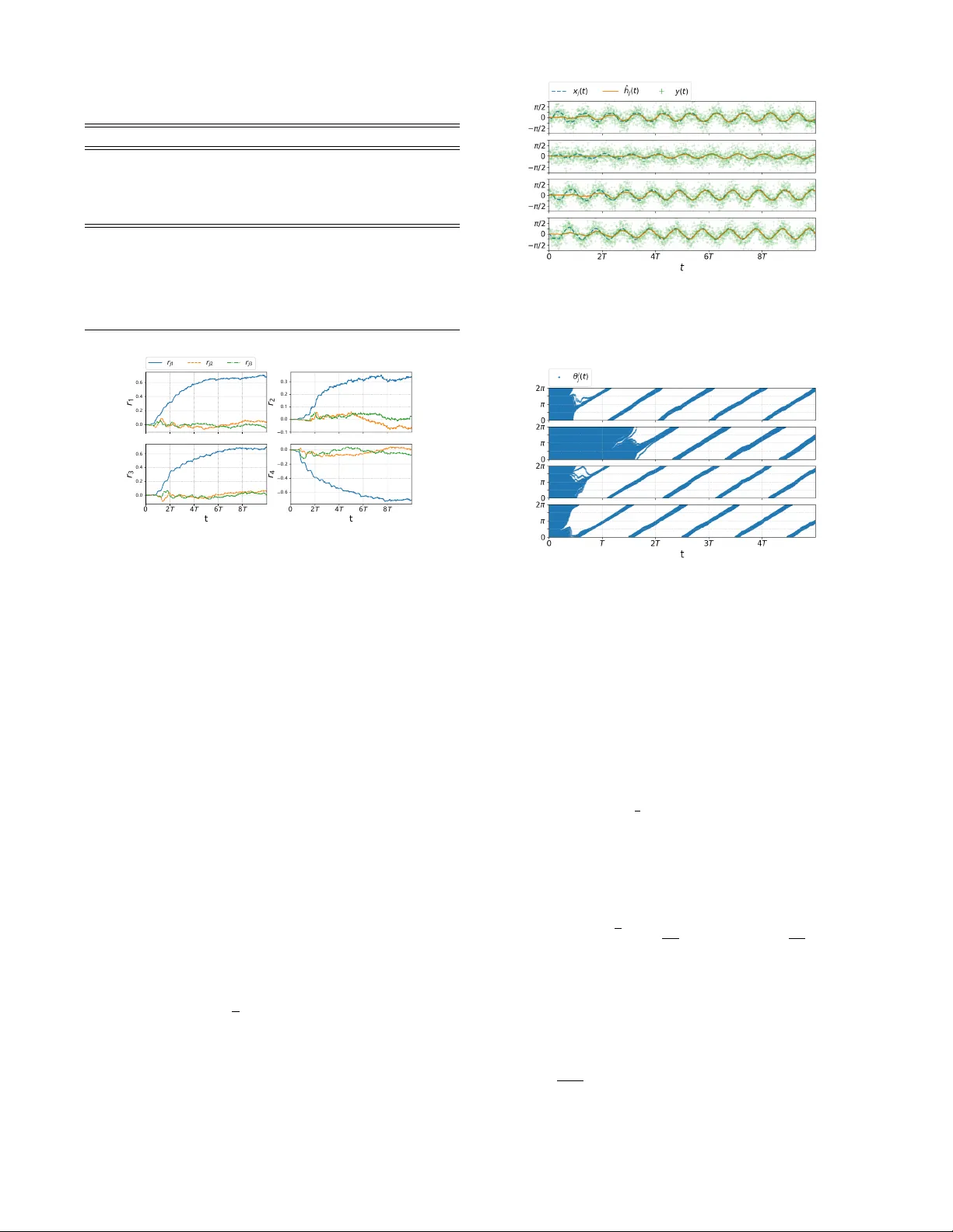
Bio-inspir ed Learning of Sensorimotor Contr ol f or Locomotion T ixian W ang, Amirhossein T aghv aei, and Prashant G. Mehta Abstract — This paper presents a bio-inspir ed central pattern generator (CPG)-type architecture for learning optimal maneu- vering control of periodic locomotory gaits. The architecture is presented here with the aid of a snake robot model problem in volving planar locomotion of coupled rigid body systems. The maneuver in volves clockwise or counterclockwise tur ning from a nominally straight path. The CPG circuit is realized as a coupled oscillator feedback particle filter . The collective dynamics of the filter are used to approximate a posterior distribution that is used to construct the optimal control input for maneuvering the robot. A Q-learning algorithm is applied to learn the approximate optimal control law . The issues surrounding the parametrization of the Q-function are discussed. The theoretical results are illustrated with numerics for a 5-link snake robot system. I . I N T RO D U C T I O N The objective of this paper is to present a bio-inspired central pattern generator (CPG)-type sensori-motor control architecture to learn optimal maneuv ers using only noisy sensor measurements and (online) rew ard. The dynamic and sensor models are assumed unknown. The architecture, depicted in Fig. 1, is presented here with the aid of a snake robot model problem inv olving planar locomotion of coupled rigid body systems. The snake robot is modeled as n coupled rigid bodies. The configuration space of the system is split into two sets of variables: (i) the shape variable which describes the internal shape of the system; (ii) and the gr oup v ariable which describes the global displacement and orientation of the system. The shape v ariables are actuated using motors at each joint to produce a nominal sinusoidal gait for the forward motion. The synthesis procedure for this gait is taken from [ 2 ], where it was shown to be optimal with respect to an energy cost function. The learning problem is for the robot to learn to maneuver about this nominal gait. The particular maneuver is to turn the robot either clockwise or counter-clockwise, e.g., to av oid an obstacle in the en vironment. W e assume noisy measurement of the shape v ariables and employ changes in friction coef ficients, with respect to the surface, as control inputs. The main comple xity reduction technique is to model the nominal periodic motion of the (local) shape variable at the j -th joint in terms of a single (hidden) phase variable θ j ( t ) for j = 1 , 2 , . . . , n − 1 . The inspiration comes from neuroscience Financial support from the ONR MURI grant N00014-19-1-2373 and the AR O grant W911NF1810334 is gratefully acknowledged. T . W ang, A. T aghvaei and P . G. Mehta are with the Coordinated Science Laboratory and the Department of Mechanical Science and Engineering at the Univ ersity of Illinois at Urbana-Champaign (UIUC). tixianw2@illinois.edu; taghvae2@illinois.edu; mehtapg@illinois.edu Fig. 1. The proposed architecture to learn a distributed feedback control law for turning the snake robot. where phase reduction is a popular technique to obtain reduced order model of neuronal dynamics [4]. A coupled oscillator feedback particle filter (FPF) is used to approximate the posterior distribution of θ j ( t ) giv en noisy measurements. The collecti ve dynamics of the ( n − 1 ) oscillator populations electrically encode the ev olution of the mechanical shape of the robot. The filter requires knowledge of the observation model which is also learned in an online fashion through the use of a linear parameterization. The filter outputs are aggregated into the second layer which seeks to learn the Q-function (or the Hamiltonian) based on an online access to the re ward. A cle ver linear parametrization is used to enforce a distributed architecture for the policy . The parameters are learned by using a gradient descent algorithm to reduce the Bellman error [12], [5]. This overall control system can be viewed as a central pattern generator (CPG) which integrates sensory informa- tion to learn closed-loop optimal control policies for bio- locomotion. The framework presented here is based upon our prior research in [ 10 ] where phase reduction technique was introduced for a 2-link system and in [ 13 ] where the technique was extended to include learning for the 2-link system. The main contributions of this work over and above these prior publications are as follows: 1) The application in volving the snake robot is ne w and more practically motiv ated than the simple 2-link model considered in [13]. 2) The distributed coupled oscillator FPF is biologically motiv ated. Each of the FPF encodes only the local shape and can be extended to n -links and ultimately to a continuum rod type models. In contrast, the frame work in our earlier papers parametrized the limit cycle by a single oscillator . 3) A procedure to learn the sensor model is presented. This is in contrast to [ 10 ], [ 13 ], where the sensor model is assumed to be kno wn. 4) The learning framew ork is numerically demonstrated in a simulation environment. The main innov ation is the parametrization of the Q-function (or the Hamiltonian). T aken together, the numerical results of this paper demon- strate an end-to-end architecture for sensori-motor control of bio-locomotion. These results are likely to spur comparativ e studies as well as theoretical in vestigations of learning in bio-locomotion. The remainder of this paper is organized as follows: The snake system problem is formulated in Section II. The control problem solution is described in Section III. The numerical results of the snake system appear in Section IV. I I . P RO B L E M F O R M U L A T I O N A. Modeling The model of snake robot, described next, closely fol- lo ws [ 8 ]. Consider a system of n planar rigid links, connected by single degree of freedom joints as depicted in Fig. 2. The system is placed on a horizontal surface, subject to friction. The j -th joint is equipped with torque actuator (motor) with driv e torque τ j , linear torsional spring with coefficient κ j , and viscous friction with coefficient ζ j for j = 1 , . . . , n − 1 . It is assumed that each link has uniformly distributed mass. For link j , m j denotes its mass, l j denotes its half length, and J j denotes its moment of inertia about the center of mass. The absolute orientation of j -th link, with respect to a global inertial frame, is denoted by q j ∈ [ 0 , 2 π ] , and the position of the center of mass is denoted by r CM ∈ R 2 . As a result, ( q , r CM ) ∈ [ 0 , 2 π ] n × R 2 , with q : = ( q 1 , . . . , q n ) , represents the configuration of the n -link system. The configuration is divided into two sets: (i) the shape v ariable; (ii) and the group variable. The shape variable, x = ( x 1 , . . . , x n − 1 ) ∈ [ 0 , 2 π ] n − 1 , are the relati ve angle between the links, defined as x j = q j − q j + 1 for j = 1 , . . . , n − 1 . The group v ariable ( ψ , r CM ) ∈ SE ( 2 ) comprises the global orientation of the system, ψ : = 1 n n ∑ j = 1 q j (1) and the position of center of mass r CM . The group v ariable is an element of the group of planar rigid body motions SE ( 2 ) . An open loop periodic input is assumed for torque actuators, τ j ( t ) = τ 0 j sin ( ω 0 t + β j ) , for j = 1 , . . . , n − 1 (2) where ω 0 is frequency , τ 0 j is the amplitude, and β j is the phase. The particular form of the periodic input is not important. For the purpose of numerics, this input is chosen to induce a nominal gait, which leads to forward motion. The friction force ex erted at each link comprises of three component: A force component directed normal to the link, a force component directed tangent to the link, and a torque. Fig. 2. Schematic of the n -link system for the snake robot. The models for these components are, normal friction force = − c n , j m j v j · ˆ n j tangent friction force = − c t , j m j v j · ˆ t j friction torque = − c n , j J j ˙ q j where ˆ n j , ˆ t j are the normal and tangent unit vectors to link j , v j is the velocity of link j , and c t , j , c n , j are the friction coef ficients in the tangent and normal directions, respectiv ely . For snake robot, these coefficients are dif ferent ( c n  c t ) which is believed be essential for forward locomotion [3]. For the snake robot model problem, the control input enters via change in friction coefficients as, c n , j ( t ) = ¯ c n , j ( 1 + u j ( t )) , for j = 1 , . . . , n (3) where ¯ c n , j is the nominal friction coef ficient normal to link j , and u j ( t ) represents a small time-dependent perturbation due to control. B. Dynamics The dynamics of the system is given by a second order ode for the shape variable, and a first-order ode for the group variable: ¨ x ( t ) = ˜ F x ( x ( t ) , ˙ x ( t ) , τ ( t ) , u ( t )) , (4) d d t  ψ ( t ) r CM ( t )  =  ˜ F ψ ( x ( t ) , ˙ x ( t ) , u ( t )) ˜ F r ( x ( t ) , ˙ x ( t ) , u ( t ))  (5) The deriv ation of the dynamic equations and the explicit form of the functions ˜ F x , ˜ F ψ , and ˜ F r appears in Appendix A. In this paper , the explicit form of these functions are assumed to be unknown. C. Observation process The shape v ariable and its velocity ( x , ˙ x ) are assumed not to be fully observed . T o estimate ( x , ˙ x ) , each joint is equipped with a sensor that provides noisy measurements of the shape v ariable and its velocity . The model for the sensor at the j -th joint is d Z j ( t ) = ˜ h j ( x j ( t ) , ˙ x j ( t )) d t + σ W d W j ( t ) , for j = 1 , . . . , n − 1 (6) where W j ( t ) is a standard W iener process and σ W is the standard de viation parameter . The explicit form of the function ˜ h j ( · ) in the observation model is assumed to be unknown. Ho wev er , it is assumed that ˜ h j ( · ) is only a function of ( x j , ˙ x j ) . D. Optimal control pr oblem The control objective is to find a control input u ( t ) that turns the robot, while the robot is moving forward with a nominal gait produced by the uncontrolled open-loop input torque τ ( t ) according to (2) . The control objecti ve is modeled as a discounted infinite-horizon optimal control problem: ˜ J ( x ( 0 ) , ˙ x ( 0 )) = min u ( · ) E  Z ∞ 0 e − γ t ˜ c ( x ( t ) , ˙ x ( t ) , u ( t )) d t  (7) subject to the dynamic constraints (4) . Here, γ > 0 is the discount rate and the cost function ˜ c ( x , ˙ x , u ) = ˜ F ψ ( x , ˙ x , u ) + 1 2 ε k u k 2 2 (8) where ˜ F ψ ( x , ˙ x , u ) = ˙ ψ is the rate of change of the global orientation ψ , k u k 2 2 = ∑ n j = 1 u 2 j , and ε > 0 is the control penalty parameter . The minimum is over all control inputs u ( · ) adapted to the filtration Z t : = σ ( Z ( s ) ; s ∈ [ 0 , t ]) generated by the observation process. The cost function is chosen so that, minimizing the cost leads to neg ativ e net change in the global orientation ψ , which corresponds to the clockwise rotation. I I I . S O L U T I O N A P P R OAC H Solving the optimal control problem (7) is challenging because: 1) The function ˜ F x in the dynamics model (4) for the ( n − 1 ) -dimensional shape v ariable x is assumed to be unknown. The model is highly nonlinear due to the details of the geometry and contact forces with the en vironment (see (32) in Appendix A). 2) The explicit form of the function ˜ F ψ that appears in the cost function (8) is assumed to be unknown. 3) The shape variable ( x , ˙ x ) is not fully observed. 4) The explicit form of the observation functions ˜ h j ( · ) in (6) are assumed to be unkno wn. The follo wing steps are used to overcome these challenges: A. Step 1. Phase modeling Consider the second-order differential equation (4) for the shape variable x under the open-loop periodic input τ ( t ) in (2) . The following assumption is made concerning its solution: Assumption A1 Under periodic forcing τ ( t ) as in (2) , the solution ( x j ( t ) , ˙ x j ( t )) to (4) is an isolated asymptotically stable periodic orbit (limit cycle) with period 2 π / ω 0 for j = 1 , . . . , n − 1 (see Figure 3). Denote the set of points on the limit cycle of ( x j ( t ) , ˙ x j ( t )) as P j ⊂ R 2 . Each limit cycle solution is parameterized by a phase coordinate θ j ∈ [ 0 , 2 π ) in the sense that there exists an in vertible map X L C j : [ 0 , 2 π ) → P j such that X L C j ( θ j ( t )) = ( x j ( t ) , ˙ x j ( t )) , where θ j ( t ) = ( ω 0 t + θ j ( 0 )) mod 2 π , for j = 1 , . . . , n − 1 . The definition of the phase variable is extended locally in a small neighborhood of the limit cycle by using the notion of isochrons [4]. Let θ ( t ) : = ( θ 1 ( t ) , . . . , θ n − 1 ( t )) denote the vector of all the phase v ariables, and X L C ( θ ) : = ( X L C 1 ( θ 1 ) , . . . , X L C n − 1 ( θ n − 1 )) . In x 1 x 1 Li mi t Cyc l e S o l utio n ( x j , x j ) j x 2 x 2 x 3 x 3 x 4 x 4 0 0 0 0 Fig. 3. The limit cycle solution for the shape variable ( x ( t ) , ˙ x ( t )) under the periodic torque input (2) , for a 5 -link system. Each limit cycle is parametrized with a phase variable θ j ∈ [ 0 , 2 π ] . terms of θ ( t ) , the first-order dynamics of the group variable in (5) is expressed as d d t  ψ ( t ) r CM ( t )  =  ˜ F ψ ( X L C ( θ ( t )) , u ( t )) ˜ F r ( X L C ( θ ( t )) , u ( t ))  = :  F ψ ( θ ( t ) , u ( t )) F r ( θ ( t ) , u ( t ))  (9) and the observation model (6) is d Z j ( t ) = h j ( θ j ( t )) d t + σ W d W j ( t ) , for j = 1 , . . . , n − 1 (10) where h j ( θ j ) : = ˜ h j ( X L C j ( θ j )) . The optimal control problem (7) in terms of the phase vector is gi ven by J ( θ ( 0 )) = min u ( · ) E  Z ∞ 0 e − γ t c ( θ ( t ) , u ( t )) d t  (11) where c ( θ , u ) = F ψ ( θ , u ) + 1 2 ε k u k 2 2 and the minimum is over all control inputs u ( · ) adapted to the filtration Z t . The new problem is described by a single phase vector θ instead of coupled shape variables x and ˙ x . With u ( t ) ≡ 0 , the dynamics is described by the oscillator model θ j ( t ) = ( ω 0 t + θ j ( 0 )) mod 2 π for j = 1 , . . . , n − 1 . Now , in the presence of (small) control input, the dynamics need to be augmented by an additional term ε g ( θ , u ) due to control: d θ ( t ) = ( ω 0 1 n − 1 + ε g ( θ ( t ) , u ( t ))) d t (12) where 1 n − 1 = [ 1 , . . . , 1 ] T ∈ R n − 1 . B. Step 2. Learning observation model The explicit form of the function h j ( · ) in the observation model (10) is not known. It is approximated using a linear combination of the Fourier basis functions: h j ( θ j ) ≈ h j ( θ j ; r j ) : = r T j φ h ( θ j ) , for j = 1 , . . . , n − 1 (13) where φ h is a vector of M h Fourier basis functions (e.g φ h ( ϑ ) = ( sin ( ϑ ) , cos ( ϑ )) ), and r j ∈ R M h is a vector of M h weights. The weights are initialized at zero and updated in an online fashion according to d r j ( t ) = α h ( t )  d Z j ( t ) − ˆ h j ( t ) d t  E [ φ h ( θ j ( t )) | Z t ] (14) where α h ( t ) is the learning rate, and ˆ h j ( t ) : = E [ h j ( θ j ( t ) , r j ( t )) | Z t ] . In numerical implementation, the conditional expectations are approximated using the feedback particle filter, described next. C. Step 3. F eedback particle filter (FPF) The feedback particle filter algorithm is used to obtain the posterior distribution of the phase vector θ ( t ) , governed by dynamics (12) , giv en the noisy observ ations (10) . The filter comprises N stochastic processes { θ i ( t ) : 1 ≤ i ≤ N } , where θ i ( t ) ∈ [ 0 , 2 π ] n − 1 is the state of the i -th particle (oscillator) at time t . The particles ev olve according to d θ i ( t ) = ω i 1 n − 1 d t + ε g ( θ i ( t ) , u ( t )) d t + n − 1 ∑ j = 1 K j ( θ i ( t ) , t ) σ 2 W ◦ d Z j ( t ) − h j ( θ i j ( t ) , r j ( t )) + ˆ h j ( t ) 2 d t ! (15) where ω i ∼ Unif ([ ω 0 − δ , ω 0 + δ ] n − 1 ) is the frequency of the i - th oscillator , ˆ h j ( t ) : = E [ h j ( θ j ( t ) , r j ( t )) | Z t ] , and the notation ◦ denotes Stratonovich inte gration. In numerical implementation ˆ h j ( t ) ≈ 1 N ∑ N i = 1 h j ( θ i j ( t ) , r j ( t )) . The algorithm in volv es n − 1 gain functions K j ( θ , t ) for j = 1 , . . . , n − 1 , where the j -th gain function corre- sponds to the j -th observation signal. Each gain function is a ( n − 1 ) -dimensional vector expressed as K j ( θ , t ) = ( K j , 1 ( θ , t ) , . . . , K j , n − 1 ( θ , t )) ∈ R n − 1 . The gain function is the solution of a certain partial differential equation. In practice, the gain function is numerically approximated using the Galerkin algorithm. The details of the Galerkin algorithm appears in [11]. Giv en the particles, the conditional expectation E [ f ( θ ( t )) | Z t ] of a given function f ( · ) is approximated as 1 N ∑ N i = 1 f ( θ i ( t )) . Remark 1: There are two manners in which control input u ( t ) af fects the dynamics of the filter state θ i ( t ) : 1) The O ( ε ) term ε g ( · , u ( t )) which models the effect of dynamics; 2) The FPF update term which models the effect of sensor measurements. This is because the control input u ( t ) affects the state ( x ( t ) , ˙ x ( t )) (see (4) ) which in turn affects the sensor measurements Z ( t ) (see (6)). D. Step 4. Q-learning W ith the constructed FPF , we can now express the partially observed optimal control problem (11) as a fully observed optimal control problem in terms of oscillator states θ ( N ) ( t ) = ( θ 1 ( t ) , . . . , θ N ( t )) according to J ( N ) ( θ ( N ) ( 0 )) = min u ( · ) E  Z ∞ 0 e − γ t c ( N ) ( θ ( N ) ( t ) , u ( t )) d t  (16) subject to (14) - (15) , where the cost c ( N ) ( θ ( N ) , u ) : = 1 N ∑ N i = 1 c ( θ i , u ) and the minimization is ov er all control laws adapted to the filtration X t : = { θ i ( s ) ; s ≤ t , 1 ≤ i ≤ N } . The problem is now fully observed because the states of oscillators θ ( N ) ( t ) are known. This approach closely follows [6]. The analogue of the Q-function for continuous-time sys- tems is the Hamiltonian function: H ( N ) ( θ ( N ) , u ) = c ( N ) ( θ ( N ) , u ) + D u J ( N ) ( θ ( N ) ) (17) where D u is the generator for (15) defined such that d d t E [ J ( N ) ( θ ( N ) ( t ))] = D u J ( N ) ( θ ( N ) ( t )) . The dynamic programming principle for the discounted problem implies: min u H ( N ) ( θ ( N ) , u ) = γ J ( N ) ( θ ( N ) ) (18) Substituting this into the definition of the Hamiltonian (17) yields the fixed-point equation: D u H ( N ) ( θ ( N ) ) = − γ ( c ( N ) ( θ ( N ) , u ) − H ( N ) ( θ ( N ) , u )) (19) where H ( N ) ( θ ( N ) ) : = min u H ( N ) ( θ ( N ) , u ) . This is equiv alent to the fixed-point equation that appears in the Q-learning algorithm in discrete-time setting. Linear function approximation: The Hamiltonian function is approximated as the linear combination of M real-valued basis functions { φ m ( θ , u ) } M m = 1 as follows: ˆ H ( N ) ( θ ( N ) , u ; w ) = 1 N N ∑ i = 1 w T φ ( θ i , u ) (20) where w ∈ R M is a vector of weights and φ = ( φ 1 , . . . , φ M ) T is a v ector of basis functions. Thus, the infinite-dimensional problem of learning the Hamiltonian function is reduced to the problem of learning the M -dimensional weight vector w . W e define the point-wise Bellman error as follows: E ( θ ( N ) , u ; w ) : = D u ˆ H ( N ) ( θ ( N ) ; w ) + γ ( c ( N ) ( θ ( N ) , u ) − ˆ H ( N ) ( θ ( N ) , u ; w )) (21) where ˆ H ( N ) ( θ ( N ) ; w ) : = min u ˆ H ( N ) ( θ ( N ) , u ; w ) . Then a gradient descent algorithm to learn the weights is: d d t w ( t ) = − 1 2 α ( t ) ∇ w E 2 ( θ ( N ) ( t ) , u ( t ) ; w ( t )) (22) where α ( t ) is the learning rate and u ( t ) is chosen to explore the state-action space. For the con ver gence analysis of the Q-learning algorithm, see [9], [7]. Giv en a learned weight vector w ∗ , the learned optimal control policy is given by: ˆ u ∗ ( θ ( N ) ; w ∗ ) = arg min v ˆ H ( N ) ( θ ( N ) , v ; w ∗ ) (23) E. Information structure In order to implement the FPF algorithm (15) , it is necessary to know the model for g ( θ , u ) . The function g ( θ , u ) represents the effect of the control input on the limit cycle. Howe ver , it is numerically observed that the control input has negligible effect on the limit cycle solution. Thus, in the simulation results presented next, the term ε g ( θ i ( t ) , u ( t )) is ignored. In the Q-learning algorithm, the generator D u is approxi- mated numerically as D u ˆ H ( N ) ( θ ( N ) ( t )) ≈ ˆ H ( N ) ( θ ( N ) ( t + ∆ t )) − ˆ H ( N ) ( θ ( N ) ( t )) ∆ t where ∆ t is the discrete time step-size and { θ i ( t ) } N i = 1 is the state of the oscillators at time t . The function F ψ ( θ ( t ) , u ( t )) that appears in the cost function is numerically approximated as F ψ ( θ ( t ) , u ( t )) = ˙ ψ ( t ) ≈ ψ ( t + ∆ t ) − ψ ( t ) ∆ t where ∆ t is the discrete time step-size in the numerical algo- rithm and ψ ( t ) is av ailable through a (black-box) simulator , that simulates the dynamics (4) and (5). F . Distributed aspect of the ar chitectur e The FPF algorithm (15) is simplified to n − 1 independent filters as follo ws. By ignoring the ε g ( θ , u ) term in (12) , the ev olution of the each component θ j ∈ [ 0 , 2 π ] of the n − 1 dimensional phase variable θ ∈ [ 0 , 2 π ] n − 1 becomes indepen- dent of each other . Moreov er , the observation functions h j ( · ) for j = 1 , . . . , n − 1 in the sensor model (10) are independent of each other , in the sense that h j ( · ) is a function of only θ j . Therefore, the posterior distribution of the phase variable θ is the product of n − 1 independent distributions for θ j . W ith independent posterior distrib ution, the j -th gain function K j ( θ , t ) ∈ R n − 1 in the FPF algorithm (15) takes the form K j ( θ , t ) = ( 0 , . . . , 0 , K j , j ( θ j , t ) , 0 , . . . , 0 ) ∈ R n − 1 . As a result, the FPF algorithm is decomposed to n − 1 independent filters. The ev olution of particles { θ i j ( t ) } N i = 1 for the j -th filter is d θ i j ( t ) = ω i d t + K j , j ( θ i j ( t ) , t ) σ 2 W ◦ d Z j ( t ) − h j ( θ i j ( t ) , r j ( t )) + ˆ h j ( t ) 2 d t ! (24) Therefore, the FPF algorithm for each joint is simulated independently from the other FPFs for other joints, in a distributed manner as shown in Figure 1. The learned control input is also designed to take distributed structure, in the sense that the control input to each link depends only on the phase variable of its adjacent joints. The distributed structure is enforced by a careful selection of basis functions for the Hamiltonian in (20). The selected Algorithm 1 The proposed numerical algorithm Input: A simulator for (4)-(5)-(6). Output: Optimal control policy ˆ u ∗ ( θ ( N ) ; w ) . 1: Initialize weight vector w 0 2: Initialize particles n { θ i j ( 0 ) } N i = 1 o n − 1 j = 1 ∼ Unif ([ 0 , 2 π ]) ; 3: for the k = 1 to n T 2 π ω 0 ∆ t do 4: Choose control input u ( k ) according to (27); 5: Input u ( k ) to simulator and output Z ( k ) , ψ ( k ) ; 6: for the j = 1 to n − 1 do 7: Compute ˆ h j ( k ) = 1 N ∑ N i = 1 h j ( θ i j ( k ) , r j ( k )) and ∆ Z j ( k ) = Z j ( k + 1 ) − Z j ( k ) 8: Update the weights for observation model r j ( k + 1 ) = r j ( k ) + α h  ∆ Z j ( k ) − ˆ h j ( k ) ∆ t  1 N N ∑ i = 1 φ h ( θ j ( k ) i ) 9: Update the particles θ i j ( k + 1 ) = θ i j ( k ) + ω i ∆ t + K j , j ( θ i j ( k ) , k ) σ 2 W ( ∆ Z j ( k ) − h j ( θ i j ( k ) , r j ( k )) + ˆ h j ( k ) 2 ∆ t ) 10: end for 11: Compute cost c ( k ) = ψ ( k + 1 ) − ψ ( k ) ∆ t + 1 2 ε k u ( k ) k 2 2 12: Compute Bellman error E ( k ) = D u ˆ H ( N ) ( k ) + γ ( c ( k ) − ˆ H ( N ) ( θ ( N ) ( k ) , u ( k ) ; w ( k ) )) 13: Update weight w ( k + 1 ) = w ( k ) − ∆ t α E ( k ) ∇ w E ( k ) 14: end for 15: Output the learned control ˆ u ∗ ( θ ( N ) ; w ( k )) from (23). basis functions consist of three groups: group 1: { Φ ( θ j ) } n − 1 j = 1 group 2: { u j Φ ( θ j ) , u j + 1 Φ ( θ j ) } n − 1 j = 1 group 3: { 1 2 u 2 j } n j = 1 (25) where Φ ( ϑ ) = ( Φ 1 ( ϑ ) , . . . , Φ M F ( ϑ )) is a vector of selected Fourier basis functions (e.g Φ ( ϑ ) = ( sin ( ϑ ) , cos ( ϑ )) ). W ith this particular form of basis functions, the j -th component of the learned control input (23) takes the follo wing form: ˆ u ∗ j ( θ ( N ) , w ∗ ) = 1 N N ∑ i = 1 M F ∑ m = 1 a j , m Φ m ( θ i j ) + b j , m Φ m ( θ i j − 1 ) (26) where the constants a j , m and b j , m depend on the value of optimal weight vector w ∗ , and the con vention b 1 , m = a n , m = 0 is assumed, for m = 1 , . . . , M F . According to the formula (26) , the control input to j -th link, only depends on the phase of the adjacent joints θ j and θ j − 1 . The ov erall numerical procedure is summarized in Algorithm 1. I V . N U M E R I C S The following numerical results are for the snak e robot with n = 5 links. The numerical results are based on Algorithm 1. The simulation parameters are tabulated in T able I. T ABLE I P A R AM E T E RS F O R N U M ER I C A L S I MU L A T IO N Parameter Description Numerical value Sensor & FPF ∆ t Discrete time step-size 0 . 02 σ W Noise process std. dev . 0 . 1 N Number of particles 100 δ Heterogeneous parameter 0 . 05 Q-learning n e number of episodes 200 n T number of periods in each episode 10 ε Control penalty parameter 10 . 0 γ Discount rate 0 . 50 α Learning gain for Q-learning 0 . 01 α h Learning gain for observation model 0 . 01 0 . 0 0 . 2 0 . 4 0 . 6 r 1 r j 1 r j 2 r j 3 0 . 1 0 . 0 0 . 1 0 . 2 0 . 3 r 2 0 2 T 4 T 6 T 8 T t 0 . 0 0 . 2 0 . 4 0 . 6 r 3 0 2 T 4 T 6 T 8 T t 0 . 6 0 . 4 0 . 2 0 . 0 r 4 Fig. 4. The time-trace of the weights for learning the observ ation model according to (14). A. Learning the observation model and FPF The observation signal y j ( t ) : = ( Z j ( t + ∆ t ) − Z j ( t )) / ∆ t , for j = 1 , 2 , 3 , 4 is depicted in Figure 5. The signal is generated according to (6) , with observation function taken as ˜ h j ( x j , ˙ x j ) = x j . The noise strength σ w = 0 . 1. The F ourier basis functions used to approximate the observation function according to (13) are φ h ( ϑ ) = ( sin ( ϑ ) , sin ( 2 ϑ ) , cos ( 2 ϑ )) Including the cos ( ϑ ) in the basis functions is redundant because of the degenerac y in defining the phase. The gradient descent algorithm (14) , to learn the weights r j , and the FPF algorithm (24) , for the j -th joint are simulated, for j = 1 , 2 , 3 , 4 . The time-trace of the weights r j ( t ) , and the trajectory of particles θ i j ( t ) , are depicted in Figure 4 and 6 respectiv ely . The performance of the observation model learning algo- rithm and the FPF algorithm is observed in Figure 5. The figure includes three signals: (i) The noisy measurements y j ( t ) ; (ii) the value ˜ h j ( x j ( t ) , ˙ x j ( t )) = x j ( t ) ; (iii) and the approximation ˆ h j ( t ) = 1 N ∑ N i = 1 h j ( θ i j ( t ) , r j ( t )) , which inv olve the learned wights r j ( t ) and the particles { θ i j ( t ) } N i = 1 . It is observed that the approximation ˆ h j ( t ) con verges to the exact v alue h j ( x j ( t ) , ˙ x j ( t )) , as the learning for the weights con ver ge and particles become synchronized. Fig. 5. The figure contains three signals: (i) y j ( t ) : the noisy observation signal from the observation model (6) where y ( t ) = ( Z ( t + ∆ t ) − Z ( t )) / ∆ t ; (ii) The exact observ ation signal ˜ h j ( x j ( t ) , ˙ x j ( t )) = x j ( t ) ; (iii) and the approximation ˆ h j ( t ) = N − 1 ∑ N i = 1 h j ( θ i j ( t ) , r j ( t )) . Fig. 6. T ime trace of N = 100 particles for the four independent FPF algorithm (24) . The empirical distribution of the particles for the j -th FPF approximates the posterior distribution of the phase v ariable corresponds to the j -th joint of the 5-link system. B. Q-learning The Q-learning algorithm is simulated for 200 episodes. Each episode starts with random initialization of the state, and continues for n T = 10 periods. The basis function used to approximate the Hamilto- nian in (20) are chosen according to (25) with Φ ( ϑ ) = ( cos ( ϑ ) , sin ( ϑ ) , cos ( 2 ϑ ) , sin ( 2 ϑ )) . The weights for the 1 2 u 2 j basis function are initialized ran- domly with uniform distribution Unif ([ 0 . 09 , 0 . 11 ]) . The rest of the weights are initialized according to Unif ([ − 0 . 1 , 0 . 1 ]) For the purpose of exploration, the control input u ( t ) to be used in (22) is chosen as a combination of sinusoidal functions with irrational frequencies as follows: u j ( t ) = A sin ( √ 2 ω 0 t + j π 5 ) + A sin ( π ω 0 t + j π 5 ) (27) for j = 1 , . . . , 5 where A = 0 . 5 . The rationale for choosing such control input is to explore the state-action space, which is essential for con vergence of the Q-learning [1]. The L 2 -norm of the point-wise Bellman error (21) , a veraged ov er the j -th episode, is defined according to e j : = 1 n T T Z jn T T ( j − 1 ) n T T    E ( θ ( N ) ( t ) , u ( t ) ; w ( t ))    2 d t (28) 0 2 5 5 0 7 5 1 0 0 1 2 5 1 5 0 1 7 5 2 0 0 Ep i so d e s 1 0 4 1 0 3 Be l l ma n Er r o r Fig. 7. Summary of the Q-learning algorithm result: A verage Bellman error defined in (28) versus episode number . The average Bellman error e j as a function of episode is depicted in Figure 7. The decrease in the Bellman error implies that the algorithm is able to learn the Hamiltonian function that solves the approximate dynamic programming fixed-point equation (19). Figure 8(a) depicts the learned control input ˆ u ∗ ( θ ( N ) ( t ) , w ∗ ) e valuated according to (26) . Figure 8(b) depicts the resulting global displacement r CM ( t ) and the global orientation ψ ( t ) , driv en with the learned control input. It is observed that the learned control input induces net change in the global orientation and turn the snake robot clockwise. V . C O N C L U S I O N S A N D F U T U R E W O R K A bio-inspired frame work for learning a sensorimotor control of locomotion is introduced and illustrated with a planar coupled rigid body model of a snake robot. The framew ork does not require kno wledge of the explicit form of the dynamics and the observation models. Although the filtering and control are implemented in a distributed manner , the Q-learning algorithm is centralized. A possible direction of future work is to implement the learning in a distributed way , so that the overall architecture becomes fully distrib uted. Another direction for future work is to extend the current framework to continuum rod type of models, motiv ated by applications in soft-robotics. A P P E N D I X A. Derivation of the dynamic model The dynamic equations are deriv ed from Lagrangian mechanics approach. The Lagrangian L = E ( q , ˙ q ) − V ( q ) is the difference between kinetic energy E ( q , ˙ q ) and potential energy V ( q ) , gi ven by: E ( q , ˙ q ) = 1 2 m ˙ r 2 CM + 1 2 ˙ q T I ( q ) ˙ q , V ( q ) = n − 1 ∑ j = 1 1 2 κ j ( q j − q j + 1 ) 2 where m = ∑ n i = j m j is the total mass of the system, and I ( q ) is the inertia matrix. The Euler-Lagrange equation is, d d t ( ∂ L ∂ ˙ q ) − ∂ L ∂ q = f gen (29) T ABLE II M O DE L P AR A M E TE R S F O R T H E N - L IN K S Y ST E M Parameter Description m j Mass of link j J j Moment of inertia of link j 2 l j Length of link j c t , j friction coefficient tangent to link j c n , j friction coefficient normal to link j κ j T orsional spring coefficient at joint j ζ j V iscous friction coefficient at joint j τ j Input torque amplitude at joint j ω 0 Input torque frequency σ w Noise process std. dev . ε Control penalty parameter Numerical values m j = 1 . 0 , J j = 1 / 3 , l j = 1 . 0 , c t , j = 0 . 1 , c n , j = 0 . 5 κ j = 3 . 0 , ζ j = 0 . 1 for j = 1 , 2 , 3 , 4 τ 0 = [ 2 . 0 , 1 . 1 , 1 . 0 , 2 . 0 ] , ω 0 = 1 . 0 , σ 2 w = 0 . 1 , ε = 10 . 0 where f gen ∈ R n + 2 are the generalized forces. Generalized forces are defined by δ W = δ q f gen where δ W is the virtual work done by nonconserv ativ e forces, under infinitesimal v ariation δ q . Nonconservati ve forces include actuator torques, viscous friction at each joint, and friction force with surface. Considering generalized forces, the equations of motion are succinctly expressed as, I ( q ) ¨ q + C ( q ) ˙ q 2 + ˜ κ q = D T τ − ˜ ζ ˙ q − R qq ˙ q − R qr ˙ r CM d d t ( m ˙ r CM ) = − R rr ˙ r CM − R T qr ˙ q (30) where τ = [ τ 1 , . . . , τ n − 1 ] are the actuator torques, ˜ κ is the stiffness matrix, and ˜ ζ is the friction coefficient matrix. The terms in v olving R qq , R qr , R rr arise due to friction with the surface. The matrix D ∈ R n − 1 × n is the difference operator . These parameters are tabulated in T able III. A detailed deriv ation of the equations of motion appears in [8]. Shape dynamics: The coordinate transformation ( x , ψ ) ↔ q is giv en by  x ψ  =  D 1 n e T  q ⇒ q =  D + e   x ψ  (31) where e = [ 1 , . . . , 1 ] T ∈ R n , and D + = D T ( DD T ) − 1 . Then the dynamic equation for the shape variable x is, ¨ x = ( DI − 1 ( x ) D T )( τ − κ x − ζ ˙ x ) + DI − 1 ( x ) ( − C ( q ) ˙ q 2 − R qq D + ˙ x − R qq e ˙ ψ − R qv v ) (32) where I ( x ) : = I ( q ( x )) . This is the explicit form of the second order ode in (4). Group dynamics: Define the total angular momentum µ = e T I ( q ) ˙ q , and the group velocity v = R ( ψ ) T ˙ r CM where R ( ψ ) =  cos ( ψ ) − sin ( ψ ) sin ( ψ ) cos ( ψ )  is the rotation matrix. The dynamics 1 0 1 u 1 1 0 1 u 2 1 0 1 u 3 1 0 1 u 4 0 2 T 4 T 6 T 8 T t 1 0 1 u 5 u * j (a) 1 2 1 0 8 6 4 2 0 x CM 0 2 4 6 8 1 0 y CM o p e n- l o o p q - l e a r ni ng 0 2 T 4 T 6 T 8 T t / 2 0 (b) Fig. 8. Summary of control results: (a) The learned control input (26) from the Q-learning algorithm; (b) T ime trace of the global displacement r CM = ( x CM , y CM ) and the global orientation ψ in open-loop manner ( u ( t ) = 0), and using the learned control input. T ABLE III A U X IL I A RY P AR A M E TE R S F O R T H E N - L IN K S Y S TE M M = diag ( m j ) , J = diag ( J j ) , L = diag ( l j ) , C n = diag ( c n , j ) , C t = diag ( c t , j ) [ D ] n − 1 × n s . t [ Dx ] j = x j − x j + 1 , [ A ] n − 1 × n s . t [ Ax ] j = x j + x j + 1 D + = D T ( DD T ) − 1 e = [ 1 , . . . , 1 ] T κ = diag ( κ j ) , ζ = diag ( ζ j ) , ˜ κ = D T κ D , ˜ ζ = D T ζ D H = LA T ( DM − 1 D T ) − 1 AL , B = M − 1 D T ( DM − 1 D T ) − 1 AL c q = cos ( q j ) , s q = sin ( q j ) [ I ( q ) ] i j = H i j cos ( q i − q j ) + J i j [ C ( q ) ] i j = H i j sin ( q i − q j ) [ B s ] i j = B i j sin ( q i − q j ) [ B c ] i j = B i j cos ( q i − q j ) R qq = B T s MC t B s + B T c MC n B c + C n J R qv 1 = B T s MC t c q − ψ − B T c MC n s q − ψ R qv 2 = B T s MC t s q − ψ + B T c MC n c q − ψ R vv = c T q − ψ MC t c q − ψ + s T q − ψ MC n s q − ψ R v 2 v 2 = s T q − ψ MC t s q − ψ + c T q − ψ MC n c q − ψ R v 1 v 2 = s T q − ψ M ( C t − C n ) c q − ψ R qr = R qv R T ( ψ ) , R rr = R ( ψ ) R vv R T ( ψ ) for these two variables are d µ d t = − e T R qq e ˙ ψ − e T R qv v − e T R qq D + ˙ x d mv d t = − m  0 − ˙ ψ ˙ ψ 0  v − R vv v − R vq e ˙ ψ − R vq D + ˙ x (33) Assuming the inertial terms are negligible, a first order ode is obtain for the ev olution of the group v ariables ( r CM , ψ ) : d d t  ψ R ( ψ ) T r CM  = −  e T R qq e e T R qv R vq e R vv  − 1  e T R qq R vq  D + ˙ x (34) This is the first order ode that appears in (5). R E F E R E N C E S [1] D. P . Bertsekas and J. N. Tsitsiklis. Neuro-dynamic pr ogr amming , volume 5. Athena Scientific Belmont, MA, 1996. [2] J. Blair and T . Iwasaki. Optimal gaits for mechanical rectifier systems. IEEE T rans. Automatic Contr ol , 56(1):59–71, 2011. [3] S. Hirose. Biologically inspired r obots: snake-like locomotors and manipulators . Oxford science publications. Oxford University Press, 1993. [4] E. M Izhikevich. Dynamical systems in neuroscience . MIT press, 2007. [5] P . G. Mehta and S. P . Meyn. Q-learning and pontryagin’ s minimum principle. In Proceedings of the 48h IEEE Confer ence on Decision and Contr ol (CDC) held jointly with 2009 28th Chinese Control Conference , pages 3598–3605. IEEE, 2009. [6] P . G. Mehta and S. P . Meyn. A feedback particle filter-based approach to optimal control with partial observations. In 52nd IEEE confer ence on decision and contr ol , pages 3121–3127. IEEE, 2013. [7] E. Moulines and F . R. Bach. Non-asymptotic analysis of stochastic approximation algorithms for machine learning. In Advances in Neural Information Pr ocessing Systems , pages 451–459, 2011. [8] M Saito, Masakazu Fukaya, and T etsuya Iwasaki. Serpentine locomo- tion with robotic snakes. IEEE Contr ol Systems Magazine , 22(1):64–81, 2002. [9] C. Szepesv ´ ari. The asymptotic conv ergence-rate of q-learning. In Advances in Neural Information Processing Systems , pages 1064–1070, 1998. [10] A. T aghvaei, S. A. Hutchinson, and P . G. Mehta. A coupled oscillators- based control architecture for locomotory gaits. In Decision and Contr ol (CDC), 2014 IEEE 53r d Annual Conference on , pages 3487– 3492. IEEE, 2014. [11] A. K. Tilton, P . G. Mehta, and S. P . Meyn. Multi-dimensional feedback particle filter for coupled oscillators. In 2013 American Control Confer ence , pages 2415–2421. IEEE, 2013. [12] D. Vrabie, M. Abu-Khalaf, F . L. Lewis, and Y . W ang. Continuous-time adp for linear systems with partially unknown dynamics. In 2007 IEEE International Symposium on Approximate Dynamic Pr ogramming and Reinfor cement Learning , pages 247–253. IEEE, 2007. [13] T . W ang, A. T aghvaei, and P . G. Mehta. Q-learning for POMDP: An application to locomotion gaits. In 58th IEEE Conference on Decision and Contr ol (CDC) . IEEE, 2019.