Enhancing the Spatio-Temporal Observability of Residential Loads

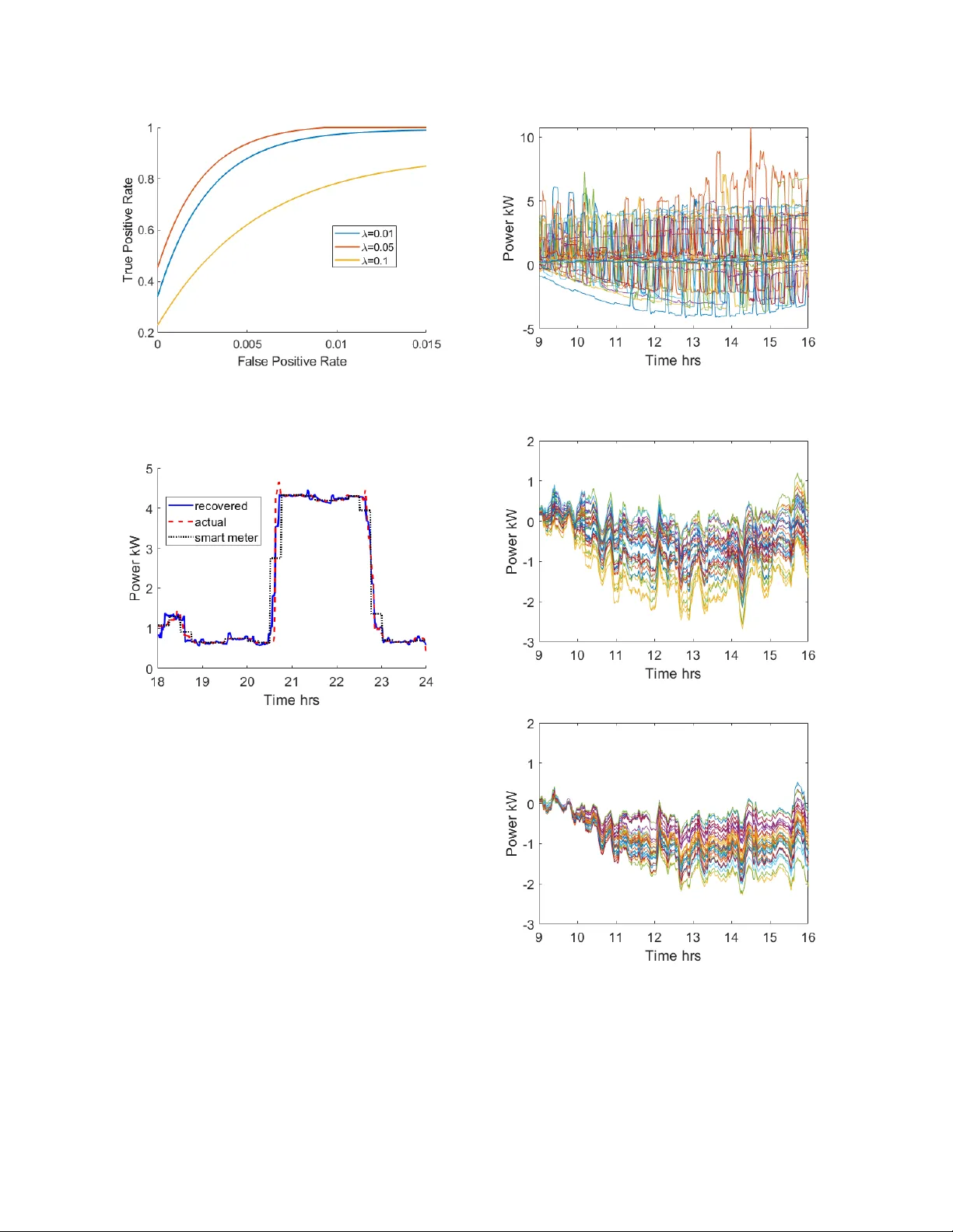
Enhancing the Spatio-T emporal Observ ability of Residential Loads Shanny Lin and Hao Zhu Department of Electrical and Computer Engineering The Univ ersity of T exas at Austin Emails: {shannylin,haozhu}@ute xas.edu Abstract Enhancing the spatio-temporal observability of r esiden- tial loads is crucial for achie ving secure and efficient operations in distribution systems with incr easing pen- etration of distributed ener gy resour ces (DERs). This paper pr esents a joint infer ence fr amework for r esi- dential loads by lever aging the real-time measur ements fr om distribution-le vel sensors. Specifically , smart meter data is available for almost e very load with unfor - tunately low temporal r esolution, while distrib ution syn- chr ophasor data is at very fast rates yet available at limited locations. By combining these two types of data with r espective str engths, the pr oblem is cast as a matrix r ecovery one with much less number of observations than unknowns. T o impr ove the r ecovery performance, we intr oduce two re gularization terms to pr omote a low- rank plus sparse structur e of the load matrix via a dif fer- ence tr ansformation. Accor dingly , the r ecovery pr oblem can be formulated as a con vex optimization one which is efficiently solvable. Numerical tests using r eal r es- idential load data demonstr ate the effectiveness of our pr oposed appr oaches in identifying appliance activities and r ecovering the PV output pr ofiles. 1. Introduction Power distribution systems are known to lack in real-time observ ability , especially for the indi vidual res- idential loads. Limited amount of sensor measurements are av ailable for distribution system monitoring, typi- cally from a fe w line monitors and control devices. Con- sequently , traditional distribution state estimation (DSE) methods [1 – 3] suffer from low estimation accuracy and robustness, and, furthermore, the y fail to pro vide timely visibility of residential loads. T o address this challenge, advanced sensing and communication technologies hav e been increasingly deployed in distribution systems. One type of sensing device is the distrib ution synchrophasor measurement unit (D-PMU) [4]. D-PMUs provide high-quality phasor and power measurements at sub-second sampling rates of a few grid locations. In addition, smart meters are widely installed at e very household to collect the elec- tricity consumption data at intervals of 15 minutes to one hour [5]. These two types of sensors show the trade-off between spatial di versity and temporal resolution. Ubiq- uitously available smart meter data can lose the transient load information due to time averaging, while the high- rate D-PMU data suffers from limited deployment due to high installation costs. Therefore, neither type of sen- sors alone can directly provide the dynamic load profile at each feeder node. Meanwhile, increasing penetration of distributed energy resources (DERs) greatly challenges distribu- tion system management, thereby calling for enhanced spatio-temporal observability of residential loads. F or example, to v alidate the security of electric v ehicle (EV) charging command, one can estimate the start/end time of EV char ging using the change points of the high- rate household load profile [6]. Similarly , the dynamic load profile can also be used to verify residential pho- tov oltaic (PV) systems’ in verter control settings [7]. In addition to that, the real-time information on residential PV outputs is necessary for achie ving effecti ve protec- tion design in distribution systems, as the solar genera- tion lev el can significantly affect the fault current magni- tude therein [8]. Hence, residential load profiles of high spatial and temporal resolutions are crucial for achieving secure and reliable operations in distribution systems. This paper proposes a joint inference frame- work for residential loads by le veraging the respective strengths of D-PMU and smart meter data. T o recover the spatio-temporal load matrix, both the smart meter data and the aggreg ated load measurements provided by D-PMUs are modeled as linear transformations of the load matrix (Sec. 2). T o tackle the identifiability issue therein, we first present two key characteristics of the underlying load matrix. While spatial correlation among load profiles manifests in a low-rank matrix of lower - dimensional representation, the nodal appliance acti vi- ties lead to sparse changes in the matrix ro ws. Accord- ingly , the problem boils down to recovering a low-rank plus sparse matrix, closely related to the robust princi- pal component analysis (RPCA) work; see e.g., [9 – 11]. Note that similar approaches have been popularly used in other applications in power systems such as syn- chrophasor data recov ery [12], load data cleansing [13], and forced oscillation location [14]. Ho wever , our resi- dential load data matrix slightly dif fers from these e xist- ing models as a difference transformation is needed for achieving the lo w-rank plus sparse structure. Similar to earlier approaches, we introduce two conv ex re gu- larization norms to match such structural characteris- tics and to cast the reco very problem as a con vex opti- mization one (Sec. 3). A post-processing procedure is dev eloped to improve the estimation error bias due to the regularization penalty , while the recovery perfor- mance is discussed in relation to RPCA results (Sec. 3.1). Numerical tests using real residential load data demonstrate the effecti veness of our approaches in iden- tifying large appliance activities and recovering the PV outputs (Sec. 4). The presence of periodic HV AC loads has resulted in some performance de gradation, thereby pointing out a future direction of including more div erse types of measurements (voltage/current/reacti ve power) for improv ed recovery performance. Notation: Upper (lower) boldface symbols stand for matrices (vectors); ( · ) T stands for matrix transposi- tion; k · k ∗ denotes the matrix nuclear norm; k · k 1 the L1-norm; | · | the entry-wise absolute v alue; and 1 stands for the all-one vector of appropriate size. 2. System Model Consider a distribution feeder system with residen- tial homes connected at the feeder ends as shown in Fig. 1. The goal is to recover the spatio-temporal active power load matrix P ∈ R N × T where N is the num- ber of load nodes (residential households) and T is the total number of time slots. The temporal resolution of P represents the fastest time-scale of the all measure- ments. This work assumes a minute-lev el time resolu- tion, which can be generalized to e ven faster time-scales such as the second-lev el time resolution of actual D- PMUs [15]. T o recover P , we consider tw o types of measure- ment data, namely the smart meter data for each load node and the aggregated power demand at the feeder head. T ypically , all residential households are equipped with smart meters that collect electricity consumption data at interv als of 15-minutes or one hour [5]. Note that in this work, smart meter data is assumed to be av ailable ev ery 15 minutes by av eraging the corresponding 15 samples in P . For each house, ev ery smart meter mea- surement recorded is the av erage active power consumed Figure 1: Overview of the distr ibution feeder system with multiple load nodes and various types of measurements. ov er the data collection interval. Giv en the 1/15 down- sampling rate, the smart meter data matrix Y ∈ R N × T s with T s = T / 15 is giv en by Y = P A + E Y , (1) where matrix A ∈ R T × T s represents the time a verag- ing operation on P while E Y denotes the measurement noise matrix. At the aggregation location, a D-PMU can collect the total load profile, in addition to voltage/current pha- sors, with fast minute-lev el resolution and high qual- ity . T o simplify the model, we assume that the network losses are omitted from this aggregated measurement. Hence, the total load measurement z ∈ R T by aggre gat- ing ov er all N houses is given by z T = 1 T P + e T z , (2) where e z is the D-PMU measurement noise vector and the all-one v ector 1 sums up all nodal profiles. Note that multiple D-PMUs can be included as well using a gen- eral matrix to replace 1 T . Moreover , although we con- sider a simple aggregation scheme, the model in (2) can be generalized to include feeder losses as well. If the losses are a fixed percentage of the total demand, then one can scale the aggregated load measurement to reflect the consumed power only . The most general solution will be to represent the exact losses using (possibly lin- earized) distribution po wer flow models; see e.g., [16]. Clearly , using the measurements in (1) and (2), the problem of recov ering matrix P is underdetermined. The total number of equations, giv en by (1) and (2), equals to ( N T s + T ) which is much smaller than N T , the number of unknowns. Therefore, we will exploit cer- tain characteristics and special structures of matrix P to achiev e good recovery results. 3. Spatio-T emporal Load Recovery It is well known that load demand curves at the transmission lev el exhibit high correlation among nearby locations, and thus share similar temporal pat- terns . This property has been widely used by load fore- casting and data cleansing works; see e.g., [13, 17–19]. Sev eral factors play a role in leading to this similarity , including weather conditions (i.e. temperature, irradi- ance) and economic conditions (i.e. electricity prices). Although this spatial correlation property is well kno wn to hold for transmission-level loads, we have observed it for distribution-lev el loads as well. Fig. 2(a) plots the load profiles of one winter day for 30 residential houses (15 of which hav e PV panels) located in the same neigh- borhood in Austin, TX. Fig. 2(b) plots the load profile of one sel ected house with PV during a summer day . Com- pared to the winter profiles, the summer one has a high lev el of periodic HV A C loads. These plots hav e been generated from minute-level real data av ailable through the PecanStreet Dataport [20]. It has been observed that there exists a daytime temporal pattern among the 15 houses with PVs, corresponding to a typical daily solar irradiance profile in Austin, TX. Similarly for the 15 houses without PVs, they share the same minimal base loading pattern. Additionally , during the time periods with no solar irradiance, all 30 houses share a similar minimal base-load pattern. Thus, the spatial correlation among minute-level residential loads is mainly due to the PV output and the base loading, not from the usage of electric appliances. W e assume load matrix P has an underlying low-rank component L ∈ R N × T , rows of which are either highly correlated (PVs) or close to zero (no PVs). Note that the load nodes are located within the same feeder (connected to the same D-PMU), and, therefore, in the same neighborhood. This ensures that houses with PVs will exhibit similar solar irradiance pat- terns. The effect of a variable type of houses, including houses not co-located, on the similarity of temporal pat- tern and recovery performance will be inv estigated in future. Interestingly , residential load curves go beyond the temporal similarity of transmission loads as they also include rectangular waveforms which are not syn- chronized across locations. These components reflect the large appliance activities at individual households. For e xample, the visible ones in Fig. 2(a) correspond to the charging ev ents of household electric vehicles (EVs), while the frequency patterns in Fig. 2(b) relate to the summer-time HV A C loads. Generally speaking, these appliance activities still occur infrequently over the course of a day and sho w no strong correlation with other households. Hence, they can be captured by sparse changes in the daily load profiles, represented by an (a) (b) Figure 2: Actual residential load profiles a vailable from the PecanStreet Datapor t [20] for (a) 30 houses on a winter da y and (b) a single house with PVs on a sum- mer da y . additional component S ∈ R N × T in matrix P . This sparse-change characteristic has been exploited by [21] to tackle the identifiability issue when only a subset of loads are metered. Note that S itself may not be sparse but rather piece-wise constant. Hence, the consecu- tiv e dif ferences for each load are sparse, as defined by D n,t = S n,t − S n,t − 1 , ∀ ( n, t ) with S n,t = P t τ =1 D n,τ . Thus, matrix S becomes sparse under the linear transfor- mation giv en by S = DU where U ∈ R T × T is an upper triangular matrix of all ones. This way , the data matrix P can be decomposed into a low-rank matrix augmented by an additional sparse-change matrix such that P = L + S = L + DU . This formulation of P mimics the model used by the frame work of rob ust principal component anal- ysis (RPCA) which decomposes a lar ge data matrix into a low-rank plus sparse from [9]. F or RPCA, the lo w- rank component similarly captures the spatial correla- tion among the ro ws, while the sparse component repre- sents outlier entries that are not correlated across rows. Hence, our data model is slightly different from the RPCA setting. Howe ver , by defining matrix W = U − 1 that can compute the consecutive differences between the columns, we obtain X := PW = ( L + DU ) W = K + D (3) where K : = L W is also of low rank. This is because of the temporal pattern in L in Fig. 2(a) leads to high correlation of the column differences of L as well. Clearly , the transformed matrix X satisfies the lo w-rank plus sparse structure, and its components K and D are related to the measurements in (1)-(2) as Y = ( K + D ) UA + E y , (4a) z T W = 1 T ( K + D ) + e T z W . (4b) Now the problem of recov ering P becomes one of recov ering a low-rank plus sparse matrix. One can intro- duce meaningful regularization terms to promote this structure. The nuclear matrix norm has been widely adopted for low-rank matrix recovery in problems such as matrix completion, subspace learning, and collabo- rativ e filtering; see e.g., [9, 11, 22]. The matrix nuclear norm is defined as the sum of the singular values: k K k ∗ : = min { N ,T } X i =1 σ i ( K ) , (5) where σ i ( · ) denotes the i -th largest singular v alue. It is a con ve x function of the matrix input as sho wn in [23, pg. 637], because it is the dual function of the matrix spectral norm (or , the maximum singular value). T o promote sparse D , one can use the popular L1- norm regularization, as used in the fields of compressed sensing and sparse signal recov ery; see e.g., [24–26]. The L1-norm is defined as the sum of entry-wise abso- lute values, gi ven by k D k 1 : = X n,t | D n,t | . (6) Since the L1-norm is a tight con vex relaxation of the L0 pseudo-norm (the number of nonzero entries), it has been shown to be able to efficiently find the sparse signal representation with performance guarantees. Note that the nuclear norm in (5) can be thought of as the L1-norm of the matrix singular v alues. Therefore, minimizing the nuclear norm can lead to fewer numbers of nonzero sin- gular values, and thus a lo w-rank matrix solution. Using the tw o norms, one can formulate the matrix X recovery problem as min K , D k K k ∗ + λ k D k 1 (7a) sub ject to − ξ y ≤ Y − ( K + D ) UA ≤ ξ y (7b) − ξ z ≤ z T W − 1 T ( K + D ) ≤ ξ z (7c) where λ > 0 is a fixed weight coefficient to balance K and D and parameters ξ y , ξ z > 0 are pre-determined error bounds. W e will discuss the choice of λ in Sec. 3.1. As for the error bounds, they can be set accord- ing to the meter accuracy for each type of measure- ment or ev en to account for potential modeling inac- curacy due to e.g., bad data or feeder losses. If only measurement noise is considered, then the infinity norm based error constraints in (7b)-(7c) correspond to uni- formly distributed noise. This assumption is v alid for practical systems as meter accurac y is specified by the maximum error percentage. One can use different error criteria such as the Frobenius norm for Gaussian dis- tributed noise. Moreover , the error bounds can be dif- ferent for ev ery measurement entry , since they would scale with the actual data due to instrumentation as dis- cussed in Sec. 4. The recovery problem (7) is a con- ve x problem that can be solved by generic con vex opti- mization solvers. The computational complexity may grow fast with the matrix dimension, thereby calling for accelerated solutions such as alternating minimiza- tion [27] or adaptiv e updates using subspace learning approaches [28], which will be explored in the future to dev elop fast algorithms for solving (7). One main issue of the proposed recovery formula- tion (7) is that the L1-norm regularization may penalize the magnitude of nonzero entries of D . Hence, the solu- tion ˆ D tends to be smaller in magnitude than the actual values and is thus biased. W e have observed through numerical studies that the presence of frequent HV A C activities during the summer days could make this issue worse. This is because the periodic HV AC activities could exhibit a certain level of temporal pattern, and thus are partially captured by L . As a result, the output ˆ D from (7) is more likely to suffer from smaller magni- tudes. T o tackle this issue, we will dev elop a post- processing scheme based on the recov ered support of ˆ D from (7). Albeit the magnitude bias, the nonzero entries of D can be accurately identified by solving (7). Hence, one can use the solution ˆ D to obtain the sub- set of nonzero entries in M = { ( n, t ) | | ˆ D n,t | > 0 } . In the numerical tests, we use a small positiv e thresh- old to reflect the numerical accuracy of the zero entries. Using the estimated support in M , one can recast the recov ery problem (7) by neglecting the penalty term on Algorithm 1 Recovering matrices K and D 1: Input: Smart meter data Y and D-PMU data z . 2: Output: Estimated ˆ K and ˆ D 3: Step 1: Solve the problem (7) to obtain the biased estimation ˆ K b and ˆ D b . 4: Step 2: Find the set of nonzero entries M := { ( n, t ) | | ˆ D n,t | > 0 } . 5: Step 3: Solve the problem (8) using M to obtain the updated estimates ˆ K and ˆ D . D . Instead, an additional constraint can be introduced to directly set all other entries not in M to be zero. W ith the gi ven M , the post-processing problem is formulated as min K , D k K k ∗ (8a) sub ject to D n,t = 0 , ∀ ( n, t ) 6∈ M (8b) − ξ y ≤ Y − ( K + D ) UA ≤ ξ y (8c) − ξ z ≤ z T W − 1 T ( K + D ) ≤ ξ z . (8d) This way , the nonzero entries of D can be better esti- mated. The full matrix recovery algorithm including this post-processing step is tabulated in Algorithm 1. 3.1 Recovery Perf ormance This subsection discusses the reco very guarantees that could be achiev ed by problem (7), as related to the theoretical results from the RPCA work; see e.g., [9 – 11]. As mentioned earlier , the general RPCA frame- work deals with the similar low rank plus sparse matrix form, but assumes the full (or partial) observability of the full matrix itself. Hence, the theoretical results therein is not directly applicable to our problem setting where the unknown matrix is observed with dimension- ality reduction of both column- and ro w-space [cf. (4)], at the ratios of T /T s and N / 1 , respectiv ely . Nonethe- less, the RPCA results can still provide insightful intu- itions regarding the recovery conditions and the param- eter settings in our framew ork. Certain conditions on K and D are required in order to achieve accurate RPCA results [9, 28, 29]. Loosely speaking, the low rank component K cannot be sparse and the sparse component D cannot be of low rank. For K , the column space spanned by either its left or right singular vectors needs to have low to almost zero in coherency with the identity matrix, thereby ensuring the singular vectors are not sparse. This implies that the temporal pattern of load profiles cannot be sparse itself. Meanwhile, for the sparse component D , the location of its non-zero entries should be random with no peri- odic or correlated patterns. The randomness condition would promote D to be, ideally , full rank, while a non- periodic sparse pattern would make sure no frequency- induced low-rank component exists in D . As it will soon become clear in Section 4, the non-periodic condition is v ery important in the analysis of summer-time data, where frequent HV A C acti vities could be problematic in recov ering the low-rank and sparse components of the load matrix. The other insight provided by the RPCA work is the choice of weight λ , used to balance the low-rank and sparse components. As mentioned in [9, 11], the λ value should be chosen according to the matrix dimension, as O (1 / √ T ) if the dimension T  N . This setting can effecti vely balance the scaling of the two norms with respect to T , at around √ T and T , respectiv ely . It will be used by numerical tests in Section 4. 4. Simulation Results This section presents the numerical results of recov ering P obtained by solving problem (7) and using Algorithm 1 on a winter and summer data set respec- tiv ely . For the winter data set, it turns out the solution to (7) is sufficiently good as there is no periodic HV A C activity that could potentially lead to biased D . Ho w- ev er , for the summer data set with high lev el of HV A C activities, the post-processing step in Algorithm 1 turns out to be useful as it improves the separation of the cor- related PV profiles from the sparse appliance ev ents. The ground-truth data P is obtained from the PecanStreet’ s Dataport [20] for the 30 residential homes shown in Fig. 2(a) for one winter day and similarly for one summer day . The active power demand data is at minute-lev el resolution. Only half of the houses hav e PVs installed and all the houses are located in the same neighborhood (Mueller, Austin). Only 6 houses hav e EV charging ev ents. Based on P , we syntheti- cally generate the measurements in (1)-(2) by adding random noise. Additionally , we assume that the smart meters record at 15 minute intervals. Using the Ameri- can National Standard Institute (ANSI) C12.20 Standard [30], we assume the smart meters installed at each resi- dential home are rated at ± 0.2% error accuracy . Accord- ingly , the entries of E y are independently dra wn from a uniform distribution based on this accuracy . As for the fast aggregated measurement z , we follow from the D-PMU data-sheet [15], where the ± 0.01% total vector error of the phasor measurement leads to acti ve power measurement error within ± 0.02%. Hence, the entries of e z are drawn from independent uniform distributions using the ± 0.02% accuracy . T o solve the con vex problem (7), we need to deter- mine the value of the tuning parameter λ and the error bounds ξ y and ξ z . For all of the following test cases, a (a) (b) Figure 3: Comparison between (a) the actual residential load profiles and (b) the recov ered ˆ P f or the winter day- time loads in test case 1. value of 0.05 was used for λ . This v alue is chosen based on O (1 / √ T ) (cf. Sec. 3.1) and it has produced consis- tently good reco very results. The error bounds ξ y and ξ z are determined based upon the added noise lev el to the synthetic data, where ξ y is set to be 0 . 2% | Y | while ξ z is 0 . 02% | z | T | W | . T o implement the con vex problems (7) and (8), we use the generic conv ex solver CVX [31] in the MA TLAB R  R2018a simulator, on a laptop with Intel R  Core TM i7 CPU @ 2.10 GHz and 8 GB of RAM. Under this setting, the computational time for each problem is pretty reasonable, taking around 5-10 minutes to process a total of 7 hours of load data. W e will de velop acceler- ated solutions as mentioned in Sec. 3 in the future. 1) T est Case 1 on winter day-time data: W e first test the winter data set for the day-time period from 9:00- 16:00 to recover the solar irradiance pattern. Fig. 3(b) shows the reco vered ˆ P obtained by (7) which matches (a) (b) (c) Figure 4: Recov ered winter solar irradiance pattern in test case 1: (a) the estimated ˆ L for all 30 houses and (b) its first right singular vector , compared with with (c) the ground-truth PV output data for the 15 houses with PVs . well with the ground-truth data in Fig. 3(a). Although ˆ P is unable to capture the fast transients in the ground- Figure 5: Receiving operating curve (fitted by an expo- nential function) for test case 2 showing the true positives versus f alse positives f or detecting EV ev ents. Figure 6: Recov ered load data for one residential home with an EV charging e vent in test case 2. truth data, it has included the major changes of dynamic load profiles such as the PV variations. T o better illus- trate the PV output recov ery results, Fig. 4 plots the estimated ˆ L and compares it with the ground truth data. Clearly , the estimated ˆ L in Fig. 4(a) is of v ery lo w rank, with its first right singular vector in Fig. 4(b). As men- tioned in Sec. 3 the temporal pattern is mainly due to the PV outputs. Although ˆ L does not recover the actual ground-truth PV output, its first right singular v ector has captured the main temporal pattern and can indicate the recov ered PV output. It indeed matches well with the solar irradiance pattern present in the ground-truth PV outputs in Fig. 4(c). Since the winter data set does not contain HV A C acti vities, the low-rank component ˆ L can be ideally separated from the sparse changes and it con- tains mainly the solar irradiance pattern. 2) T est Case 2 on winter night-time data: W e fur- Figure 7: Ground-truth load profile for test case 3. (a) (b) Figure 8: Recov ered ˆ L from (a) the solution to (7) and (b) Algorithm 1 in test case 3. ther test the winter data set for the night time period from 18:00-24:00 to demonstrate the capability of recovered (a) (b) Figure 9: Recovered solar irradiance patter n: (a) the first right singular vector of the estimated ˆ L using Algorithm 1, and (b) the PV -only output data. ˆ P in identifying EV e vents. Fig. 5 plots the recei ving operating curve (ROC) of detected EV start/stop charg- ing events as compared to the ground truth for three λ values. Note that each R OC has been fitted with an expo- nential function. For each λ , the R OC is created by vary- ing the detection threshold (as a percentage of EV power rating). As the EVs have lar ger power ratings than other appliances, the false positi ve (or false alarm) rate is v ery small. Fig. 5 corroborates our recovery method’ s per - formance in EV identification, as all ROCs are close to perfect detection (top left corner of the plane). Addi- tionally , the value λ = 0 . 05 , as chosen for all our tests cases, is very competiti ve among the three. One resi- dential load is selected to demonstrate the recov ery of an EV charging event occurring at around 20:30-23:00, as shown in Fig. 6. Compared to the smart meter mea- surements which fail to indicate the exact EV charging start/finish time, our estimated profile can well match (a) (b) (c) Figure 10: Selected residential load profiles in test case 3 for a house with (a) no HV A C activity , (b) per iodic HV AC activity , and (c) one EV charging ev ent from 12:00-14:30. the actual minute-lev el profile. 3) T est Case 3 on summer day-time data: Lastly , we test the summer data set for the day-time period from 9:00-16:00 to demonstrate the impact of frequent HV A C activities. As shown in Fig. 2(b), there is a high lev el of HV A C acti vity in the summer data. The periodicity of the HV A C ev ents would also manifest in a low-rankness of the load matrix, which would make it challenging to keep it solely in the sparse component D . T o help improv e the summer data recov ery , we apply the post- processing step described in Algorithm 1. Fig. 7 and Fig. 8 plot respectively the ground-truth load profile and the recovered ˆ L using both the solution from (7) and Algorithm 1. Although the two estimates of ˆ L look very similar , the post-processing step has shown to improv e the recov ery of solar irradiance profile. With- out the post-processing step, there are some large, peri- odic transients present in the estimated ˆ L , as shown by Fig. 8(a). The transients are mainly due to the peri- odic HV A C activities and the penalty on the magnitude of ˆ D in the objective of (7). After re-estimating ˆ L and ˆ D using (8), Algorithm 1 is able to improv e the reco very of the magnitude of the entries in the estimated support set M . Accordingly , Fig. 8(b) shows that the lar ge tran- sients hav e been reduced in ˆ L . T o better show the recov- ery improvement in the PV profiles, Fig. 9 compares the the first right singular vector of the post-processed ˆ L to the ground-truth PV output data. The parabolic trend in the residential PV output data is well recovered by the low-rank component. Compared to the winter data results, the recovered ˆ L here is affected by the periodic HV A C acti vities, and, therefore, exhibits some oscilla- tion patterns of around 30-minute interv als as opposed to the smoother trend in the actual PV profiles. Fig. 10 sho ws the recovered residential load pro- files for three selected houses. The recovered load pro- files captures the trend in the actual profiles. Howe ver , they are unable to match most of the fast HV A C ev ents. Upon closer observation, we find out that the estimated profiles follow the smart meter data more often in the presence of periodic changes, as shown in Fig. 10(b)- (c). Nonetheless, the proposed method can well cap- ture the significant amount of change in the load pro- files, such as EV charging as sho wn in Fig. 10(c). Intu- itiv ely speaking, the performance degradation in recov- ering the summer time data is fundamentally due to the lack of observability in our system set-up. As there are increasing amount of transient events in the underlying load matrix, we need to use more measurements to be able to keep up with the unknown information. In other words, a single aggre gated load profile pro vides insuf- ficient amount of spatial diversity that is present in the unknown load data. Therefore, we should e xplore var- ious types of data (v oltage/current/reactive po wer) that D-PMUs can provide in addition to increasing the num- ber of D-PMUs. This would require the incorporation of distribution feeder modeling and it is currently pursued to generalize the proposed load recov ery framework. 5. Conclusions This paper presents a matrix recov ery algorithm to enhance the spatio-temporal observability of residential loads by jointly utilizing both the smart meter and D- PMU data. Using the appropriate norm re gularization, this problem is cast as a con vex optimization one to pro- mote the underlying low-rank and sparse change charac- teristics of the unkno wn load matrix. A post-processing procedure is developed as well to mitigate the estimation bias due to the regularization penalty . Numerical test results using real residential load data demonstrate that the reco very algorithm can ef fectively recover appliance activities and the PV output profiles. Ho wev er, the pres- ence of periodic HV A C loads would lead to some per - formance de gradation in correctly identifying the sparse changes. W e are currently e xploring the use of v arious types of D-PMU data, in addition to increased number of D- PMUs, for improv ed recovery performance. Further- more, we plan to in vestigate accelerated and online solu- tion methods that can be implemented efficiently and in real-time. Acknowledgments This work has been supported by the NSF Grant ECCS-1802319 and the DOE CEDS program. References [1] A. Primadianto and C.-N. Lu, “A Revie w on Dis- tribution System State Estimation, ” IEEE T ransac- tions on P ower Systems , vol. 32, no. 5, pp. 3875– 3883, Sept. 2017. [2] C. Lu, J. H. T eng, and W .-H. E. Liu, “Distribu- tion system state estimation, ” IEEE T ransactions on P ower Systems , vol. 10, no. 1, pp. 229–240, Feb . 1995. [3] M. E. Baran and A. W . Kelle y , “State estimation for real-time monitoring of distribution systems, ” IEEE T ransactions on P ower Systems , vol. 9, no. 3, pp. 1601–1609, Aug. 1994. [4] A. von Meier , D. Culler, A. McEachern, and R. Arghandeh, “Micro-Synchrophasors for Distri- bution Systems, ” IEEE PES Inno vative Smart Grid T ec h. Conf. , Feb . 2014. [5] “Advanced Metering Infrastructure and Customer Systems, ” U.S. Department of Energy , Sept. 2016. [Online]. A vailable: https://www .energy .gov/sites/prod/files/2016/12/ f34/AMI%20Summary%20Report_09- 26- 16.pdf [6] C. Niddodi, S. Lin, S. Mohan, and H. Zhu, “Secure integration of electric vehicles with the power grid, ” arXiv pr eprint arXiv:1905.01035 , 2019. [7] N. Jacobs, S. Hossain-McKenzei, D. Jose, D. Saleem, C. Lai, P . Cordeira, A. Hasandka, M. Martin, and C. Howerter , “ Analysis of System and Interoperability Impact from Securing Com- munications for Distributed Energy Resources, ” 2019 IEEE P ower and Ener gy Conference at Illi- nois (PECI) , 2019. [8] X. Zheng, X. Geng, L. Xie, D. Duan, L. Y ang, and S. Cui, “A SVM-based setting of protection relays in distrib ution systems, ” 2018 IEEE T e xas P ower and Ener gy Conference (TPEC) , 2018. [9] E. J. Candès, X. Li, Y . Ma, and J. Wright, “Robust principal component analysis?” Journal of the A CM (JA CM) , vol. 58, no. 3, p. 11, 2011. [10] H. Xu, C. Caramanis, and S. Sanghavi, “Robust PCA via Outlier Pursuit, ” IEEE T ransactions on Information Theory , v ol. 58, no. 5, pp. 3047–3064, 2012. [11] J. Wright, A. Ganesh, S. Rao, Y . Peng, and Y . Ma, “Rob ust principal component analysis: Exact recovery of corrupted low-rank matrices via con vex optimization, ” in Advances in Neural Infor- mation Pr ocessing Systems 22 , 2009, pp. 2080– 2088. [12] P . Gao, M. W ang, S. G. Ghiocel, J. H. Chow , B. Fardanesh, and G. Stefopoulos, “Missing Data Recov ery by Exploiting Lo w-dimensionality in Power Systems Synchrophasor Measurements, ” IEEE T rans. P ower Systems , vol. 31, no. 2, pp. 1006–1013, Mar . 2016. [13] G. Mateos and G. B. Giannakis, “Load Curve Data Cleansing and Imputation V ia Sparsity and Low Rank, ” IEEE T rans. on Smart Grid , vol. 4, no. 4, Dec. 2013. [14] T . Huang, N. M. Freris, P . R. Kumar , and L. Xie, “Localization of forced oscillations in the power grid under resonance conditions, ” 2018 52nd Annual Confer ence on Information Sciences and Systems (CISS) , 2018. [15] “microPMU Data Sheet, ” Power Standards Lab, 2018. [Online]. A vailable: https://www . powerstandards.com/do wnload- center/micropmu/ [16] A. Bernstein, C. W ang, E. Dall’Anese, J.-Y . Le Boudec, and C. Zhao, “Load flow in multiphase distribution networks: Existence, uniqueness, non- singularity and linear models, ” IEEE T ransactions on P ower Systems , v ol. 33, no. 6, pp. 5832–5843, 2018. [17] P . W ang, B. Liu, and T . Hong, “Electric load fore- casting with recency effect: A big data approach, ” International Journal of F or ecasting , vol. 32, no. 3, pp. 585–597, 2016. [18] S.-J. Kim and G. B. Giannakis, “Load Forecast- ing via Low Rank Plus Sparse Matrix Factoriza- tion, ” 2013 Asilomar Confer ence on Signals, Sys- tems and Computers , Nov . 2013. [19] J.-B. Fiot and F . Dinuzzo, “Electricity Demand Forecasting by Multi-T ask Learning, ” IEEE T rans. on Smart Grid , vol. 9, no. 2, pp. 544–551, Mar . 2018. [20] “PecanStreet Dataport, ” PecanStreet Inc. [Online]. A vailable: https://dataport.cloud/ [21] S. Bhela, V . Kekatos, and S. V eerachachaneni, “Enhancing Observ ability in Distrib ution Grids Using Smart Meter Data, ” IEEE T ransactions on Smart Grid , vol. 9, no. 6, No v . 2018. [22] B. Recht, M. Fazel, and P . A. Parrilo, “Guaranteed minimum-rank solutions of linear matrix equations via nuclear norm minimization, ” SIAM Review , vol. 52, no. 3, pp. 471–501, 2010. [23] S. Bo yd and L. V andenber ghe, Conve x Optimiza- tion , 1st ed. New Y ork, NY : Cambridge Uni ver - sity Press, 2004. [24] S. S. Chen, D. L. Donoho, and M. A. Saunders, “ Atomic decomposition by basis pursuit, ” SIAM r eview , v ol. 43, no. 1, pp. 129–159, 2001. [25] E. Candes and T . T ao, “Near-optimal signal recov- ery from random projections: Uni versal encod- ing strategies?” IEEE T ransactions on Information Theory , vol. 12, no. 52, pp. 5406–5425, 2006. [26] D. L. Donoho, “For Most Large Underdetermined Systems of Linear Equations of Minimal L1-norm Solution Is Also The Sparsest Solution, ” Comm- nunications on Pure and Applied Mathematics , vol. 59, no. 6, pp. 797–829, 2006. [27] Z. Lin, M. Chen, and Y . Ma, “The augmented lagrange multiplier method for exact recovery of corrupted low-rank matrices, ” arXiv pr eprint arXiv:1009.5055 , 2010. [28] N. V aswani, T . Bouwmans, S. Ja ved, and P . Narayanamurthy , “Robust subspace learning: Robust pca, robust subspace tracking, and robust subspace recov ery , ” IEEE Signal Pr ocessing Mag- azine , vol. 35, no. 4, pp. 32–55, 2018. [29] V . Chandrasekaran, S. Sanghavi, P . A. Parrilo, and A. S. Willsk y , “Rank-Sparsity Incoherence for Matrix Decomposition, ” SIAM Journal on Opti- mization , vol. 21, no. 2, pp. 572–596, 2011. [30] “ANSI C12.20-2015-Electricity Meters-0.1, 0.2, and 0.5 Accurac y Classes, ” Amer- ican National Standards Institute, 2015. [Online]. A vailable: https://blog.ansi.or g/2017/05/ ansi- c1220- 2015- electricity- meters- accuracy- classes/ [31] “CVX: Matlab Software for Disciplined Con vex Programming, ” CVX Research, 2018. [Online]. A vailable: http://cvxr .com/cvx/