A Fast and Robust Algorithm for Orientation Estimation using Inertial Sensors

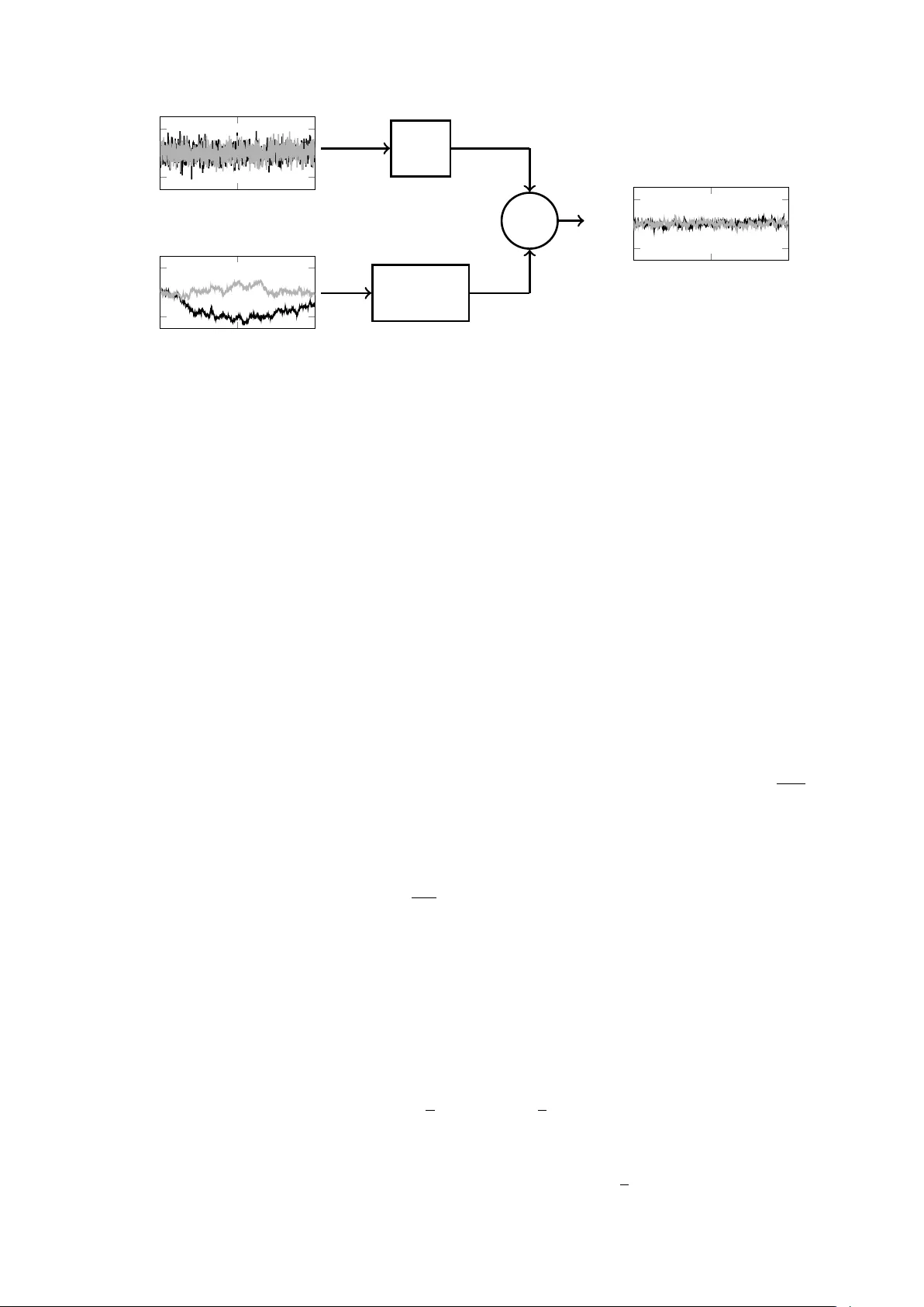
A F ast and Robust Algorithm for Orien tation Estimation using Inertial Sensors Manon Kok ? and Thomas B. Sc h¨ on ?? ? Delft Cen ter for Systems and Control, Delft Univ ersit y of T echnology , the Netherlands, e-mail: m.k ok-1@tudelft.nl ?? Departmen t of Information T echnology , Uppsala Univ ersit y , Sweden, e-mail: thomas.sc hon@it.uu.se • Please cite this v ersion: Manon Kok and Thomas B. Sc h¨ on, “A F ast and Robust Algorithm for Orientation Estimation using Inertial Sensors”, IEEE Signal Pro cessing Le tters, 2019. DOI: 10.1109/LSP .2019.2943995 Abstract W e present a nov el algorithm for online, real-time orien tation estimation. Our algorithm integrates gyroscop e data and corrects the resulting orien tation estimate for in tegration drift using accelerom- eter and magnetometer data. This correction is computed, at eac h time instance, using a single gra- dien t descent step with fixed step length. This fixed step length results in robustness against mo del errors, e.g. caused by large accelerations or by short-term magnetic field disturbances, whic h w e n umerically illustrate using Monte Carlo sim ulations. Our algorithm estimates a three-dimensional up date to the orientation rather than the entire orientation itself. This reduces the computational complexit y b y appro ximately 1/3 with resp ect to the state of the art. It also improv es the quality of the resulting estimates, specifically when the orien tation corrections are large. W e illustrate the efficacy of the algorithm using exp erimental data. Keywor ds: Orien tation estimation, inertial sensors, complemen tary filter, m ultiplicativ e extended Kalman filter. 1 In tro duction Orien tation estimation using inertial and magnetometer measurements is by now a w ell-studied problem with applications in e.g. h uman motion analysis [1, 2] and rob otics [3, 4]. In recent y ears, there has b een an increasing demand for algorithms that are computationally inexp ensive and that can estimate orientation in real-time on a microprocessor, e.g. illustrated by the wide-spread use of the techniques from [5, 6]. These algorithms op en up for real-time human motion analysis [7, 8] and control of rob ots [4, 9]. In this w ork w e present a nov el computationally efficient algorithm for orientation estimation. Our algorithm’s robustness against inaccuracies in the accelerometer and magnetometer measuremen t mo dels adds to its practical usefulness. There exists a v ast range of orien tation estimation algorithms. Their differences lie b oth in the estimation method and in the parametrisation of the orientation. F or example, b oth [5, 6] and the extended Kalman filter (EKF) presen ted in [10] estimate the orientation parametrised as a unit quater- nion. Normalisation of these unit quaternions is necessary for the estimates to remain v alid orientations. This normalisation in tro duces errors especially when large updates to the estimates are made, for in- stance due to low sampling rates or large initialisation errors [11, 12]. Alternativ ely , algorithms can estimate orientation deviation from a linearisation p oin t, see e.g. [13, 14]. An example is provided b y the m ultiplicative EKF (MEKF) that parametrises the orientation deviation in terms of a rotation vector (axis-angle) [12, 15, 16]. A similar approac h is often used in rob otics [17 – 21]. This form ulation av oids the issues with quaternion normalisation while at the same time reducing the state dimension. In our algorithm, we make similar design choices as the widely used filter published by Madgwick et al. [5, 6]. Because of this, our filter inherits its desirable prop erties such as easy tuning and accurate estimates also in the presence of model errors. How ever, since w e estimate the orientation in terms of an orien tation deviation parametrised using a rotation vector, our filter reduces the computational com- plexit y b y approximately 1/3 and obtains more accurate estimates when large up dates to the estimates are made. 2 Bac kground on sensor mo dels Our algorithm mak es use of standard sensor mo dels for orientation estimation, hence ensuring the wide applicabilit y of our method. First of all, w e model the gyroscop e measuremen ts y ω ,t as y ω ,t = ω t + e ω ,t , (1) where ω t denotes the angular v elocity and e ω ,t the measuremen t noise. Note that the sensor model (1) can optionally b e extended with a gyroscop e bias. W e assume that the sensor’s acceleration a n is appro ximately zero and that the accelerometer therefore only measures the Earth’s gra vit y g n . The sup erscript n explicitly indicates that the vector is expressed in the navigation frame n , whic h is aligned with Earths gravit y and the local (Earth’s) magnetic field. The accele rometer measurements y a ,t are hence mo delled as y a ,t = R ( q bn t ) ( a n − g n ) + e a ,t ≈ − R ( q bn t ) g n + e a ,t . (2) W e represent the orientation at time t using a unit quaternion denoted by q nb t . The sup erscript nb indicates that the quaternion represents the rotation from the b o dy frame b , which is aligned with the sensor axes, to the navigation frame n . The op eration R ( q nb t ) conv erts the quaternion to a rotation matrix. The rev erse orien tation used in (2) is given by R ( q nb t ) = ( R ( q bn t )) T . Due to the fact that the Earth’s gravit y dep ends on the sensor’s lo cation and since the unit in whic h the sensor expresses the acceleration v aries, we assume that y a ,t has unit norm and define g n =  0 0 1  T . T o this end, we prepro cess the accelerometer measuremen ts b efore using them in the measuremen t mo del (2). W e assume that the magnetometer measures a lo cal, constant (Earth’s) magnetic field m n . The magnetometer m easuremen ts y m ,t are therefore mo delled as y m ,t = R ( q bn t ) m n + e m ,t . (3) Because the unit in whic h the sensor expresses the magnetic field measurement v aries, we normalise the magnetometer measurements b efore using them in the mo del (3). F urthermore, w e assume that m n =  cos δ 0 − sin δ  T , where δ is the lo cal dip angle. Alternatively , there also exist methods to estimate the lo cal magnetic field from data, see e.g. [5]. 1 G ( s ) 1  G ( s ) ⌃ + + 0 500 1000  2 0 2 T ime [s] Inclination [  ] 0 500 1000  2 0 2 T ime [s] Inclination [  ] 0 500 1000  2 0 2 T ime [s] Inclination [  ] Figure 1: Illustration of the complementary filter for inclination estimation using simulated data. The inclination (roll in black, pitch in grey) from the accelerometer (top left) is lo w-pass filtered while the inclination from the gyroscop e (b ottom left) is high-pass filtered to obtain the resulting inclination estimate (right). Note that the noise terms e a ,t and e m ,t consist of b oth the sensor noise as w ell as mo del errors. These mo del errors are for instance due to non-zero acceleration or due to the presence of ferromagnetic material in the vicinity of the sensor. 3 F ast and Robust Orien tation Estimation Assuming well-calibrated sensors and a kno wn initial orien tation, it is p ossible to estimate the sensor orien tation based only on the gyroscop e measurements. This estimate, which w e denote by q nb ω , is accurate on a short time scale but drifts o v er longer time horizons. On the other hand, the orien tation can be estimated using the accelerometer and magnetometer measurements. This estimate, denoted b y q nb am , is less accurate than q nb ω on a short time scale but does not drift. These complementary prop erties can b e exploited using a c omplementary filter in which q nb am is low-pass filtered while q nb ω is high-pass filtered [22, 23]. This can b e written as ˆ Q nb ( s ) = G ( s ) Q nb am ( s ) + (1 − G ( s )) Q nb ω ( s ) , (4) where s denotes the Laplace v ariable. F urthermore, the transfer function G ( s ) is given by G ( s ) = 1 as +1 , Q nb ( s ) denotes the orientation q nb in the Laplace domain and ˆ q nb is the resulting filtered orientation. This pro cess is visualised in Figure 1. Discretising (4) using bac kw ard Euler gives ˆ q nb t = (1 − γ t ) q nb am ,t + γ t  ˆ q nb t − 1 + T ω q ,t  , (5) where T denotes the sampling time, γ t = a a + T and ω q ,t represen ts the angular v elo cit y expressed in terms of a quaternion. A t first glance, (5) might cause concern because ˆ q nb t will not b e a v alid rotation since this quaternion is no longer normalised. It will, how ever, b ecome clear in the remainder of this section that the deviation from the unit norm will b e small due to the high sampling rates of the sensors. This deviation can b e resolved by normalising ˆ q nb t . Although this leads to minor inaccuracies, it is fairly common practice in many orientation estimation algorithms, see [12] and references therein. 3.1 Orien tation from gyroscop e measuremen ts The angular v elo cit y measured b y the gyroscop e can be used to mo del the dynamics of the orien tation as [12, 24] q nb t = q nb t − 1  exp q  T 2 y ω ,t  ≈ q nb t − 1 + T 2 S ( q nb t − 1 ) y ω ,t , (6) where  denotes the quaternion product and exp q denotes the quaternion version of the v ector defined as exp q ( y ) =  cos α v T sin α  T , α = k y k 2 , v = y α . (7) 2 F urthermore, for q =  q 0 q 1 q 2 q 3  T =  q 0 q T v  T , S ( q ) =  − q v q 0 I 3 − [ q v × ]  , (8) where [ · × ] denotes the matrix cross product and I 3 denotes the iden tity matrix of size 3. Comparing (5) and (6), w e ha v e that the angular velocity expressed in terms of a quaternion is given by ω q ,t = 1 2 S ( ˆ q nb t − 1 ) y ω ,t . (9) 3.2 Orien tation from accelerometer and magnetometer Estimating the orien tation from accelerometer and magnetometer measurements is a widely kno wn prob- lem, see e.g. [25, 26]. It can be form ulated as an optimisation problem min η t V ( η t ) = min η t 1 2 k y a ,t + (exp R ( η t )) T R ( ˜ q bn t ) g n k 2 2 + 1 2 k y m ,t − (exp R ( η t )) T R ( ˜ q bn t ) m n k 2 2 , (10) where k · k 2 denotes the tw o-norm. In (10) w e use the measurement mo dels (2) and (3) but write the orien tation in terms of a linearisation p oint and an asso ciated deviation as R ( q nb t ) = R ( ˜ q nb t ) exp R ( η t ) , (11a) exp R ( η t ) = I 3 + sin α [ v × ] + (1 − cos α ) [ v × ] 2 ≈ I 3 + [ η t × ] , (11b) where the approximation in (11b) assumes small η t . Rewriting the problem in this w a y allo ws us to optimise ov er an orientation deviation parametrised in terms of a rotation v ector [12, 27], rather than optimising o ver a unit quaternion. W e therefore a v oid issues with quaternion normalisation. F urther- more, the n umber of optimisation v ariables reduces from four to three. Our approach draws inspiration from the m ultiplicativ e extended Kalman filter (MEKF) [12, 15, 16] and from approac hes within the field of rob otics [17–21]. Inspired b y [5, 6], instead of solving (10) for each time step, we p erform only a single gradien t descen t iteration. This results in a significan t computational sp eed-up and b ecause of the high sampling rates of the sensors, the corrections that need to be made are t ypically minor and the estimates will conv erge o ver time. Linearising V ( η t ) from (10) around ˜ q bn t = ˆ q bn t − 1 , η t = 0 using (11b), the gradient descent step is given by ˆ η t = − µ t ∇ V ( η t ) , (12a) ∇ V ( η t ) = − [ R ( ˆ q bn t − 1 ) g n × ]  y a ,t + R ( ˆ q bn t − 1 ) g n  + [ R ( ˆ q bn t − 1 ) m n × ]  y m ,t − R ( ˆ q bn t − 1 ) m n  , (12b) where µ t is the gradien t descent step length. The estimate η t can subsequently b e used to compute q nb am ,t from (5) as q nb am ,t = ˆ q nb t − 1  exp q  1 2 ˆ η t  ≈ ˆ q nb t − 1 + 1 2 S ( ˆ q nb t − 1 ) ˆ η t . (13) 3.3 Resulting algorithm Inserting (13) and (9) into (5), w e obtain ˆ q nb t = ˆ q nb t − 1 + 1 2 S ( ˆ q nb t − 1 ) ( γ t T y ω ,t − µ t (1 − γ t ) ∇ V ( η t )) . (14) It no w remains to c ho ose γ t and µ t . Similarly to [5], we choose γ t ≈ 1. In other w ords, we mainly rely on the in tegration of the gyroscop e measuremen ts, but use the accelerometer and magnetometer measuremen ts to correct for the integration drift illustrated in Fig. 1. This choice is motiv ated b y the fact that the orien tation estimates obtained from the accelerometer and the magnetometer are typically more noisy than those obtained using the gyroscop e measurements (see Fig. 1). F urthermore, the accelerometer and the magnetometer measurement models (2) and (3) are often violated due to acceleration of the sensor or the presence of magnetic disturbances. Similarly to [5], w e c ho ose the scaling factor of the gradient descent direction, µ t (1 − γ t ), equal to β T k∇ V ( η t ) k . W e will in Section 4 illustrate that scaling the step with the norm k∇ V ( η t ) k results in an 3 Alg. 1: F ast and Robust Orientation Estimation Input: Gyroscop e measuremen ts y ω ,t , normalised accelerometer and magnetometer measuremen ts y a ,t and y m ,t , sampling time T , tuning parameter β and the orientation estimate at the previous time instance ˆ q nb t − 1 . Output: Orien tation estimate ˆ q nb t . 1: Compute ∇ V ( η t ) from (12b) using y a ,t , y m ,t and ˆ q nb t − 1 . 2: Obtain the up dated orientation estimate ˆ q nb t from (15) using ∇ V ( η t ), β , y ω ,t , T , ˆ q nb t − 1 and S ( q ) from (8). algorithm that is quite robust against violations of the accelerometer and magnetometer measuremen t mo dels. The c hoice of β dep ends on the amount of drift exp ected from in tegration of the gyroscope noise. In the case of Gaussian noise on the gyroscop e data, e ω ,t ∼ N (0 , σ 2 ω ), integration of the gyroscop e measuremen ts in one dimension results in an in tegration drift distributed as T e ω ,t ∼ N (0 , T 2 σ 2 ω ). Using the fact that the gyroscop e measurements are a three-dimensional v ector and are integrated according to (6), the standard deviation of the integration drift on the unit quaternion is given by √ 3 σ ω T . This is therefore a reasonable choice for β T resulting in a go o d compromise. The resulting filter equations can no w be written as ˆ q nb t ≈ ˆ q nb t − 1 + T 2 S ( ˆ q nb t − 1 ) ˆ ω t , (15a) ˆ ω t = y ω ,t − β ∇ V ( η t ) k∇ V ( η t ) k , (15b) and the resulting solution is summarised in Alg. 1. As can b e seen in (15), we directly estimate the angular v elo city which is subsequently used to up date the orientation. This has close connections to the approac hes discussed in [28, 29]. 4 Numerical Illustrations In this section we n umerically illustrate the properties of Alg. 1 and compare them to the filter from [5, 6] and to an MEKF implemented as describ ed in [12]. T o this end, we run 100 Mon te Carlo simulations, eac h consisting of 8000 samples during whic h the sensor is first stationary for 200 samples and then consecutiv ely rotates 360 degrees around each axis in 200 samples p er rotation axis. This mov emen t is rep eated 10 times. The sampling time is set to 10 Hz. F or ease of in terpretation, we decouple the magnetometer and accelerometer information by assuming that the measurements are collected on the equator, i.e. the dip angle δ is zero and hence m n =  1 0 0  T . 4.1 Computational complexity One of the widely known b enefits of the filter from [5, 6] is its lo w computational complexity . More sp ecifically , the filter uses only 218 arithmetic op erations p er filter iteration. Instead of directly estimating the orientation parametrised as a unit quaternion, we estimate the angular velocity as describ ed in (15), effectiv ely reducing the state dimension from 4 to 3. This reduces the n umber of arithmetic op erations p er filter iteration to 140, a reduction of 36%. In T able 1 we show the av erage computational time per filter iteration in our sim ulations for a Matlab implementation run on a 3.1 GHz In tel Core i5 pro cessor. As can b e seen, Alg. 1 is indeed 36% faster than the filter from [5, 6]. Note that our MEKF implementation has not b een optimised for computational sp eed but is kno wn to be slo w er than b oth other filters. 4.2 Gaussian noise with known c haracteristics W e first consider an idealised case where the measurement noises are Gaussian with known cov ariances and the initial sensor orientation is kno wn. More sp ecifically , we set the standard deviation of the gyroscop e noise to σ ω = 5 π 180 rad/s, and that of the normalised accelerometer and magnetometer noise to σ a = σ m = 0 . 01. F or Alg. 1 we c ho ose β as explained in Section 3. W e tune the filter from [5, 6] similarly (setting the tuning parameter in that filter to q 3 4 σ ω ). Note that different v alues of these parameters did not impro ve the p erformance of the algorithms. The MEKF is exp ected to outp erform the other tw o algorithms since the up date equation of an EKF is t ypically closer to optimal than the update equation based on a normalised gradien t descent step. The latter update strategy is used in b oth Alg. 1 and the 4 T able 1: RMSE and computational times from the n umerical analysis. Roll Pitc h Y a w Time/iter Kno wn noise Alg. 1 0 . 71 ◦ 0 . 66 ◦ 0 . 71 ◦ 6.40 µ s v ariances and [5, 6] 0 . 72 ◦ 0 . 65 ◦ 0 . 71 ◦ 10 µ s initial orientation MEKF 0.66 ◦ 0.60 ◦ 0.66 ◦ 83 . 9 µ s 5% outliers Alg. 1 0.77 ◦ 0.72 ◦ 0.77 ◦ 6.40 µ s magnitude [5, 6] 0 . 78 ◦ 0.72 ◦ 0 . 78 ◦ 10 µ s N (0 , I ) MEKF 9 . 03 ◦ 6 . 37 ◦ 9 . 10 ◦ 83 . 9 µ s Exp erimen tal Alg. 1 0.69 ◦ 0.43 ◦ 0.36 ◦ 6.40 µ s data [5, 6] 0.69 ◦ 0 . 44 ◦ 0.36 ◦ 10 µ s MEKF 0 . 79 ◦ 0 . 46 ◦ 0 . 41 ◦ 83 . 9 µ s filter from [5, 6]. As can b e seen from T able 1, the MEKF outp erforms the other tw o algorithms only b y a small amoun t. Alg. 1 and the filter from [5, 6] p erform more or less equally . 4.3 Accelerometer and magnetometer mo del inaccuracies Inaccuracies in the accelerom eter and magnetometer mo dels o ccur regularly in practice, since the accel- eration of the sensor is seldom exactly zero, as assumed in the measurement mo del (2), and since the magnetic field is often disturb ed due to the presence of ferromagnetic material. T o analyse the sensitiv- it y of the three algorithms to these mo del inaccuracies, we consider the same scenario as in Section 4.2, but randomly replace 5% of the normalised accelerometer and magnetometer data with outliers. These outliers are sampled from a Gaussian distribution with co v ariance equal to the iden tit y matrix. As can b e seen in T able 1, Alg. 1 and the filter from [5, 6] are more robust than the MEKF and barely suffer from the outliers in the data. This is caused b y the normalised gradien t descent up date step. Note that the robustness of the MEKF can b e improv ed by using outlier rejection or by using techniques from e.g. [30, 31], whic h is outside the scop e of this w ork. 4.4 Large orientation uncertain ties In practice, orientation estimates are o ccasionally v ery uncertain. This can be due to large initialisation errors or due to sensors not pro viding measurements for an extended perio d of time. When accurate orien tation information subsequen tly b ecomes a v ailable, filtering algorithms need some time to reco ver from these large orientation uncertain ties. The amount of time this takes depends both on the up date strategy of the algorithm as well as on linearisation errors. T o study the b ehaviour of the three algorithms for this case, we again consider the scenario from Section 4.2 but assume that there is a large uncertaint y in the initial orien tation. W e visualise the orientation errors of the three algorithms for the first 150 samples for 100 Monte Carlo simulations with a fixed initial orien tation error in Fig. 2. As can be seen, the MEKF consisten tly recov ers muc h faster from an erroneous initialisation due to its adaptiv e up date strategy . Ho wev er, Alg. 1 conv erges faster than the filter from [5, 6] after an erroneous initialisation. This difference can b e attributed to the fact that estimation of the angular velocity as in (15) av oids linearisation errors that occur when directly estimating the orien tation parametrised as a unit quaternion. In conclusion, Alg. 1 inherits the desirable robustness against accelerometer and magnetometer out- liers of the filter from [5, 6] as illustrated in T able 1. F urthermore, it reduces the computational com- plexit y with 36% and conv erges faster after large orien tation errors as illustrated in Fig. 2. 5 Exp erimen tal Results T o v alidate Alg. 1 on exp erimental data, we use 30 seconds of inertial and magnetometer data collected at 100 Hz using a T rivisio Colibri Wireless IMU [32]. The data is collected in a lab equipped with multiple cameras [33] that are able to track optical mark ers to obtain highly accurate ground truth reference orien tation information, against which we can compare our estimates. W e time-synchronise and align the data as described in [12]. The gyroscope bias has b een estimated based on a stationary p ortion of data and the data has b een corrected for this. F urthermore, the initial orien tation is estimated based on the first accelerometer and magnetometer samples [12]. The RMSE of the estimates of the three 5 Figure 2: Orientation errors for the first 150 samples of 100 Monte Carlo sim ulations with a fixed initial orien tation error. The mean and spread (2 std) are sho wn for the MEKF (blue), Alg. 1 (blac k) and the filter from [5, 6] (red). 0 20 40 60 80 100 120 140 0 20 40 60 80 Sample [#] Orientation error [ ◦ ] algorithms with resp ect to the reference data can b e found in T able 1. These results were obtained using β = 2 . 4 · 10 − 3 for Alg. 1, by setting the tuning parameter from the filter from [5, 6] to 1 . 4 · 10 − 3 , and b y setting the pro cess, accelerometer and magnetometer noise cov ariances in the MEKF to 1 . 3 · 10 − 3 I 3 , 2 . 63 · 10 − 2 I 3 and 2 . 5 · 10 − 2 I 3 , resp ectiv ely . These w ere experimentally found to b e goo d v alues. 6 Conclusion W e hav e presented a nov el algorithm for online, real-time orien tation estimation. The algorithm reduces the c omputational complexity by 36% compared to the approach from [5, 6], whic h is widely known for its lo w computational complexity . It is more robust against outliers than an extended Kalman filter implemen tation and reduces the issues related to quaternion normalisation compared to [5, 6], resulting in b etter conv ergence in the case of large orientation errors. Our new algorithm has also been sho wn to obtain go o d results on exp erimental data. The source co de is av ailable on github.com/manonkok/ fastRobustOriEst . Ac kno wledgmen ts This research w as partially supported b y the Swedish F oundation for Strategic Research (SSF) via the pro ject ASSEMBLE (contract n um b er: RIT15-0012) and by the pro ject L e arning flexible mo dels for nonline ar dynamics (contract n um b er: 2017-03807), funded b y the Sw edish Research Council. High accuracy reference measurements are pro vided through the use of the Vicon real-time trac king system courtesy of the UAS T echnologies Lab, Artificial Intelligence and Integrated Computer Systems Division (AI ICS) at the Department of Computer and Information Science (ID A), Link¨ oping Universit y , Sw eden http://www.ida.liu.se/divisions/aiics/aiicssite/index.en.shtml . The authors would like to thank F redrik Olsson for commen ts and suggestions that greatly impro v ed this paper. References [1] M. Kok, J. D. Hol, and T. B. Sch¨ on. An optimization-based approach to human b o dy motion capture using inertial sensors. In Pr o c e e dings of the 19th World Congr ess of the International F e der ation of A utomatic Contr ol , pages 79–85, Cap e T own, South Africa, August 2014. [2] M. Miezal, B. T aetz, and G. Bleser. On inertial bo dy trac king in the presence of mo del calibration errors. Sensors , 16(7):1132, 2016. [3] P . Corke, J. Lob o, and J. Dias. An in tro duction to inertial and visual sensing. The International Journal of R ob otics R ese ar ch , 26(6):519–535, 2007. [4] D. Atc h uthan. T owar ds New Sensing Cap abilities for L e gge d L o c omotion using R e al-Time State Estimation With L ow-Cost IMUs . PhD thesis, Univ ersit´ e T oulouse 3 Paul Sabatier, 2018. [5] S. Madgwic k. An efficien t orientation filter for inertial and inertial/magnetic sensor arra ys. R ep ort x-io and University of Bristol (UK) , 25, 2010. 6 [6] S. O. H. Madgwick, A. J. L. Harrison, and R. V aidyanathan. Estimation of IMU and MAR G orien tation using a gradien t descen t algorithm. In Pr o c e e dings of the IEEE International Confer enc e on R ehabilitation R ob otics , pages 1–7, Z ¨ uric h, Switserland, Jun.–Jul. 2011. [7] W. T. Ang, P . K. Khosla, and C. N. Riviere. Kalman filtering for real-time orien tation trac king of handheld microsurgical instrument. In Pr o c e e dings of the International Confer enc e on Intel ligent R ob ots and Systems (IROS) , volume 3, pages 2574–2580, Sendai, Japan, Sep.-Oct. 2004. [8] A. Karatsidis, R. E. Richards, J. M. Konrath, J. C. v an den No ort, H. M. Schepers, G. Bellusci, J. Harlaar, and P . H. V eltink. V alidation of wearable visual feedback for retraining fo ot progression angle using inertial sensors and an augmented realit y headset. Journal of neur o engine ering and r ehabilitation , 15(1):78, 2018. [9] M. Kanazaw a, S. Noza wa, Y. Kakiuc hi, Y. Kanemoto, M. Kuro da, K. Ok ada, M. Inaba, and T. Y oshiik e. Robust v ertical ladder climbing and transitioning b etw een ladder and catw alk for h umanoid rob ots. In Pr o c e e dings of the International Confer enc e on Intel ligent R ob ots and Systems (IR OS) , pages 2202–2209, Ham burg, Germany , Sep.-Oct. 2015. [10] A. M. Sabatini. Quaternion-based extended Kalman filter for determining orien tation by inertial and magnetic sensing. IEEE T r ansactions on Biome dic al Engine ering , 53(7):1346–1356, 2006. [11] S. J. Julier and J. J. LaViola Jr. On Kalman filtering with nonlinear equality constraints. IEEE T r ansactions on Signal Pr o c essing , 55(6):2774–2784, 2007. [12] M. Kok, J. D. Hol, and T. B. Sc h¨ on. Using inertial sensors for p osition and orientation estimation. F oundations and T r ends on Signal Pr o c essing , 11(1–2):1–153, 2017. [13] D. Ro etenberg, P . J. Slyc ke, and P . H. V eltink. Ambulatory position and orientation trac king fusing magnetic and inertial sensing. IEEE T r ansactions on Biome dic al Engine ering , 54(5):883–890, 2007. [14] R. Ro eten b erg. Inertial and Magnetic Sensing of Human Motion . PhD thesis, Universit y of Tw en te, 2006. [15] F. L. Markley . A ttitude error representations for Kalman filtering. Journal of Guidanc e, Contr ol, and Dynamics , 26(2):311–317, 2003. [16] J. L. Crassidis, F. L. Markley , and Y. Cheng. A survey of nonlinear attitude estimation methods. Journal of Guidanc e, Contr ol, and Dynamics , 30(1):12–28, 2007. [17] M. Blo esch, H. Sommer, T. Laidlo w, M. Burri, G. Nuetzi, P . F ankhauser, D. Bellicoso, C. Gehring, S. Leutenegger, M. Hutter, and R. Siegwart. A primer on the differential c alculus of 3D orientations. A rXiv e-prints , June 2016. [18] T. D. Barfo ot. State Estimation for R ob otics . Cam bridge Univ ersit y Press, 2017. [19] G. Grisetti, R. K¨ ummerle, C. Stachniss, and W. Burgard. A tutorial on graph-based SLAM. IEEE Intel ligent T r ansp ortation Systems Magazine , 2(4):31–43, 2010. [20] G. Grisetti, R. K ¨ ummerle, C. Stac hniss, U. F rese, and C. Hertzb erg. Hierarchical optimization on manifolds for online 2D and 3D mapping. In Pr o c e e dings of the IEEE International Confer enc e on R ob otics and Automation (ICRA) , pages 273–278, Anchorage, Alask a, May 2010. [21] C. F orster, L. Carlone, F. Dellaert, and D. Scaram uzza. On-manifold preintegration for real-time visual-inertial o dometry . IEEE T r ansactions on R ob otics , 33(1):1–21, 2017. [22] R. G. Brown. In tegrated na vigation systems and Kalman filtering: A p ersp ective. Navigation: Journal of the Institute of Navigation , 19(4):355–362, 1972. [23] W. T. Higgins. A comparison of complementary and Kalman filtering. IEEE T r ansactions on A er osp ac e and Ele ctr onic Systems , (3):321–325, 1975. [24] F. Gustafsson. Statistic al Sensor F usion . Studen tlitteratur, 2012. [25] G. W ahba. A least squares estimate of satellite attitude. SIAM r eview , 7(3):409–409, 1965. 7 [26] F. L. Markley and D Mortari. Quaternion attitude estimation using v ector observ ations. Journal of the Astr onautic al Scienc es , 48(2):359–380, 2000. [27] M. D. Sh uster. A survey of attitude representations. The Journal of the Astr onautic al Scienc es , 41 (4):439–517, Oct.–Dec. 1993. [28] Z. Sjanic, M. A. Sk oglund, and F. Gustafsson. EM-SLAM with inertial/visual applications. IEEE T r ansactions on A er osp ac e and Ele ctr onic Systems , 53(1):273–285, 2017. [29] M. A. Sk oglund, Z. Sjanic, and M. Kok. On orientation estimation using iterative metho ds in Euclidean space. In Pr o c e e dings of the 20th International Confer enc e on Information F usion , pages 1–8, Xi’an, China, July 2017. [30] S. A. Kassam and H. V. Poor. Robust techniques for signal pro cessing: A survey . Pr o c e e dings of the IEEE , 73(3):433–481, 1985. [31] M. A. Gandhi and L. Mili. Robust Kalman filter based on a generalized maximum-lik elihoo d-t yp e estimator. IEEE T r ansactions on Signal Pr o c essing , 58(5):2509–2520, 2010. [32] T rivisio Protot yping Gm bH. http://www.trivisio.com , Accessed on Ma y 8, 2019. [33] Vicon. http://www.vicon.com , accessed on Ma y 8, 2019. 8