C-DOC: Co-State Desensitized Optimal Control

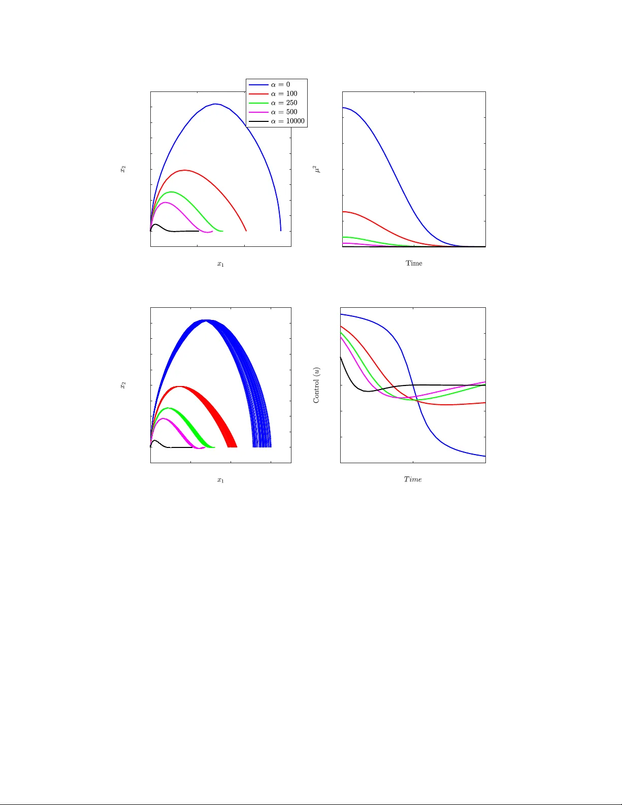
C-DOC: Co-State Desensitized Optimal Con trol V enk ata Ramana Makk apati, Dipank ar Maity , Mehregan Dor, P anagiotis Tsiotras Sc ho ol of Aerospace Engineering Georgia Institute of T echnology A tlanta, GA 30332-0150 { mvramana, dmaity, mehregan.dor, tsiotras } @gatech.edu Octob er 2, 2019 Abstract In this pap er, co-states are used to develop a framework that desensitizes the optimal cost. A general form ulation for an optimal con trol problem with fixed final time is considered. The prop osed scheme in volv es elev ating the parameters of interest in to states, and further augmen ting the co-state equations of the optimal control problem to the dynamical mo del. A running cost that p enalizes the co-states of the targeted parameters is then added to the original cost function. The solution obtained by minimizing the augmen ted cost yields a con trol which reduces the disp ersion of the original cost with resp ect to parametric v ariations. The relationship betw een co-states and the cost-to-go function, for any giv en con trol law, is established substan tiating the approach. Numerical examples and Mon te-Carlo sim ulations that demonstrate the prop osed scheme are discussed. 1 In tro duction Obtaining robust solutions against parametric v ariations in optimal control problems is a requiremen t in v arious applications, particularly in the fields of aerospace and robotics. F or many problems, it is essen tial that for a given p erformance criterion, one can also ensure minimal disp ersion in the total cost, in spite of v ariations in the problem parameters. A simple example w ould be the case of finding a minimum-time tra jectory b etw een tw o p oin ts (cities) on a map when a tra jectory with trav el time that is insensitiv e to traffic flo w v ariations is desirable. In this example, the tra jectory designer is in terested in finding a go o d trade-off b et ween the minim um cost solution and a solution that is less sensitive to v ariations in the mo del parameters (the traffic flo w in the previous example). Solutions obtained b y existing optimal control theory are mo del-dependent, and their resilience to v ariations in uncertain system parameters is not guaranteed. A great deal of researc h has b een performed in robust con trol that primarily fo cuses on the stabilization of systems under uncertain ty and H ∞ optimal control [ 1 , 2 ]. Previous attempts hav e primarily aimed at stabilit y and p erformance criteria defined ov er an infinite horizon [ 3 , 4 ]. Questions regarding the sensitivity of the tra jectory (or the cost) explicitly and its implications on the p erformance ha ve been largely o verlooked. In [ 5 ], the authors hav e addressed the implications of parametric uncertainties ov er a finite horizon using linear matrix inequalities (LMIs), ho wev er, the problem do es not address the sensitivity of the p erformance with respect to the parameters. T raditionally , robust optimal con trol [ 6 – 9 ] and feedbac k con trol syn thesis [ 10 ] ha ve b een used to address the issue of parametric uncertain ty , with an inherent trade-off b et ween cost and robustness to b e decided. Indeed, the increased cost is incurred due to additional control effort, in magnitude or o ver time. The main goal of desensitize d optimal c ontr ol (DOC) is to alleviate the additional effort induced on to the control feedback loop by , instead, picking a tra jectory which is less sensitive to v ariations under parametric uncertain ty . Desensitization of a solution can include addressing the problem of minimizing v ariations: a) in the optimal tra jectory; b) in the final state; or c) in the optimal cost under v ariation in model parameters, for a giv en 1 optimal control problem. The former tw o cases w ere dealt with in our previous w ork [ 11 ]. Three differen t form ulations that employ sensitivit y functions were put forth which desensitize either entire tra jectories or the state at a particular time (e.g., final time). An approach to desensitize the cost for an optimal control problem with fixed final time is presen ted in this pap er. T o this end, we recall that the co-states in an optimal control problem are a measure of the sensitivit y of the v alue function with resp ect to the states along the optimal tra jectory [ 12 , 13 ]. In this pap er, we first prov e that the co-states indeed capture sensitivit y of the c ost-to-go function with respect to p erturbations in the state giv en any prescribed control law u ( t ), not just the optimal one. Using this fact, a new approac h to solve the DOC problem is presen ted. Early work on tra jectory sensitivit y design include those of Winsor and Ro y [ 14 ], who dev elop ed a tec h- nique to design controllers that provide assurance for system p erformance under mathematical mo deling inaccuracy . The feasibilit y of the technique w as established with appropriate sim ulation results. Ho wev er, their work has b een restricted to linear systems. F ollowing that work, sev eral approac hes including sensitivit y- reduction for linear regulators, using increased-order augmen ted system [ 15 ], mo dification of w eighting matrix [ 16 ], feedback [ 17 , 18 ], and an augmented cost function [ 19 , 20 ], were all thoroughly analyzed. The approac h of using an augmented cost function was further tested on the linear quadratic regulator (LQR) problem, whic h was later applied for activ e susp ension con trol in passenger cars [ 20 ]. The w ork by Seywald et al. on desensitized optimal con trol makes use of sensitivity matrices to obtain an optimal open-lo op tra jectory that is insensitive to first-order parametric v ariations [ 21 , 22 ]. The prop osed approac h elev ates the parameters of interest to system states, and defines a sensitivit y matrix that provides the first-order v ariation in the states at time t , given the v ariation in the states at some time t 0 ( t 0 ≤ t ). An appropriate sensitivity cost is added to the existing cost function, and the dynamics of the sensitivit y matrix is augmented in the system dynamics to solve the resulting optimal con trol problem. The approac h was later extended to optimal control problems with control constraints [ 23 ], and it was used to solve the Mars pinp oin t landing problem [ 24 ]. Some extensions to the landing problem include considering uncertainties in atmospheric densit y and aero dynamic characteristics [ 25 ], and using direct collo cation and nonlinear programming [ 26 ]. Ho wev er, the sensitivit y matrix based approaches [ 21 , 22 ] requires propagating the original states, the targeted parameters, and the elemen ts in the sensitivit y matrix, resulting to a total of ( n + ` ) 2 + n + ` n umber of states. An alternative approach w as presen ted in [ 11 ] where the dimensionalit y of the state-space for the augmented problem is reduced to n + n` , using traditional sensitivity functions. Also, techniques based on sensitivit y matrices hav e close connections with co v ariance tra jectory-shaping, whic h was studied b y Zimmer [ 27 ] and Small [ 28 ]. A more detailed discussion on the existing metho ds for desensitized con trol can b e found in [ 29 ]. The contributions of this pap er are summarized as follows: First, we mathematically prov e (Theorem 3.1 ) the fact that for an y giv en con trol law, the co-states of an optimal control problem capture the first- order v ariations of the cost-to-go function given the v ariations in the system states. Second, w e provide an approac h to desensitize (reduce the v ariations of ) the cost with resp ect to parametric v ariations b y elev ating the parameters to system states, and then p enalizing the asso ciated co-states of the optimal con trol problem. Third, it is shown that the co-states and the sensitivity matrices (in Ref. [ 22 ]) are related. The approach is demonstrated on the Zermelo’s na vigation problem, and on a standard linear system thereby establishing its efficacy . The rest of the pap er is organized as follows. Section 2 presen ts some preliminaries and formulates the problem addressed in this w ork. Section 3 first presen ts a deriv ation of the relationship betw een the cost- to-go function and the co-states, and then provides an approach to solv e the co-state based desensitized optimal control (C-DOC) problem. Section 4 demonstrates the proposed approac h with tw o examples. It also contains imp ortan t observ ations which p oin t at some n uances of the approach. Section 5 discusses the relation betw een co-states and sensitivit y matrices. Section 6 concludes the pap er with some directions for future w ork. 2 2 Bac kground and Preliminaries Consider a standard optimal con trol problem of the form inf u J ( u, p ) , φ ( x ( t f ) , t f ) + Z t f t 0 L ( x ( t ) , u ( t ) , t ) d t, (1) sub ject to ˙ x = f ( x, p, u, t ) , x ( t 0 ) = x 0 , , (2a) ψ ( x ( t f ) ,t f ) = 0 , (2b) where t ∈ [ t 0 , t f ] denotes time, with t 0 b eing the initial time and t f b eing the final time (both assumed to b e fixed), p ∈ P ⊂ R ` are ` unkno wn, p ossibly time-v arying, model parameters, x ( t ) ∈ R n denotes the state, with x 0 b eing the fixed state at t 0 . The control u ∈ U = { Piecewise Con tinuous (PW C) , u ( t ) ∈ U, ∀ t ∈ [ t 0 , t f ] } , with U ⊆ R m b eing the set of allo wable v alues of u ( t ), φ : R n × [ t 0 , t f ] → R , the terminal cost function, and L : R n × R m × [ t 0 , t f ] → R , the running cost. Finally , ψ : R n × [ t 0 , t f ] → R k is a function representing k -n umber of constrain t equations at the final time. The ab o ve problem is to be solv ed b y finding the optimal con trol u ∗ ∈ U that minimizes the cost function in ( 1 ). The solution in volv es the optimal tra jectory x ∗ ( t ), t ∈ [ t 0 , t f ], determined from ˙ x ∗ ( t ) = f ( x ∗ ( t ) , p, u ∗ ( t ) , t ) sub ject to x ∗ ( t 0 ) = x 0 , and the optimal cost J ∗ = φ ( x ∗ ( t f ) , t f ) + R t f t 0 L ( x ∗ ( t ) , u ∗ ( t ) , t ) d t . The system dynamics represen ted b y the function f ( x, p, u, t ) con tains the mo del parameters p whic h are assumed to be constant. It is understo od that the optimal solution (constituting the cost, and the tra jectory) is mo del-sensitiv e and, if changes in the parameters p o ccur at any time t ∈ [ t 0 , t f ], then the optimality of the obtained solution is not guaran teed. Consequently , the optimal control problem has to b e resolv ed for eac h new v alue of the parameter vector. If the optimal solution u ∗ is used despite the parameter v ariations, one can exp ect a disp ersion in the optimal tra jectory (and/or cost J ∗ ). With a motiv ation to minimize the disp ersion of the final state x ∗ ( t f ) of the optimal solution, under parametric uncertain ties, Seywald and Kumar constructed an augmented cost function using sensitivit y matrices [ 21 ]. The approach goes as follows. First, the parameters of interest and the corresp onding en tries in the sensitivit y matrix are elev ated to states, and the augmented state [ ˜ x > (v ec S ) > ] > , where ˜ x = [ x p ] > , along with the corresp onding dynamics and initial conditions are deriv ed. The sensitivit y of the vector ˜ x ( t ) 1 at time t with respect to perturbations in the initial state v ector ˜ x ( t 0 ) = ˜ x 0 is denoted as S ( t | t 0 , ˜ x 0 ) That is, S ( t | t 0 , ˜ x 0 ) = ∂ ˜ x ( t | t 0 , ˜ x 0 ) ∂ ˜ x 0 . (3) The dynamics of the state ˜ x can b e written as ˙ ˜ x = ˜ f ( ˜ x, u, t ) = [ f > ( x, p, u, t ) 0 1 × ` ] > , ˜ x ( t 0 ) = ˜ x 0 = [ x > 0 p > 0 ] > , (4) and ˙ S ( t | t 0 , ˜ x 0 ) = ∂ ˜ f ∂ ˜ x S ( t | t 0 , ˜ x 0 ) , S ( t 0 | t 0 , ˜ x 0 ) = I ( n + ` ) , (5) where p 0 is the nominal v alue of the parameter v ector, and where S ( t | t 0 , ˜ x 0 ) represen ts the sensitivity of the v ector ˜ x ( t ) at time t with respect to p erturbations in the initial state v ector ˜ x ( t 0 ). The augmen ted cost function, given in ( 6 ) b elo w, is then minimized to obtain an optimal solution with the final state being “desensitized” with resp ect to the parameter v ariations J s ( u, p ) = J ( u, p ) + Z t f t 0 k vec  S ( t f | t 0 , ˜ x 0 ) S ( t | t 0 , ˜ x 0 ) − 1  k 2 Q ( t )  d t, (6) 1 F rom time to time w e will denote ˜ x ( t ) as ˜ x ( t | t 0 , ˜ x 0 ) to explicitly represent the dep endency on the initial conditions ˜ x 0 = [ x ( t 0 ) > p ( t 0 ) > ] 3 with Q ( t ) ≥ 0 , for all t ≥ t 0 . Note that the sensitivity matrix of Seyw ald in ( 3 ) has the form of a state transition matrix and its prop erties are exploited to construct the sensitivit y of the final state with respect to the v ariations in the state at time t ∈ [0 , t f ], which is then plugged into the running cost ( 6 ). This is elab orated upon in Ref. [ 21 ]. The approac h achiev es the desensitization of the final state. 2.1 Problem F orm ulation In this w ork, we are in terested in desensitizing the cost itself. By denoting J ( u, p ) = Z t t 0 L ( x ( s ) , u ( s ) , s )d t + C ( ˜ x ( t ) , u, t ) , (7) C ( ˜ x ( t ) , u, t ) = Z t f t L ( x ( s ) , u ( s ) , s )d t + φ ( x ( t f ) , t f ) , (8) w e immediately notice that the parametric v ariation at time t , affects the total cost J ( u, p ) only through the cost-to-go C ( ˜ x ( t ) , u, t ). Thus, the sensitivity of the total cost for a parametric v ariation at time t from its nominal v alue p 0 can b e captured through the term S C ( x ( t ) , p 0 , u, t ) = ∂ C ∂ p ( ˜ x ( t ) , u, t )    p = p 0 . (9) There are several wa ys to capture the effect of the parametric v ariations on the cost, one of whic h is to consider the follo wing sensitivity cost J c ( u, p 0 ) = Z t f t 0 k S C ( x ( t ) , p 0 , u, t ) k 2 Q ( t ) d t, (10) for some Q ( t ) ≥ 0, for all t ≥ t 0 . There are three ma jor formulations relev ant to the problem of cost-based desensitization, which are as follo ws. Problem 2.1. Solve inf u ∈U J ( u, p 0 ) (11a) sub ject to J c ( u, p 0 ) ≤ D. (11b) Let us denote the solution of Problem 2.1 to be the “cost-desensitization” function J ( D ) which represents the optimal cost given a b ound on the sensitivity metric. A similar problem is to consider minimizing the sensitivit y of the cost for a given bound on the p erformance index, as presen ted b elo w. Problem 2.2. Solve inf u ∈U J c ( u, p 0 ) (12a) sub ject to J ( u, p 0 ) ≤ J. (12b) Let us denote the solution of Problem 2.2 to b e the “desensitization-cost” function D ( J ). Finding ana- lytical or numerical solutions to J ( D ) or D ( J ) are c hallenging. How ev er, J ( D ) or D ( J ) can b e constructed b y solving the following family optimization problems for all α ∈ [0 , ∞ ). Problem 2.3. Solve inf u ∈U J ( u, p 0 ) + α J c ( u, p 0 ) (13) 4 By observing that the scalar α can b e absorb ed in to the matrix Q ( t ), we will rewrite the ob jetive function in Problem 2.3 as J s ( u ) = J ( u, p 0 ) + J c ( u, p 0 ) . When the sensitivit y cost has zero w eight ( Q ( t ) ≡ 0), we solve problem ( 1 ) and retrieve lim sup D →∞ J ( D ), and as w e increase the weigh t on the sensitivity cost (through Q ( t )), w e arriv e at an optimal con trol whose p erformance is more insensitive to the v ariations in the parameters. In the limit when Q ( t ) → ∞ for all t , w e retriev e lim sup J →∞ D ( J ). In this work, w e will fo cus on minimizing J s ( u ). Detailed analysis of J ( D ) and D ( J ) will app ear elsewhere. The new optimization problem w e are interested in solving is inf u J s ( u ) (14a) sub ject to ˙ x = f ( x, p 0 , u, t ) , x ( t 0 ) = x 0 , (14b) ψ ( x ( t f ) , t f ) = 0 . (14c) The follo wing section presents a formal pro of for the fact that the co-states capture the sensitivit y of the cost-to-go function for an y giv en con trol input ¯ u ( t ), that satisfies the terminal constrain t ( 14c ) with nominal v alue of the parameter p 0 . The result would allow us to p enalize a w eighted norm of the co-states, with their dynamics obtained from the adjoint equations, that desensitizes the cost function with resp ect to the v ariations in the targeted parameters. 3 Co-states and Desensitized Optimal Con trol In this section we characterize the cost-sensitivit y S C ( x ( t ) , p 0 , u, t ) in terms of the co-state pro cess asso ciated with the optimal control problem given b y ( 1 )-( 2b ). The follo wing theorem sho ws that the sensitivit y of the cost-to-go function with respect to the state at time t can b e represen ted by a co-state process λ with certain b oundary conditions at the final time t f . Theorem 3.1. Consider the dynamic al system ˙ x = f ( x, u, t ) , evolving under a given c ontr ol law ¯ u ∈ ¯ U ⊆ U , wher e ¯ U = n ¯ u : [ t 0 , t f ] → R m is PWC , ¯ u ( t ) ∈ U, such that ψ ( x ( t f ) , t f ) = 0 , x ( t f ) = x 0 + Z t f t 0 f ( x ( t ) , ¯ u ( t ) , t ) d t o . Then, for a c ost-to-go function (asso ciate d with the c ost functional ( 1 ) ) with x = x ( t ) C ( x, ¯ u, t ) = φ ( x ( t f ) , t f ) + Z t f t L ( x ( τ ) , ¯ u ( τ ) , τ ) d τ , (15) under the c ontr ol ¯ u ∈ ¯ U , the sensitivity of the c ost-to-go function with r esp e ct to the state x at time t is, λ > ( t ) = ∂ C ∂ x ( x ( t ) , ¯ u, t ) , (16) which ob eys the dynamics ˙ λ > ( t ) = − ∂ H ∂ x ( x ( t ) , ¯ u, λ ( t ) , t ) , (17) wher e H ( x, u, λ, t ) = L ( x, u, t ) + λ > f ( x, u, t ) . (18) F urthermor e, the terminal c ondition for ( 17 ) is given by λ ( t f ) = ∂ φ ∂ x ( x ( t f ) , t f ) . (19) 5 Pr o of. The proof is presented in Appendix 6.1 . It is in teresting to note that the theorem holds not only for the optimal control (a result that follo ws directly from the maximum principle [ 30 ]), but for an y control la w that is piecewise-con tinuous and ensures that the terminal constrain t is met. The C-DOC problem can now b e fully form ulated using this result. F or the C-DOC problem the augmented state is ˜ x = [ x > , p > ] with dynamics given in ( 4 ). The Hamiltonian, defined in Theorem 3.1 , for this system, can be written as H ( ˜ x, u, λ, µ, t ) = L ( x, u, t ) + λ > ˙ x + µ > ˙ p = L ( x, u, t ) + λ > f ( x, p, u, t ) , (20) where λ and µ are the co-states corresp onding to state x and v ector of parameters defined b y p , resp ectiv ely . The corresp onding adjoin t equations are given b y ˙ λ > = − ∂ H ∂ x ( ˜ x, u, λ, µ, t ) = − λ > ∂ f ∂ x ( x, p, u, t ) − ∂ L ∂ x ( x, u, t ) , (21) ˙ µ > = − ∂ H ∂ p ( ˜ x, u, λ, µ, t ) = − λ > ∂ f ∂ p ( x, p, u, t ) . (22) Since the co-states represent the sensitivity of the cost-to-go function for a given con trol input u ( t ) (Theorem 3.1 ), they can be expressed as λ ( t ) > = ∂ C ∂ x ( ˜ x ( t ) , u, t ) , (23) µ ( t ) > = ∂ C ∂ p ( ˜ x ( t ) , u, t ) , (24) for a giv en control u ∈ ¯ U , this results in the tra jectory x ( t ) for t 0 ≤ t ≤ t f , where C ( ˜ x, u, t ) = φ ( x ( t f ) , t f ) + Z t f t L ( x ( τ ) , u ( τ ) , τ ) d τ . Note that p is an augmented state in the giv en problem and affects the cost J through the state x , whose dynamics is a function of p . Since w e ha ve used ˙ p = 0 and p ( t 0 ) = p 0 , w e ha ve ensured that p ( t ) = p 0 . Thus, b y comparing equations ( 9 ) and ( 24 ), we obtain µ ( t ) = S C ( x ( t ) , p 0 , u, t ). Therefore, w eighting the co-state in the existing cost function will ensure that the solution of the augmented problem minimizes the sensitivit y of the cost J with resp ect to parametric v ariations. This results in an updated optimal con trol problem with an augmen ted cost, accounting for the sensitivit y comp onen t, giv en by J s ( u ) = φ ( x ( t f ) , t f ) + Z t f t 0  L ( x ( t ) , u ( t ) , t ) + µ > ( t ) Q ( t ) µ ( t )  d t. (25) Minimizing the cost ( 25 ) sub ject to the dynamics ( 4 ), terminal constraint ( 2b ), and the transversalit y con- ditions ( 19 ) with µ ( t f ) = 0 , (26) yields a desensitized optimal con trol problem for the original problem. Here, Q ( t ) ∈ R ` × ` is a user-defined p ositiv e semi-definite w eighting function and is generally of the form Q ( t ) ≡ diag( α 1 ( t ) , . . . , α ` ( t )) . (27) This co-state based approac h requires formulating 2( n + ` ) n umber of states, as compared to the higher 2( n + ` ) 2 + n + ` states in [ 21 ], employing sensitivity matrices for an optimal control problem. The resulting problem ( 25 ) is t ypically solved b y the off-the-shelf existing solv ers. 6 4 Numerical Examples In many applications, the resulting tra jectories should be insensitiv e with respect to p erturbations and/or uncertain ties within the mo del parameters at sp ecified times along the tra jectory . The following section presen ts some n umerical examples that will aid in understanding the implementation of this tec hnique and will elucidate its subtleties. The sim ulations are obtained using GPOPS-I I [ 31 ]. 4.1 Zermelo’s Na vigation Problem Consider a typical Zermelo’s problem [ 21 ] with currents parallel to the shore ( x 1 ) as a function of x 2 suc h that v current = px 2 , (28) where p is a parameter, whic h is uncertain, and its nominal v alue is p 0 = 10. The problem has to b e desensitized with resp ect to this parameter. The dynamics can b e written as ˙ x 1 = cos( u ) + px 2 , (29) ˙ x 2 = sin( u ) , (30) sub ject to the conditions x 1 (0) = 0 , x 2 (0) = 0 , x 2 ( t f ) = 0 , t f = 1 . F or the case where the state x 1 ( t f ) has to b e maximized, the cost function can b e expressed in the May er form as min u J ( u ) = − x 1 ( t f ) , (31) where u ∈ U =  C 0 , u ( t ) ∈ [0 , 2 π ) , ∀ t ∈ [0 , 1]  and is the control input. Here, optimization of the tra jectory is done with respect to parameter p , which is not precisely known. In order to facilitate desensitization of the cost (in this case the final state x 1 ( t f )) with resp ect to v ariations in the parameter p we first consider the augmen ted dynamics ˙ ˜ x =   ˙ x 1 ˙ x 2 ˙ p   =   cos( u ) + px 2 sin( u ) 0   , (32) with b oundary conditions ˜ x (0) =   x 1 (0) x 2 (0) p (0)   =   0 0 p 0   , x 2 ( t f ) = 0 . (33) The Hamiltonian is giv en by H ( ˜ x, u, λ, µ ) = λ 1 (cos( u ) + px 2 ) + λ 2 sin( u ) , (34) and the adjoin t equations are: ˙ λ 1 = − ∂ H ∂ x 1 = 0 , (35) ˙ λ 2 = − ∂ H ∂ x 2 = − λ 1 p, (36) ˙ µ = − ∂ H ∂ p = − λ 1 x 2 . (37) 7 0 1 2 3 -0.05 0 0.05 0.1 0.15 0.2 0.25 0.3 0.35 0.4 (a) Optimal tra jectories 0 0.5 1 0 0.01 0.02 0.03 0.04 0.05 0.06 (b) µ 2 ( t ) - a measure of sensitivit y 0 1 2 3 -0.05 0 0.05 0.1 0.15 0.2 0.25 0.3 0.35 0.4 (c) Mon te-Carlo simulations 0 0.5 1 -1.5 -1 -0.5 0 0.5 1 1.5 (d) Optimal Con trol ( u ∗ ) Figure 1: Results obtained for the Zermelo’s path optimization problem with differen t lev els of desensitization The cost for the desensitized optimal con trol problem is min u J s ( u ) = − x 1 ( t f ) + Z t f 0 αµ 2 ( t ) d t. (38) The weigh t parameter α is chosen betw een 0 and 10,000. Figure 1 (a) shows the optimal paths obtained for the five different v alues of α in the selected range. As the v alue of α increases, the optimal solution mo ves closer to the shore, minimizing the effect of uncertaint y in the current, which has an effect prop ortional to the distance x 2 . F or α → ∞ , the optimal path would b e mo ving along the shore, i.e., along the x 1 axis. The results obtained from the Monte-Carlo simulations are sho wn in Figure 1 (c) which confirm the exp ected desensitization of the cost x 1 ( t f ), further substantiating the claims. F or the Monte-Carlo simulations, a time-constan t parametric v ariation is enforced, and 100 different v alues betw een [0 . 9 p 0 , 1 . 1 p 0 ] are randomly c hosen to b e p . The trends of the in tegrand in the running cost µ 2 ( t ) (Figure 1 (b)), show that its v alue is steadily decreasing and is almost zero for α = 10 , 000. 8 4.2 Linear Systems Consider an optimal con trol problem of minimizing a quadratic cost J ( u ) = Z t f 0 1 2 ( x > R 1 x + u > R 2 u ) d t, (39) giv en the n -dimensional linear dynamics with parameter vector p ˙ x = A ( p ) x + B ( p ) u, (40) ˙ p = 0 , (41) with initial conditions x (0) = x 0 , p (0) = p 0 , (42) where x ∈ R n , u ∈ R m , p ∈ R ` , A : R ` → R n × n , B : R ` → R n × m , R 1 ≥ 0, R 2 > 0, and t f is fixed. The goal is to desensitize the cost with resp ect to the parameter p . F ollowing the steps to construct the cost term for desensitization, the Hamiltonian is giv en by H = 1 2 ( x > R 1 x + u > R 2 u ) + λ > ˙ x + µ > ˙ p, = 1 2 ( x > R 1 x + u > R 2 u ) + λ > ( A ( p ) x + B ( p ) u ) . (43) The adjoin t equations are ˙ λ > = − ∂ H ∂ x = − x > R 1 − λ > A ( p ) , (44) ˙ µ > = − ∂ H ∂ p = − ( x > ⊗ λ > ) ∂ ∂ p v ec( A ( p )) − ( u > ⊗ λ > ) ∂ ∂ p v ec( B ( p )) . (45) where λ and µ are the co-states of x and p , resp ectiv ely . Since the cost has to b e desensitized with resp ect to p , the augmen ted cost that has to b e minimized for the C-DOC problem is giv en by J s ( u ) = Z t f 0 1 2 ( x > R 1 x + u > R 2 u + µ > Qµ ) d t. (46) T o demonstrate the results, we consider a one-dimensional linear system with the dynamics ˙ x = ax + bu with initial condition x (0) = 1, and let R 1 = R 2 = 2, t f = 20. W e first analyze the case where b is the uncertain parameter with its nominal v alue as b 0 = 1, and a = − 1. The solutions obtained for Q = 0 and 1 , 000 are sho wn in Figure 2 . Note that the sensitivit y measure ( µ 2 ( t )) in Figure 2 (b) is low er for the desensitized solution. Since b is the source of uncertaint y that p erturbs the tra jectory (and even tually the cost), b y in tro ducing desensitization ( Q = 1 , 000), it can be observ ed from Figure 2 (d) that the control go es to zero earlier compared to the non-desensitized solution. By making the con trol zero, the source of uncertaint y is remo v ed from the system. The results obtained from the Mon te-Carlo sim ulations with b ∈ [0 . 8 b 0 , 1 . 2 b 0 ] are sho wn in Figure 2 (c), whic h suggests that the v ariation in the cost for the desensitized solution is significan tly lo wer. The res ults for the case where a is the uncertain parameter with its nominal v alue as a 0 = − 1 (stable), and b = 1 are shown in Figure 3 . Since a is the source of uncertaint y , b y switching on the desensitization ( Q = 1 , 000), it can b e observed from Figure 3 (a) that the state approac hes zero faster compared to the non- desensitized solution. Consequen tly , from the Monte-Carlo sim ulations ( a ∈ [0 . 8 a 0 , 1 . 2 a 0 ]), it can b e observed that the v ariations in the optimal tra jectory (Figure 3 (c)), and the cost (Figure 3 (d)) are significan tly low er for the desensitized solution, though the cost for the same is higher whic h is a trade-off. The error bars in Figure 3 (d) represen t the minimum and the maxim um costs obtained form the Monte-Carlo results where the corresp onding grey bars represent the nominal costs with a = a 0 . 9 0 5 10 15 20 -0.2 0 0.2 0.4 0.6 0.8 1 (a) Optimal tra jectories 0 5 10 15 20 0 0.005 0.01 0.015 (b) µ 2 ( t ) - a measure of sensitivit y 0 5 10 15 20 -0.2 0 0.2 0.4 0.6 0.8 1 (c) Mon te-Carlo simulations 0 5 10 15 20 -0.5 -0.4 -0.3 -0.2 -0.1 0 0.1 (d) Optimal Con trol ( u ∗ ) Figure 2: Results obtained for an LQR problem with B matrix being uncertain W e also consider an unstable system with a ∈ [0 . 8 a 0 , 1 . 2 a 0 ] being the uncertain parameter with a 0 = 0 . 1. Figure 4 (a) shows the Mon te-Carlo results, and the b eha vior is similar to the one in the previous example except that the tra jectories are no w divergen t b ecause the system matrix is unstable. A more interesting case is a marginally stable system with a 0 = 0, and a ∈ [ − 0 . 2 , 0 . 2]. The corresp onding results can b e found in Figure 5 . In the previous cases, although a parametric v ariation in a is studied, suc h v ariations did not change the stabilit y of the system, i.e., if the nominal system is stable, then the system with parametric v ariation is stable as well. Since a can be b oth stable and unstable, the optimal con trol obtained for the nominal system without desensitization will be less effective com bating the instabilities compared to the desensitized solution, as can be seen from the disp ersion in tra jectories (and costs) in Figure 5 . 10 0 5 10 15 20 -0.2 0 0.2 0.4 0.6 0.8 1 (a) Optimal tra jectories 0 5 10 15 20 -1.4 -1.2 -1 -0.8 -0.6 -0.4 -0.2 0 0.2 (b) Optimal Con trol ( u ∗ ) 0 5 10 15 20 -0.2 0 0.2 0.4 0.6 0.8 1 (c) Mon te-Carlo simulations 0 0.2 0.4 0.6 0.8 1 (d) Cost ( J ) Figure 3: Results obtained for an LQR problem with a stable A matrix being uncertain 5 Discussion: Relation b et w een the Sensitivit y Matrix and co- states In this section w e address the relationship b et w een the sensitivity matrix defined in ( 3 ) and the co-states λ . Let us note that, λ > ( t ) = ∂ C ∂ x ( x ( t ) , u, t ) , (47) 11 0 5 10 15 20 -0.2 0 0.2 0.4 0.6 0.8 1 (a) Mon te-Carlo simulations 0 0.5 1 1.5 (b) Cost ( J ) Figure 4: Results obtained for an LQR problem with an unstable A matrix b eing uncertain (red: Q = 0, green: Q = 1 , 000). 0 5 10 15 20 -1 0 1 2 3 4 5 6 7 (a) Mon te-Carlo simulations 0 20 40 60 80 100 120 140 160 180 (b) Cost ( J ) Figure 5: Results obtained for the LQR problem with a = 0 (red: Q = 0, green: Q = 1 , 000). whic h can b e expressed as λ > ( t ) = ∂ C ( x ( t ) , u, t ) ∂ x 0  ∂ x ( t ) ∂ x 0  − 1 = ∂ C ( x ( t ) , u, t ) ∂ x 0 S ( t | t 0 , x 0 ) − 1 , (48) where S ( t | t 0 , x 0 ) = ∂ x ( t ) ∂ x 0 is the sensitivit y of the state at time t along the tra jectory with respect to v ariation in its initial condition x 0 [ 21 ]. Note that the dep endency of x ( t ), t ≥ t 0 on t 0 and x 0 (initial conditions) 12 is implicit. The relationship b etw een the co-state and the sensitivity matrix in ( 48 ) can b e generalized to obtain the sensitivit y of the solution with regards to the state at an y other time t 0 as λ > ( t ) = ∂ C ( x ( t ) , u, t ) ∂ x ( t 0 ) ∂ x ( t 0 ) ∂ x ( t ) , (49) = ∂ C ( x ( t ) , u, t ) ∂ x ( t 0 ) S ( t | t 0 , x ( t 0 )) − 1 ∀ t, t 0 ∈ [ t 0 , t f ] . (50) Therefore, λ ( t ) = S ( t | t 0 , x ( t 0 )) −>  ∂ C ( x ( t ) , u, t ) ∂ x ( t 0 )  > , (51)  ∂ C ( x ( t ) , u, t ) ∂ x ( t 0 )  > = S ( t | t 0 , x ( t 0 )) > λ ( t ) . (52) F rom the ab o ve expressions, we observ e that the sensitivity matrix S ( t | t 0 , x ( t 0 )) > is essentially the tran- sition matrix b et w een the co-states λ ( t ) and the partial of the cost-to-go function at time t with resp ect to the state at time t 0 , i.e., the sensitivity of the cost-to-go function at time t with respect to the state at time t 0 < t . 6 Conclusion W e attempt to exploit the co-states to obtain tra jectories that are less sensitive to parametric v ariations. It is established that the co- states, defined by the Hamiltonian and the adjoin t equations, capture the sensitivit y of a cost-to-go function for any arbitrary con trol la w. This has led to the idea of inserting the co-states into the cost function and then studying its implications in the context of DOC. In particular, this approach has b een used to solve the problem of cost desensitization with respect to v ariation in system parameters. The results suggest that v ariations to parametric uncertaint y and optimalit y can be balanced using this approach through the c hoice of an appropriate weigh ting parameter. The n umerical sim ulations give promising results that v alidate the theory . The proposed approac h can b e used to look at some other in teresting problems, esp ecially related to robust optimal con trol. It is also of in terest to closely study its connections with co v ariance-steering for sto c hastic dynamical systems [ 32 ]. Ac kno wledgmen t This w ork has b een supported by NSF a ward CMMI-1662542. App endix 6.1 Pro of of Theorem 3.1 F or a fix control ¯ u , the cost-to-go from any state x at time t is C ( x, ¯ u, t ) = φ ( x ( t f ) , t f ) + Z t f t L ( x ( s ) , ¯ u ( s ) , s )d s where x ( t ) = x . 13 Let the p erturb ed state at time t be represented by x ( t, α ) = x ( t ) + αδx ( t ) where α ∈ [0 , α 0 ) for some α 0 > 0, and δ x ( t ) ∈ R n . With this perturbation the new cost-to-go is C ( x + αδ x, ¯ u, t ) = φ ( x ( t f , α ) , t f )+ Z t f t L ( x ( s, α ) , ¯ u ( s ) , s )d s where x ( s, α ) denotes the p erturbed state at time s ≥ t . By denoting x ( s, α ) = x ( s, 0) + αδ x ( s ) , for all s ≥ t , we obtain δ ˙ x ( s ) = f x ( x ( s, 0) , ¯ u ( s ) , s ) δ x ( s ) + O ( α ) , where O ( α ) is such that lim α → 0 O ( α ) = 0. Consequen tly , δ x ( s ) = Γ( s, t ) δ x ( t ) + O ( α ) where Γ( s, t ) is the state transition matrix corresponding to the matrix f x ( x ( s, 0) , u ( s ) , s ). Therefore, C ( x + α δx, ¯ u, t ) − C ( x, ¯ u, t ) = αφ x ( x ( t f , 0) , t f )Γ( t f , t ) δ x + α  Z t f t L x ( x ( s, 0) , u ( s ) , s )Γ( s, t )d s  δ x + O ( α 2 ) and th us, lim α → 0 + C ( x + αδ x, ¯ u, t ) − C ( x, ¯ u, t ) α = h φ x ( x ( t f , 0) , t f )Γ( t f , t ) + Z t f t L x ( x ( s, 0) , u ( s ) , s )Γ( s, t )d s i δ x, = ⇒ C x ( x, ¯ u, t ) = φ x ( x ( t f , 0) , t f )Γ( t f , t ) + Z t f t L x ( x ( s, 0) , ¯ u ( s ) , s )Γ( s, t )d s. A t this p oin t, if we denote λ > , C x ( x, ¯ u, t ) . W e then hav e ˙ λ > = − λ > f x − L x , since ˙ Γ( s, t ) = − Γ( s, t ) f x ( x ( t, 0) , u ( t ) , t ). F urthermore, λ ( s ) satisfies the terminal condition λ ( t f ) = φ x ( x ( t f ) , t f ). Th us, if we define the Hamiltonian as H = L + λ T f , it follo ws that ˙ λ > = − ∂ H ∂ x and this λ represen ts the first order v ariation in cost-to-go with boundary condition λ ( t f ) = φ x ( x ( t f ) , t f ) . The result follo ws. References [1] Shank ar P Bhattacharyy a and Lee H Keel. Robust con trol: the parametric approac h. In A dvanc es in Contr ol Educ ation , pages 49–52. Elsevier, 1995. [2] Kemin Zhou and John Comstock Doyle. Essentials of R obust Contr ol , volume 104. Pren tice hall Upper Saddle Riv er, NJ, 1998. 14 [3] Ian P etersen and Rob erto T emp o. Robust control of uncertain systems: Classical results and recent dev elopments. Automatic a , 50(5):1315–1335, 2014. [4] Y ouyi W ang, Lihua Xie, and Carlos E De Souza. Robust control of a class of uncertain nonlinear systems. Systems & Contr ol L etters , 19(2):139–149, 1992. [5] F rancesco Amato, Marco Ariola, and P eter Dorato. Finite-time con trol of linear systems sub ject to parametric uncertain ties and disturbances. Automatic a , 37(9):1459–1463, 2001. [6] Kemin Zhou, John Doyle, and Keith Glov er. R obust and Optimal Contr ol , v olume 40. Prentice hall New Jersey , 1996. [7] Stefan K¨ ork el, Ek aterina Kostina, Hans Georg Bock, and Johannes P . Sc hl¨ oder. Numerical metho ds for optimal control problems in design of robust optimal exp erimen ts for nonlinear dynamic pro cesses. Optimization Metho ds and Softwar e , 19(3-4):327–338, 2004. [8] Zoltan K. Nagy and Richard D. Braatz. Op en-loop and closed-lo op robust optimal control of batch pro cesses using distributional and worst-case analysis. Journal of Pr o c ess Contr ol , 14(4):411 – 422, 2004. [9] F eng Lin and R. D. Brandt. An optimal control approac h to robust control of robot manipulators. IEEE T r ansactions on R ob otics and Automation , 14(1):69–77, F eb 1998. [10] Isaac M. Horowitz. Synthesis of F e e db ack Systems . Academic Press, 1963. [11] V. R. Makk apati, M. Dor, and P . Tsiotras. T ra jectory desensitization in optimal control problems. In IEEE Confer enc e on De cision and Contr ol (CDC) , pages 2478–2483, Dec 2018. [12] Arth ur E Bryson and Y u-Chi Ho. Applie d Optimal Contr ol , c hapter 4.2, pages 134–135. Hemisphere Publishing, 1975. [13] D. W. Peterson. On sensitivit y in optimal con trol problems. Journal of Optimization The ory and Applic ations , 13(1):56–73, 1974. [14] C. Winsor and R. Roy . The application of sp ecific optimal con trol to the design of desensitized mo del follo wing control systems. IEEE T r ansactions on A utomatic Contr ol , 15(3):326–333, 1970. [15] R. Subba yyan, V. V. S. Sarma, and M. C. V aithilingam. An approac h for sensitivity-reduced design of linear regulators. International Journal of Systems Scienc e , 9(1):65–74, 1978. [16] C. V erde and P . M. F rank. Sensitivit y reduction of the linear quadratic regulator b y matrix modification. International Journal of Contr ol , 48(1):211–223, 1988. [17] G. Zames. F eedbac k and optimal sensitivit y: Mo del reference transformations, m ultiplicative seminorms, and appro ximate inv erses. IEEE T r ansactions on Automatic Contr ol , 26(2):301–320, April 1981. [18] Bor-Chin Chang and J. P earson. Optimal disturbance reduction in linear m ultiv ariable syste ms. IEEE T r ansactions on A utomatic Contr ol , 29(10):880–887, Oct 1984. [19] D. L. T ang. The design of a desensitized con troller - a sensitivity function approach. In Pr o c e e dings of the Americ an Contr ol Confer enc e , pages 3103–3111, May 1990. [20] F ederico Cheli, F erruccio Resta, and Edoardo Sabbioni. Observer design for activ e susp ension control for passenger cars. In Pr o c e e dings of the ASME Confer enc e on Engine ering System Design and A nalysis , pages 1–9, T orino, Italy , 2006. [21] Hans Seyw ald and Renjith R Kumar. Desensitized optimal tra jectories. A dvanc es in the Astr onautic al Scienc es , 93:103–115, 1996. 15 [22] Kevin Seyw ald and Hans Seyw ald. Desensitized optimal con trol. In AIAA SciT e ch F orum , San Diego, CA, Jan uary 2019. AIAA Paper 2019-0651. [23] Hans Seyw ald. Desensitized optimal tra jectories with control constraints. A dvanc es in the Astr onautic al Scienc es , 114:737–743, 2003. [24] Haijun Shen, Hans Seywald, and Ric hard W Po well. Desensitizing the minimum-fuel p o wered descen t for Mars pinpoint landing. Journal of Guidanc e, Contr ol, and Dynamics , 33(1):108–115, 2010. [25] H. Xu and H. Cui. Robust tra jectory design sc heme under uncertainties and perturbations for Mars en try v ehicle. In IEEE International Confer enc e on Computational Intel ligenc e Communic ation T e chnolo gy , pages 762–766, 2015. [26] Sh uang Li and Y uming Peng. Mars en try tra jectory optimization using DOC and DCNLP. A dvanc es in Sp ac e R ese ar ch , 47(3):440–452, 2011. [27] Scott Jason Zimmer. R e ducing sp ac e cr aft state unc ertainty thr ough indir e ct tr aje ctory optimization . PhD thesis, The Univ ersity of T exas at Austin, 2005. [28] T odd Vincent Small. Optimal tra jectory-shaping with sensitivity and cov ariance tec hniques. Master’s thesis, Massac husetts Institute of T ec hnology , 2010. [29] Alexander W einmann. Unc ertain Mo dels and R obust Contr ol . Springer Science & Business Media, 2012. Chapter 10. [30] Lev Semeno vich P ontry agin. Mathematic al The ory of Optimal Pr o c esses . Routledge, 2018. [31] Mic hael A. P atterson and Anil V. Rao. GPOPS-II: A MA TLAB soft ware for solving m ultiple-phase opti- mal con trol problems using hp-adaptiv e Gaussian quadrature c ollocation methods and sparse nonlinear programming. A CM T r ans. Mathematic al Softwar e , 41(1):1:1–1:37, Octob er 2014. [32] K. Ok amoto, M. Goldsh tein, and P . Tsiotras. Optimal cov ariance con trol for sto c hastic systems under c hance constraints. IEEE Contr ol Systems L etters , 2(2):266–271, 2018. 16