An Improved Quantum Projection Filter

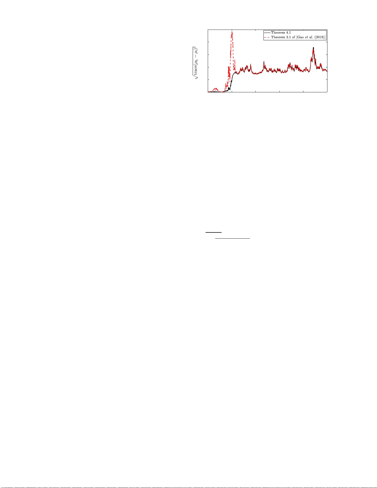
An Improv ed Quantum Projection Filter Qing Gao ∗ Guofeng Zhang † Ian R. Petersen ‡ October 1, 2019 Abstract This work extends the previous quantum projection filtering scheme in [Gao Q., Zh ang G., & Petersen I. R. (20 19). An exponential quan tum projec tion filter f or o p en q uantum sys- tems. Automatica , 99, 5 9-68.] , by a dding a n optimality ana l- ysis result. A reform u lation o f the quan tu m projection filter is derived by min imizing the truncated Stratonovich stochastic T aylor expansion o f the d ifference be twe e n the tr ue qu a ntum trajectory and its appr o ximation on a lower-dimensional sub- manifold through q uantum information g e ometric tech n iques. Simulation r e sults f or a q u bit examp le dem onstrate be tter ap- proxim a tion perf ormance for the ne w quan tu m p rojection fil- ter . Keywords. Quantum filters; quantum projectio n filters; Stratonovich stoc hastic T aylor expansions; quantum info rma- tion g eometry . 1 Introd uction The quantum filter in th e Schr ¨ odinger pictur e, also k nown as the quan tum stochastic master equation , is a stochas- tic differential equation (SDE) that g overns the time ev olu tio n of the state of a co n tinuously m o nitored quan- tum system ([Belavkin (199 2)], [Bouten et al. ( 2007)], [Gardiner & Zoller (2000)]). In the implemen tatio n of many quantum tec h nologie s such as measur e ment-based quantum feedback con trol [W iseman & Milburn (201 0)], onlin e calcu- lation of the quantum filter equation is an essential requirement which is, however , often comp utationally deman ding when the quantum system und er consideration has a hig h dimension ality ∗ School of Automation Scienc e and E lectri cal Engineering, Beihang Uni- versi ty , Be ijing 10 0191, Chi na. (qing.gao.cha nce@gmai l.com) † Departmen t of Applied Mathemati cs, Hong Kong Polytec h- nic Univ ersity , Hong Kon g, China (guofeng.zha ng@polyu.ed u.hk, https://www.po lyu.edu.hk/ama/p rofile/gfzhang/ ). ‡ Researc h School of Electrical , Energy and Mate rials Engine ering, The Aust ralian Nat ional Uni versity , Canberra A CT 2601, Australia . (i.r .petersen@gma il.com). ([Gao et al. (2 016)], [Song et al. (2016)]). For example, to derive the ato mic excitation probability for a two-level ato m driven by counter-propag ating pho tons via its quantu m filter, a total of 63 scalar valued SDEs has to b e numerically solved [Dong et al. (2019)]. In general, obtainin g the solution to the quantum filter equatio n for an n − d imensional quantum system in volves solving a system of n 2 − 1 scalar valued SDEs. It is thus particularly u sef ul to de velop a c o mputation ally m ore efficient appro x imation mod e l for the quan tum filter equ a tion to speed up the estimatio n of the c onditiona l quantum state. In th e past decades, research on appro ximation of the q uantum filter equ ation has b e en pop u lar , for exam- ple, see ([ E mzir et al. (20 17)], [Rouch on & Ralph (2 015)], [Tsang (2 014)]). Among the existing results, one inter- esting appro x imation scheme is the quantum projection fil- tering approa c h , whic h is mo tiv ated by the p ioneerin g work by Brig o, Hanzon and LeGland ([Brig o et al. (19 98)], [Brigo et al. (1 999)]) where classical (non-q u antum) stoch as- tic dyn amic systems were considered . The first re- sult o n quantum p rojection filterin g can be fou nd in [van Handel & Mabuchi (200 5 )] which , h owe ver, requires ex- act prior knowledge of an in variant set for the solutions to the quantum filter equatio n and has limited applicatio ns in m ore complex cases. A less restrictive approach was pr oposed in [Nielsen et al. ( 2009)] where a two-le vel quantu m system was considered . In our r ecent work [Gao e t al. (2019 ) ] , we proposed an ex- ponen tial quantum projectio n filtering appro ach t hat is applica- ble to general open quan tum systems. The ba sic idea can be summarized as follows. First, a lower dimensiona l differential submanifo ld emb e dded in the quantum system state space is chosen and endowed with a metric structure. Then, an orthogo- nal projection operation is defined in terms of this metric and is used to project the coef ficien ts of the quantum filter equatio n in Stratonovich f orm to the tang ent vector space of the submani- fold. In this way , a new curve is generated on the subman ifold, which serves as an app roximatio n to the o riginal q uantum tra- 1 jectory . It can be inferred from elemen tar y lin ear algebr a that the coef ficients of this ne w curve are optimal app roximatio ns to the coefficients of the quantum filter equatio n . Nev ertheless, it is still questionable h ow goo d an appro ximation the new cur ve is fo r the o riginal quantum trajecto r y . In this pap er , we p resent an alterna ti ve design o f quantum projection filters using Straton ovich stochastic T ay lor expan- sions [Kloed e n & Platen (199 9)] and quantu m infor mation ge- ometric techn iques [Amar i & Nagaoka (200 0) ], motiv ate d by the r e search work in [A r mstrong & Brigo (2 019)] whe r e clas- sical stoch astic dyn amic systems were considered. This de- sign is o ptimal in the sense that the truncated Stratonovich stochastic T aylor expa n sion of the difference between the o rig- inal quantu m tr ajectory and its approx imation on a lower - dimensiona l submanif old is minimiz e d in the mean square sense. An interestin g c onclusion is that for a special class of open quan tum systems, th e propo sed m ethod and th e one in [Gao et al. (2 019)] yield th e same op timal quan tum p r ojection filter equatio n (see Corollar y 4.1). W e use simulation results from a fo ur-le vel quan tum system example to demonstrate th e improved a pprox im ation capability o f th e pr oposed app roach over the one in [ Gao et al. (20 19)], in the gen eral cases. Notatio n. The Rom an type character i is used to distin- guish th e imaginary unit i= √ − 1 from the index i . For any two n − dimension a l squar e matr ices A and B , A ⊗ B means the tensor prod uct of A and B and [ A, B ] = AB − B A rep re- sents the commutator of A and B . A † represents the complex conjuga te transpose of A , T r( A ) is the tr ace of matrix A , and k A k F = p T r( A † A ) is the Hilbert- Schmidt norm of ma tr ix A . I p is the p − d imensional id entity matrix for an integer p . R n represents the n -dimen sional real vector spac e . 2 The Quantum Filter and The Quan- tum Pr ojection Filter The qu antum system model used in this paper follows the one in [Bouten et a l. (200 7) ]. W e consider a finite-dimen sional quantum system Q that has a Hilbert space H Q with dim H Q = n < ∞ , an d we use a sy mmetric Fock space E to mod e l the quantum bath . The quantum system Q interacts with the quan- tum bath on which c ontinuo u s obser vations are made throug h a homod yne detector . The co mposite system is initially pre p ared in the state ρ total = ρ 0 ⊗ ρ vacuum , where ρ 0 is some state on H Q and ρ vacuum is the vacuum state on E . By using quantum filterin g theory , the dyn amics of the quan- tum den sity oper ator of Q con d itioned on th e past h istory of the observation pr ocess satisfy the f ollowing I t ˆ o quantum SDE ([Belavkin (1992 )], [Bouten et al. (2 007)]): dρ t = L † L,H ( ρ t ) dt + ( Lρ t + ρ t L † − ρ t T r( ρ t ( L + L † ))) ×  d Y t − T r( ρ t ( L + L † ) dt  , (1) where H is the quan tu m system Hamilton ian, L is the coupling strength o perator, L † L,H is th e adjo int of the Lind b lad generato r L L,H ( X ) = − i [ H , X ] + LX L † − 1 2 ( L † LX + X L † L ) , and Y t is the W iener type classical photocur r ent sign al g enerated by the ho modyn e detector . The nonlin ear SDE (1) is known as the q uantum filter or the quantum stochastic master equation . In the rest o f th is paper, howe ver , we will work on the fo llowing equiv ale n t Stratonovich typ e unn ormalized lin ear form of (1) fo r the sake of ea sy manipu lation [Gao e t a l. (201 9 ) ]: d ¯ ρ t = ( − i [ H , ¯ ρ t ] − S L ( ¯ ρ t )) dt +  L ¯ ρ t + ¯ ρ t L †  ◦ d Y t , (2) where S L ( ¯ ρ t ) = ( L + L † ) L ¯ ρ t + ¯ ρ t L † ( L + L † ) 2 , and ¯ ρ t satisfies ρ t = ¯ ρ t / T r( ¯ ρ t ) an d ¯ ρ 0 = ρ 0 . In many quantum tec h nologie s such as quantum state d epen- dent feedbac k co ntrol, online acquisition of the qu a n tum state ¯ ρ t from (2) is essential. Howe ver, this n umerical p r ocess is of- ten co mputation ally expen si ve in practice, especially for h igh- dimensiona l qua n tum systems. In fact, a system of n 2 scalar valued SDEs ha s to be solved in order to determ in e ¯ ρ t for an n − dimen sional q uantum system. I n [Gao et al. (20 19)], a quantum projection filtering approac h was pro posed, b y which an approximation to ¯ ρ t can be obtain ed by solving a smaller number of SDEs. In th e r emainder of this sectio n, we will briefly introd u ce th is appr oach and provide the motiv a tion f or our study . It can be obtained that the state sp ace of (2) is g i ven by: Q = { ¯ ρ | ¯ ρ ≥ 0 , ¯ ρ = ¯ ρ † } , (3) which can be na tu rally regarded as a real differential manifo ld with dimension d im ( Q ) = n 2 . T h e tangent vector space of Q is ide n tical with the set A = { A | A = A † } . (4) In this way , the solution ¯ ρ t to (2) can b e geom etrically inter- preted as a curve on Q starting from ρ 0 , and th e co efficients of (2), i.e., − i [ H, ¯ ρ t ] − S L ( ¯ ρ t ) a n d L ¯ ρ t + ¯ ρ t L † are tangent vectors along this curve. Next we choose an m − dimension al differen- tial submanifold S emb e dded in Q and supp ose tha t S can b e 2 covered by a single coor dinate cha rt ( S , θ = ( θ 1 , ..., θ m ) T ∈ Θ) , wh ere m ≤ n 2 is a positi ve integer and Θ is an op e n sub- set of R m containing the or igin. The key task o f the appr oxi- mation strategy of quantum pro jection filtering is to co nstruct a real curve θ t on Θ satisfying the following m − dimen sional Stratonovich SDE such that the cor respondin g curve ¯ ρ θ t on S serves as an app roximatio n to ¯ ρ t : dθ t = f ( θ t ) dt + g ( θ t ) ◦ d Y t , (5) where f , g : R m → R m are two real vector valued functions and are tangent vecto rs alo ng the r eal curve θ t . E q uation (5) is then name d the quan tum pr ojection filter in this paper . Let T ¯ ρ θ ( S ) denote the tangen t vector space to S at each point ¯ ρ θ and let { ¯ ∂ 1 , ..., ¯ ∂ m } be a natural basis of T ¯ ρ θ ( S ) . That is, T ¯ ρ θ ( S ) = Span { ¯ ∂ i , i = 1 , ..., m } . (6) In ad dition, let ≪ , ≫ ¯ ρ θ be a family of in ner pro ducts on A which dep ends smoo thly on ¯ ρ θ . Then, we can d efine a quan - tum Riemannian metric r = h , i ¯ ρ θ on S based on this ty pe of inne r produ ct and deno te each com ponen t of the metr ic by r ij ( θ ) =  ¯ ∂ i , ¯ ∂ j  ¯ ρ θ . A detailed d escription of the q uantum Riemannian metric can be found in Sections 2.2 and 3 . 1 of [Gao et al. (2 019)], which is also summarized in Section 4.1 in this paper (see (36)- ( 40)). By usin g the m e tr ic structure of S , an ortho gonal projection operation Π ¯ ρ θ can b e define d for every θ ∈ Θ as follows: Π ¯ ρ θ : A − → T ¯ ρ θ ( S ) ν 7− → m X i =1 m X j =1 r ij ( θ ) ≪ ν, ¯ ∂ j ≫ ¯ ρ θ ¯ ∂ i , (7) where the matrix  r ij ( θ )  is th e inverse o f ( r ij ( θ )) . Based on elementary linear algebra, this ortho gonal pr ojection op eration provides the best possible way to appro ximate the coefficients of (2) using vectors in T ¯ ρ θ ( S ) . Therefor e, a natur al c o nsidera- tion is that by d e sig ning f and g in ( 5) as f ( θ ) = ϑ ∗ Π ¯ ρ θ ( − i [ H , ¯ ρ θ ] − S L ( ¯ ρ θ )) g ( θ ) = ϑ ∗ Π ¯ ρ θ  L ¯ ρ θ + ¯ ρ θ L †  (8) where ϑ ∗ is th e pushforward of the dif feomo r phism ϑ : ¯ ρ θ → θ ([Le e (2012)]), the resulting curve ¯ ρ θ t on S is then a good approx imation to ¯ ρ t . Howe ver, it is question able how goo d this approx imation is. In this research, we w ill extend the appr o ximation strategy sketched ab ove such th at the difference between ¯ ρ θ t and ¯ ρ t can be m inimized in some sense, by presenting a new appro ach to the design of quantum projection filters. This new ap proach can be briefly summ arized in two steps. First, the stoch as- tic proce sses ¯ ρ θ t and ¯ ρ t are both expanded as the sum of a truncated term and a rem ainder term using the Straton ovich stochastic T aylor expansion. Th e trun cated ter m con sists of multiple Stratonovich integrals with constant integrands, while the remain der term consists of multiple Straton ovich in tegrals with noncon stant integrands and g rows at a ra te O ( t k ) f or an integer k in th e mean square sense. Second , an ortho g onal pro- jection operation define d as in (7) is used to m inimize the dif- ference b etween the trunca ted term s of ¯ ρ θ t and ¯ ρ t , which leads to a new quan tum p rojection filter design. 3 The Stratonovich Stochastic T aylor Expansion for Quantum Operator V alued Fun ctions In this section, we will introd uce the Straton ovich stochastic T aylor expansion for quantum operator valued fun ctions that serves as the key too l for d eriving o ur main results. The no tation used is fro m [Kloed en & Platen (199 9) ]. For a positive integer l , a multi-in dex o f length l is defined as α = ( α 1 , α 2 , ..., α l ) , (9) where α i ∈ { 0 , 1 } for i ∈ { 1 , 2 , ..., l } . W e let l ( α ) denote th e length of α and n ( α ) denote the number of zero s in α r espec- ti vely . Let the set o f all mu lti-indices be denoted by M . For any multi-in d ex α ∈ M with l ( α ) = l ≥ 1 , we define − α and α − be the mu lti-indices ob tained by removin g the first and the last elemen ts o f α , respe c ti vely . For any two multi-ind ices α, β ∈ M with l ( α ) = l and l ( β ) = k , we defin e the c oncate- nation op eration ∗ on M by α ∗ β = ( α 1 , α 2 , ..., α l , β 1 , β 2 , ..., β k ) . (10) For an integer k ≥ 0 , we define a subset Λ k ⊂ M by Λ k = { α ∈ M : l ( α ) + n ( α ) ≤ k } , (11) and the r emainder set R (Λ k ) o f Λ k by R (Λ k ) = { β ∈ M\ Λ k : − β ∈ Λ k } . (12) In p articular, Λ 0 represents an empty multi-ind ex. Then, we enum erate stoc h astic integrals with respe c t to the W iener process Y t in (2) an d time t using multi-in d ices. For any time t , we define Y 1 t := Y t and Y 0 t := t . L et t 1 ≤ t 2 be 3 two time points, the multi-in tegral for any function a of time associated with a multi-index α is de fin ed by I α t 1 ,t 2 ( a ) =      a ( t 2 ) l ( α ) = 0 , Z t 2 t 1 I α − t 1 ,s ( a ) ◦ d Y α l s otherwise. (13) One can observe that I α t 1 ,t 2 ( a ) is an l ( α ) − fold in tegral. Now , we are ready to for mulate the Stratonovich stochastic T aylor expan sion for the q uantum o perator valued fun ctions ¯ ρ θ t and ¯ ρ t introdu c ed in Section 2. Let the der ivati ve o f ¯ ρ θ with respect to the real vector θ be de fin ed b y D θ ¯ ρ θ =  ∂ ¯ ρ θ ∂ θ 1 , ∂ ¯ ρ θ ∂ θ 2 , ..., ∂ ¯ ρ θ ∂ θ m  , (14) and the correspo nding i th or d er derivati ve by D i θ i ¯ ρ θ = D θ ( D θ ( ... ( D θ ¯ ρ θ ) ... )) | {z } i successi ve d eriv ative op erations . (15) Then we define two dif ferentiator s on ¯ ρ θ with respect to the SDE (5) as ( L 0 ( ¯ ρ θ ) = D θ ¯ ρ θ ( f ( θ ) ⊗ I n ) , L 1 ( ¯ ρ θ ) = D θ ¯ ρ θ ( g ( θ ) ⊗ I n ) , (16) respectively . According to the chain ru le in Stratonovich stochastic calcu lus, one has d ¯ ρ θ t = L 0 ( ¯ ρ θ t ) dt + L 1 ( ¯ ρ θ t ) ◦ d Y t . (17) Based on (16), we define a differential oper ator for ¯ ρ θ associ- ated with a multi-index α as L α ( ¯ ρ θ ) = ( ¯ ρ θ l ( α ) = 0 , L α 1 ( L − α ( ¯ ρ θ )) otherw ise. (18) Similarly , co nsidering the SDE (2), we defin e a differential o p- erator fo r ¯ ρ associated with a multi index α as D α ( ¯ ρ ) = ( ¯ ρ l ( α ) = 0 , D α 1 ( D − α ( ¯ ρ )) o therwise , (19) with D 0 ( ¯ ρ ) = − i [ H , ¯ ρ ] − S L ( ¯ ρ ) and D 1 ( ¯ ρ ) = L ¯ ρ + ¯ ρL † . According ly , th e unnormalize d quantu m filter equation in (2) can b e rewritten as d ¯ ρ t = D 0 ( ¯ ρ t ) dt + D 1 ( ¯ ρ t ) ◦ d Y t . (20) Suppose that all the necessary deriv ativ es exist for ¯ ρ θ . Here we list the explicit formu lations for the dif ferential oper ators in (18) and (19) with respect to se veral different mu lti-indices respectively , wh ich will be useful in later analysis. W e h av e ( L (0) ( ¯ ρ θ ) = L 0 ( ¯ ρ θ ) = D θ ¯ ρ θ ( f ( θ ) ⊗ I n ) , D (0) ( ¯ ρ ) = D 0 ( ¯ ρ ) = − i [ H , ¯ ρ ] − S L ( ¯ ρ ) , (21) ( L (1) ( ¯ ρ θ ) = L 1 ( ¯ ρ θ ) = D θ ¯ ρ θ ( g ( θ ) ⊗ I n ) , D (1) ( ¯ ρ ) = D 1 ( ¯ ρ ) = L ¯ ρ + ¯ ρL † , (22) and                        L (1 , 1) ( ¯ ρ θ ) = L 1 ( L 1 ( ¯ ρ θ )) = D θ ¯ ρ θ  g T ( θ ) ∂ g ( θ ) ∂ θ  ⊗ I n  + D 2 θ 2 ¯ ρ θ (( g ( θ ) ⊗ g ( θ )) ⊗ I n ) , D (1 , 1) ( ¯ ρ ) = D 1 ( D 1 ( ¯ ρ )) = LLρ + 2 L ρL † + ρL L † . (23) Follo wing Sec tio n 3 in [ Gao et al. ( 2019)], we let P d enote the measure by which Y ( t ) is a Wiener process with zero drif t. In the remain der o f this paper, all classical rand om variables are defin e d in the c la ssical probability space (Ω , F , P ) wh ile E r epresents the expectation oper ation with r espect to P . W e introdu c e the following definition. Definition 3. 1 . Let t 1 and t 2 be two sto pping times with 0 ≤ t 1 ( ω ) ≤ t 2 ( ω ) ≤ T , (24) with probability 1, where ω ∈ Ω . The order k Stratonovich stochastic T ay lor exp a n sions of ¯ ρ θ t 2 and ¯ ρ t 2 at time t 1 are g i ven by          SE ( ¯ ρ θ t 2 ) k = X α ∈ Λ k I α t 1 ,t 2 (1)( L α ( ¯ ρ θ ) | t 1 ) , SE ( ¯ ρ t 2 ) k = X α ∈ Λ k I α t 1 ,t 2 (1)( D α ( ¯ ρ ) | t 1 ) , (25) respectively . Then we have the fo llowing strong conver g ence result. Theorem 3.1. L e t k ≥ 0 be a n in teger . Sup pose that there are two con stants R and ¯ R such that E k L β ( ¯ ρ θ t ) k 2 F ≤ R and E k D β ( ¯ ρ t ) k 2 F ≤ ¯ R for a ll time t an d any multi- in dex β ∈ R (Λ k ) . Then the f ollowing stro ng co n vergence capability of the or der k Stratonovich stocha stic T ay lor exp a nsions in (2 5) holds: E   ¯ ρ θ t 2 − SE ( ¯ ρ θ t 2 ) k   2 F ≤ R (2 ( t 2 − t 1 )) k +1 , (26) and E k ¯ ρ t 2 − SE ( ¯ ρ t 2 ) k k 2 F ≤ ¯ R (2( t 2 − t 1 )) k +1 , (27) when t 2 − t 1 < 1 . Pr oof. See A p pendix . 4 4 A New Design of Quantum Projection Filters In this section, we p resent a new design of quantu m p rojec- tion filters, by which the difference be twe en ¯ ρ t and ¯ ρ θ t is mini- mized in som e sense. T o be p recise, first let u s explain how this new approx imation scheme is developed u sing th e Straton ovich stochastic T aylor expansion introdu c ed in Sectio n 3. For any time instant t , we den ote the n orm of appro ximation e rror by e t = E k ¯ ρ t − ¯ ρ θ t k 2 F , (28) which satisfies the following inequ ality within a small time horizon starting from time t accord in g to Theor em 3.1: e t + δ = E   ¯ ρ t + δ − ¯ ρ θ t + δ   2 F = E      X α ∈ Λ k I α t,t + δ (1)( L α ( ¯ ρ θ t ) − D α ( ¯ ρ t )) + ¯ ρ θ t + δ − ¯ ρ t + δ − X α ∈ Λ k I α t,t + δ (1)( L α ( ¯ ρ θ t )) + X α ∈ Λ k I α t,t + δ (1)( D α ( ¯ ρ t ))      2 F ≤ 2 E       X α ∈ Λ k \ Λ 0 I α t,t + δ (1)( L α ( ¯ ρ θ t ) − D α ( ¯ ρ t ))       2 F +2 e t + 2( ¯ R + R )(2 δ ) k +1 , (29) with e 0 = 0 , wher e 0 < δ << 1 is a small time per tu rbation. The a pprox imation stra tegy is im plemented as f ollows. First, the real quantum trajectory ¯ ρ t is ev aluated at ¯ ρ θ t . Then based on (29), the two coefficients f and g at time t o f the quantum projection filter (5) ar e determin e d by solv ing th e following op- timization pr o blem for an integer k ≥ 1 : Pr oblem 4.1: min f ,g E      P α ∈ Λ k \ Λ 0 I α t,t + δ (1)( L α ( ¯ ρ θ t ) − D α ( ¯ ρ θ t ))      2 F . In this way , the mea n squar e app roximatio n error ha s a re- mainder term that is O ( t 3 / 2 ) . W ith the aid of the orth ogon a l projectio n o peration define d in (7), o n e obtains the following reform ulation of the q uantum projection filter by solv ing Pr oblem 4.1 . Theorem 4.1. The solution to Problem 4.1 with k = 1 is g ( θ t ) = ϑ ∗ Π ¯ ρ θ t  L ¯ ρ θ t + ¯ ρ θ t L †  . (30) By cho osing the coefficient g as in (3 0), the fo llowing co effi- cient f solves Problem 4 .1 with k = 2 : f ( θ t ) = ϑ ∗ Π ¯ ρ θ t  L † L,H ( ¯ ρ θ t ) − L 1 ( L 1 ( ¯ ρ θ t )) 2  , (31 ) where L 1 ( L 1 ( ¯ ρ θ )) is given in (2 3). Pr oof. First, we co nsider the case that k = 1 . It follows from (5) th at the stochastic process ¯ ρ θ t is ind e p endent of the increment Y t + δ − Y t . Th us we hav e E       X α ∈ Λ 1 \ Λ 0 I α t,t + δ (1)( L α ( ¯ ρ θ t ) − D α ( ¯ ρ θ t ))       2 F = E    L (1) ( ¯ ρ θ t ) − D (1) ( ¯ ρ θ t )    2 F E ( Y t + δ − Y t ) 2 = E   L 1 ( ¯ ρ θ t ) − D 1 ( ¯ ρ θ t )   2 F δ. (32) One ob serves that L 1 ( ¯ ρ θ t ) ∈ T ¯ ρ θ ( S ) while D 1 ( ¯ ρ θ t ) ∈ A . Thus, by using the ortho gonal pro jection operatio n d efined in (7), (3 2) is minimize d if the coefficient g is chosen suc h that L 1 ( ¯ ρ θ t ) = D θ t ¯ ρ θ t ( g ⊗ I n ) = ( ϑ − 1 ) ∗ ( g ) = Π ¯ ρ θ t  D 1 ( ¯ ρ θ t )  = Π ¯ ρ θ t  L ¯ ρ θ t + ¯ ρ θ t L †  , (33) which y ields (3 0). For the case that k = 2 , on e has Λ 2 \ Λ 0 = { (0) , (1 ) , (1 , 1) } . It f ollows fro m stochastic calculus that δ, Y t + δ − Y t and ( Y t + δ − Y t ) 2 − δ 2 are ortho gonal with respect to the expectatio n op- eration E [Kloede n & Platen (19 99)]. Thus, we have E       X α ∈ Λ 2 \ Λ 0 I α t,t + δ (1)( L α ( ¯ ρ θ t ) − D α ( ¯ ρ θ t ))       2 F = E       L 0 ( ¯ ρ θ t ) − D 0 ( ¯ ρ θ t )  δ +  L 1 ( ¯ ρ θ t ) − D 1 ( ¯ ρ θ t )  ( Y t + δ − Y t ) +  L 1 ( L 1 ( ¯ ρ θ t )) − D 1 ( D 1 ( ¯ ρ θ t ))  ( Y t + δ − Y t ) 2 2     2 F = E k M ( θ t ) k 2 F + k R 1 ( θ t ) k 2 F δ + k R 2 ( θ t ) k 2 F 4 ! δ 2 , (34) where M ( θ t ) = L 0 ( ¯ ρ θ t ) − D 0 ( ¯ ρ θ t ) + L 1 ( L 1 ( ¯ ρ θ t )) − D 1 ( D 1 ( ¯ ρ θ t )) 2 , R 1 ( θ t ) = L 1 ( ¯ ρ θ t ) − D 1 ( ¯ ρ θ t ) a nd R 2 ( θ t ) = L 1 ( L 1 ( ¯ ρ θ t )) − D 1 ( D 1 ( ¯ ρ θ t )) . Since R 1 ( θ t ) and R 2 ( θ t ) are both indep en- dent of the c o efficient f , L 0 ( ¯ ρ θ t ) ∈ T ¯ ρ θ ( S ) and D 0 ( ¯ ρ θ t ) − L 1 ( L 1 ( ¯ ρ θ t )) − D 1 ( D 1 ( ¯ ρ θ t )) 2 ∈ A , the solution to Prob lem 4. 1 with k = 2 is determin e d by L 0 ( ¯ ρ θ t ) = D θ t ¯ ρ θ t ( f ⊗ I n ) = ( ϑ − 1 ) ∗ ( f ) = Π ¯ ρ θ t  D 0 ( ¯ ρ θ t ) − L 1 ( L 1 ( ¯ ρ θ t )) − D 1 ( D 1 ( ¯ ρ θ t )) 2  = Π ¯ ρ θ t  L † L,H ( ¯ ρ θ t ) − L 1 ( L 1 ( ¯ ρ θ t )) 2  , ( 35) 5 which yields (31). The proo f is c o mpleted.  Remark 4.1. One obser ves that the quantu m proje c tion filter designed in Theo rem 4.1 is differ ent fro m the one in Th eorem 3.1 of [Gao e t al. (2 019)] (see (8 ) in th is p aper). T o be specific, the diffusion g in (3 0) rema in s the same but the drift f in ( 31) is different, compared with tho se in (7). This is b ecause of the optimality criterio n that we consider ed. In Section 5 , we will use simulation r esults to show that this n ew quantu m projec tio n filter has b etter ap p roximatio n cap abilities than the one form u- lated in (8). Here, we presen t a co r ollary of Th eorem 4.1 which will be useful later . Corollary 4.1. The design in Theo r em 4.1 red u ces to th e on e in (8), if the first order er ror term in Problem 4.1 vanishes, that is, E       X α ∈ Λ 1 \ Λ 0 I α t,t + δ (1)( L α ( ¯ ρ θ t ) − D α ( ¯ ρ θ t ))       2 F = 0 . Giv e n the geo metric structur e of S , one can ob tain an explicit form fo r the qu a n tum projection filter u sing Th eorem 4.1. Sim- ilar to that in [Gao et al. (20 19)], the differential sub manifold S is chosen to be: S = { ¯ ρ θ } = n e 1 2 P m i =1 θ i A i ρ 0 e 1 2 P m i =1 θ i A i o , (36) where the self-adjoin t submanifo ld operators A i are mu tual- commun icativ e an d are p redesigned . Obviously , a ny curve θ t starting from θ 0 = 0 correspon ds to a curve ¯ ρ θ t on S starting from ρ 0 . A n a tural basis of the tang ent vector space T ¯ ρ θ ( S ) is giv en by ¯ ∂ i := ∂ ¯ ρ θ ∂ θ i = 1 2 ( A i ¯ ρ θ + ¯ ρ θ A i ) , i = 1 , 2 , ..., m. (37) Next, fo llowing a similar proced ure to that in Sec tio n 7 .3 of [Am ari & Nag aoka (2 0 00)], we endow S with a qu antum Fisher m etric. T o be specific, the symmetrized inner p r oduct is used to define the inner product ≪ , ≫ ¯ ρ θ on A in (4) with respect to the point ¯ ρ θ ∈ S : ≪ A, B ≫ ¯ ρ θ = 1 2 T r( ¯ ρ θ AB + ¯ ρ θ B A ) , ∀ A, B ∈ A . (38) A useful rep resentation, named the e − repr esen ta tion o f a tangent vector X ∈ T ¯ ρ θ ( S ) , is d efined a s the self-adjoint oper- ator X ( e ) ∈ A that satisfies ≪ X ( e ) , A ≫ ¯ ρ θ = T r ( X A ) , ∀ A ∈ A . (39) It fo llows direc tly from (3 9) that ¯ ∂ ( e ) i = A i , i = 1 , 2 , ..., m. Then a Riema n nian metric r = h , i can be defined o n S with its co m ponen ts given by r ij ( θ ) =  ¯ ∂ i , ¯ ∂ j  ¯ ρ θ = ≪ ¯ ∂ ( e ) i , ¯ ∂ ( e ) j ≫ ¯ ρ θ = T r( ¯ ∂ i A j ) , i , j = 1 , 2 , ..., m. (40) Let the m × m dimension al qu antum Fisher in formatio n matr ix be deno ted b y R ( θ ) = ( r ij ( θ )) . The f ollowing design can be obtained b ased o n Theorem 4.1. Theorem 4.2. Giv en the geometric struc tu re of S in (36)- (40), th e coefficient g designed fro m Th eorem 4.1 is g iven by g ( θ t ) = R ( θ t ) − 1       T r( ¯ ρ θ t ( A 1 L + L † A 1 )) T r( ¯ ρ θ t ( A 2 L + L † A 2 )) . . . T r( ¯ ρ θ t ( A m L + L † A m ))       , (41) while the coe fficient f is given by f ( θ t ) = R ( θ t ) − 1 Ψ( θ t ) , (42) where Ψ( θ t ) is an m − d imensional colum n vector o f real f unc- tions on θ t and the j th element is given by Ψ j ( θ t ) = T r( ¯ ρ θ t ( L L,H ( A j )) + ∂ g j ( θ t ) ∂ θ T t g ( θ t ) − 1 2 g ( θ t ) T ∆ j g ( θ t ) , (43 ) for j ∈ { 1 , 2 , ..., m } . Here ∆ j is an m × m m a tr ix of real fun ction on θ t and its en tries are g iv en by ∆ j ( p, q ) = T r( ¯ ρ θ t A p A q A j ) , p, q ∈ { 1 , 2 , ..., m } . Pr oof. T o prove Th eorem 4.2, let u s first recall the b asic for- mula of the pushfo rward op erator with respect to a diffeomor- phism. L e t X be any vector on T ¯ ρ θ ( S ) . The n the pushforward of X by the d iffeomorphism ϑ , wh ich is denoted by ϑ ∗ X , is a tangent vector along the curve θ t and can be explicitly formu- lated by ( ϑ ∗ X ) θ = m X j =1 X ( ϑ j ( ¯ ρ θ )) ∂ ∂ θ j     ϑ ( ¯ ρ θ ) , (44) where ϑ j ( ¯ ρ θ ) r epresents the j th element of ϑ ( ¯ ρ θ ) wh ich is well defined becau se ϑ ( ¯ ρ θ ) = θ ∈ R m . A simp le calcu la tio n using (44) y ie ld s ( ϑ ∗ ¯ ∂ i ) θ = m X j =1 ∂ θ j ∂ θ i ∂ ∂ θ j     ϑ ( ¯ ρ θ ) = u i , (45) where u i is the i th canonical u n it colum n vector in R m . 6 It is kn own that the pu shforward ϑ ∗ is a linear operator . Based on (45) and by substituting (37) and (40) into (30) in Theorem 4.1 , one has g ( θ t ) = ϑ ∗ Π ¯ ρ θ t  L ¯ ρ θ t + ¯ ρ θ t L †  , = ( D θ ϑ ) ¯ ρ θ t m X i =1 m X j =1 r ij ( θ t ) T r( ¯ ρ θ t ( A j L + L † A j )) ¯ ∂ i = m X i =1 m X j =1 r ij ( θ t ) T r( ¯ ρ θ t ( A j L + L † A j ))( D θ ϑ ) ¯ ρ θ t ¯ ∂ i = m X i =1 m X j =1 r ij ( θ t ) T r( ¯ ρ θ t ( A j L + L † A j )) u i =       P m j =1 r 1 j ( θ ) T r( ¯ ρ θ t ( A j L + L † A j )) P m j =1 r 2 j ( θ ) T r( ¯ ρ θ t ( A j L + L † A j )) . . . P m j =1 r mj ( θ ) T r( ¯ ρ θ t ( A j L + L † A j ))       = R ( θ t ) − 1       T r( ¯ ρ θ t ( A 1 L + L † A 1 )) T r( ¯ ρ θ t ( A 2 L + L † A 2 )) . . . T r( ¯ ρ θ t ( A m L + L † A m ))       . (46) Similarly , one ca n obtain from (31) in Theorem 4.1 that f ( θ t ) = R ( θ t ) − 1         T r  L † L,H ( ¯ ρ θ t − Ξ( θ t ) 2  A 1  T r  L † L,H ( ¯ ρ θ t − Ξ( θ t ) 2  A 2  . . . T r  L † L,H ( ¯ ρ θ t − Ξ( θ t ) 2  A m          , (47) which leads to (42). The proof is thus co mpleted.  Remark 4.2. The qu a ntum projectio n filter (5) obtained in Theorem 4.1 is equiv a le n t to the following I t ˆ o type SDE: dθ t = ¯ f ( θ t ) dt + g ( θ t ) d Y t , (48) where g ( θ ) is gi ven in (41) an d the coefficient f is given by ¯ f ( θ t ) = R ( θ t ) − 1 Γ( θ t ) , (49) where Γ( θ t ) is an m − dimen sional column vector of real func- tions on θ t and the j th element is giv en by Γ j ( θ t ) = T r( ¯ ρ θ t ( L L,H ( A j )) − 1 2 g ( θ t ) T ∆ j g ( θ t ) , (50) for j ∈ { 1 , 2 , ..., m } . Now , we c onsider a special c la ss of o pen qu antum sys- tems with L = L † for which th e d e sig n ca n be fu rther sim- plified. Then L a d mits a spectral decom position as L = P ¯ n ( L ) i =1 ¯ λ i ( L ) ¯ P L i , where ¯ n ( L ) ≤ n is the number of no nzero eigenv alues o f L , the set { ¯ λ i ( L ) } con tains all o f the nonzer o real eig en values of L , and { ¯ P L i } is a set o f projection opera- tors that satisfies ¯ P L j ¯ P L k = δ j k P L k , j, k = 1 , 2 , ..., ¯ n ( L ) . W e have the following simplified design based on Theor em 4.2. Corollary 4.2. By further designing the submanifo ld S in (36) as    m = ¯ n ( L ) , A i = ¯ P L i , i = 1 , 2 , ..., m, (51) the co e fficient g in ( 41) beco mes g ( θ t ) = 2[ ¯ λ 1 ( L ) , ¯ λ 2 ( L ) , ..., ¯ λ m ( L )] T , (5 2 ) and the coefficient f in (4 2) becom es f ( θ t ) = R ( θ t ) − 1 Φ( θ t ) − 2Ξ , (53) where Ξ = [ ¯ λ 1 ( L ) 2 , ¯ λ 2 ( L ) 2 , ..., ¯ λ m ( L ) 2 ] T , and Φ( θ t ) is an m − dimensio n al column vector o f r e al function s on θ t and the j th elemen t is giv en by Φ j ( θ t ) = T r( i ¯ ρ θ t [ H, A j ]) . (54) Moreover , the objectiv e f unction in Prob lem 4.1 with k = 1 is identically zer o for all t ≥ 0 . Remark 4.3. One o bserves that for an open quantum system with a self-ad joint coupling operator , th e q uantum pr ojection filter obtained in Corollary 4.2 is identical to the one obtained in T heorem 3.2 in [Gao et al. (2 019)]. This is a direct r e sult of Cor ollary 4.1 . Th is interesting proper ty also lead s to th e following two im portant conclu sions of the q uantum pro jection filtering a pproach in [Gao et a l. (2019 )]. • The exponential q u antum p r ojection filterin g scheme in [Gao e t al. (2019)] fails to solve th e op timization pro blem in Pro blem 4. 1 f o r k = 2 , because it intuitively treats the diffusion term of (2) as a vector field alon g the quantum trajectory w h ich is not true in gene r al. I n or der to m o re ac - curately describe the g eometric struc tu re o f a Strato novich stochastic differential eq uation, o ne n eeds to r efer to oth er mathematical tools such as the 2-jet theo r y introduce d in [Armstron g & Brigo (2018)]; an d • For an open qu antum sy stem with a self-a djoint cou- pling operato r, the de sig n meth od in Theo rem 3.2 in [Gao e t al. (2019)] is also optim a l in the sense formu lated in this paper . Remark 4 .4. It f ollows f rom Th eorems 3.2 an d 3.3 in [Gao e t al. (2019)] that, f or an open qua ntum systems with a 7 self-adjoint cou pling ope rator, the d esign of quantu m projec- tion filter in Cor ollary 4.2 significan tly reduce s the appro xima- tion error . This is the ke y reason why th e submanifold an d its endowed Riemannian metric structure are designed as in ( 3 6)- (40). 5 Comparison Stud y In this section, we use a simple four level quantu m sys- tem [Carre ˜ n o et al. (2 017)] example with a non -selfadjoint coupling operator to compare the quantum projection fil- ters obtained from Theorem 4.2 and Theorem 3.1 of [Gao et al. (2 019)]. It has been ind icated in Remark 4. 3 th at for the case that the open quantum system has a self-adjoint coupling oper ator , the p roposed app roximatio n scheme (see Corollary 4.1) red uces to Theorem 3.2 in [Gao et a l. (2019 )], the approx imation capability of which has been illustrated via simulation results fr o m a sp in system with dispersi ve coup ling example ( see Section 4 in [Gao et al. (201 9)]). The four lev el quantum system used has two close togethe r upper states | 2 i and | 3 i , an d two lower states | 0 i and | 1 i . The system Ham iltonian and the co upling streng th oper a tor of th e qubit system are given b y H = 0 and L = 3 X j =0 l j | j i h j | + 0 . 3 | 3 i h 0 | respectively , wher e { l j } = { 1 , − 1 , 1 , − 1 } , j = 0 , ..., 3 . I ni- tially , the system is placed at th e mixed q u antum state 1 / 8 ∗ | 0 i h 0 | + 1 / 8 ∗ | 1 i h 1 | + 3 / 8 ∗ | 2 i h 2 | + 3 / 8 ∗ | 3 i h 3 | . In o rder to obtain the real time qua ntum state ρ t from (1), o ne need s to solve a total of 1 5 stoch astic differential equa tio ns in g e n eral. The submanifold S is chosen to be of dime n sion 4 and the submanifo ld oper a to rs are g i ven by A 1 = Diag { 1 , 0 , 0 , 0 } A 2 = Diag { 0 , 1 , 0 , 0 } A 3 = Diag { 0 , 0 , 1 , 0 } A 4 = Diag { 0 , 0 , 0 , 1 } (55) respectively . Th e n based on Theorem 4.2 , one can appro xi- mately c alculate ρ t using a qu antum projectio n filter consisting of o nly 4 stochastic differential equ ations. W e use the Monte Carlo d iscretization appro ach as in [Higham (20 01)] to so lve the quan tum stochastic differential equations inv olved. The simu lation p arameters used are as fol- lows: th e simulation interval t ∈ [0 , T ] with T = 5 , the nor- mally d istributed v ariance is δ t = T / 2 12 , an d the step size 0 1 2 3 4 5 Time in seconds 0 0.02 0.04 0.06 0.08 0.1 Figure 1: Appro x imation pe rforman ce compa r ison. is chosen to be ∆ t = 2 δ t . In particular, in ord er to sim- ulate the pho tocurren t signa l Y t , th e te r m d Y t − T r( ρ t ( L + L † )) dt in ( 1) is re p laced by the instantaneous in crement of a W iener p rocess dW ( t ) , acc ording to the result on pag e 36 in [Bouten et al. ( 2007)]. The q uantum filter (1) is calculated first and Y t can be simulated via the equation d Y ( t ) = T r( ρ t ( L + L † )) dt + dW ( t ) . The approximatio n cap ability of the quantum pro jection fil- ter is demon strated by consider ing th e Hilbert-Schm idt distance between th e r e al qu antum state ρ t and th e no rmalized state ρ θ t = ¯ ρ θ t T r( ¯ ρ θ t ) calculated from the quantum projection filter in (5), i.e., p T r( ρ t − ρ θ t ) 2 . A nu mber of simulations have been condu c te d and ha ve illustrated the advantages of the proposed approa c h . Simulation results from one p a rticular exper iment are presented in Fig. 1 , from which one can observe that the approa c h in Theo rem 4 .2 p erform s b etter than the o ne in Theo- rem 3 .1 of [Gao e t al. (2019)]. 6 Conclusions Based on Strato novich stochastic T aylor expansions an d quan - tum infor mation geome tr y techniq u es, we have p rovided a new quantum projection filter d esign. I t h as b een shown b y simu la- tion results of a four-lev el system example that the new qu an- tum pro jection filter has better app roximatio n capabilities than the existing app roach. Future research includes: i) analy sis of the ap proxim ation errors, e sp ecially wh en the initial qu antum state is un av ailable; ii) design of more appro priate subm anifold for general quantum filter equation and iii) applications o f the quantum pr ojection filter to quantum feed back control d esign. 8 A ppendix Proof of Theorem 3.1 . W e provide a pro o f for th e conv ergence capability of the order k Stratonovich sto c hastic T aylor expan- sion of ¯ ρ θ t as shown in ( 2 6). The conver gence result in (27) can be derived following a similar p rocedur e and the correspo nding proof is omitted. The pro of is decompo sed into two steps. Step 1. W e p rove ¯ ρ θ t 2 = SE ( ¯ ρ θ t 2 ) k + X α ∈R (Λ k ) I α t 1 ,t 2 ( L α ( ¯ ρ θ ) | {z } T r uncation erro r ) , (56 ) by induction on the integer k . For the case that k = 0 , the remainder set R (Λ k ) = { (0) , (1) } and (56) becomes ¯ ρ θ t 2 = ¯ ρ θ t 1 + Z t 2 t 1 L 0 ( ¯ ρ θ s ) ds + Z t 2 t 1 L 1 ( ¯ ρ θ s ) ◦ d Y s , (57) which is equiv alent to ( 17). Let j ≥ 1 be an integer . I t fo llows from the definition s in (11) an d (12) that Λ j +1 \ Λ j = { β ∈ M : l ( β ) + n ( β ) = j + 1 } = { β ∈ M\ Λ j : l ( − β ) + n ( − β ) = j, o r j − 1 } ⊂ { β ∈ M\ Λ j : − β ∈ Λ j } = R (Λ j ) . ( 5 8) Now suppose that (56) holds f or the ca se that k = j ≥ 1 . By applying the chain rule in Stratonovich stochastic calcu lus to the fu nction L α ( ¯ ρ θ ) , o ne has ¯ ρ θ t 2 = SE ( ¯ ρ θ t 1 ) j + X α ∈R (Λ j ) I α t 1 ,t 2 ( L α ( ¯ ρ θ )) = SE ( ¯ ρ θ t 1 ) j + X α ∈R (Λ j ) \ (Λ j +1 \ Λ j ) I α t 1 ,t 2 ( L α ( ¯ ρ θ )) + X α ∈ Λ j +1 \ Λ j I α t 1 ,t 2 ( L α ( ¯ ρ θ )) = SE ( ¯ ρ θ t 1 ) j + X α ∈R (Λ j ) \ (Λ j +1 \ Λ j ) I α t 1 ,t 2 ( L α ( ¯ ρ θ )) + X α ∈ Λ j +1 \ Λ j I α t 1 ,t 2 (1)( L α ( ¯ ρ θ ) | t = t 1 ) + X α ∈ Λ j +1 \ Λ j 1 X z =0 I ( z ) ∗ α t 1 ,t 2 ( L ( z ) ∗ α ( ¯ ρ θ )) = SE ( ¯ ρ θ t 1 ) j +1 + X α ∈ ¯ R I α t 1 ,t 2 ( L α ( ¯ ρ θ )) , (59) where the third equa lity in (5 9) is obtained by applying the for- mula ( 56) to the function I α t 1 ,t 2 ( L α ( ¯ ρ θ )) for k = 0 , and ¯ R = [ R (Λ j ) \ (Λ j +1 \ Λ j )] [ " 1 [ z =0 { ( z ) ∗ α : α ∈ Λ j +1 \ Λ j } # = [ { β ∈ M\ Λ j : − β ∈ Λ j }\{ β ∈ M\ Λ j : β ∈ Λ j +1 }} ] [ { β ∈ M : − β ∈ Λ j +1 \ Λ j } = { β ∈ M\ Λ j +1 : − β ∈ Λ j } [ { β ∈ M\ Λ j +1 : − β ∈ Λ j +1 \ Λ j } = { β ∈ M\ Λ j +1 : − β ∈ Λ j +1 } = R (Λ j +1 ) . (60) By combinin g (59) and (6 0), one obtains that (5 6) hold s f or th e case k = j + 1 . Th e n b y m a thematical induction , (56) holds for any n onnegative integer k . Step 2. W e pr ove that the truncation error term in (56) satis- fies E       X α ∈R (Λ k ) I α t 1 ,t 2 ( L α ( ¯ ρ θ ))       2 F ≤ R (2( t 2 − t 1 )) k +1 . (61) It is noted that l ( α ) + n ( α ) ∈ { k + 1 , k + 2 } , ∀ α ∈ R (Λ k ) . It is also noted that the num ber of m ulti-indices belongin g to R (Λ k ) is 2 k +1 . Ther efore, it is sufficient to prove (61) if we can show that for any β ∈ R (Λ k ) max α ∈R (Λ k ) E  I α t 1 ,t 2 ( L β ( ¯ ρ θ ))  ≤ R ( t 2 − t 1 ) l ( α )+ n ( α ) . (62 ) Now we prove (62) by induction on l ( α ) ≥ 1 . For the time interval [ t 1 , t 2 ] , we de fin e a partition o f time by t 1 = t 0 < t 1 < t 2 ... < t p = t 2 where the positiv e integer p is ch osen to be big enoug h . First, consider the case that l ( α ) = 1 with α = (0 ) . It then follows f rom the H ¨ olde r inequality th a t E    I (0) t 1 ,t 2 ( L β ( ¯ ρ θ ))    2 F =     Z t 2 t 1 L β ( ¯ ρ θ s ) ds     2 F =      lim p →∞ p X i =0 L β  ¯ ρ t i + t i +1 2   t i +1 − t i       2 F ≤ ( lim p →∞ p X i =0     L β  ¯ ρ θ t i + t i +1 2      F ( t i +1 − t i ) ) 2 =  Z t 2 t 1 k L β ( ¯ ρ θ s ) k F ds  2 ≤ ( t 2 − t 1 )  Z t 2 t 1 k L β ( ¯ ρ θ s ) k 2 F ds  ≤ R ( t 2 − t 1 ) 2 = R ( t 2 − t 1 ) l ( α )+ n ( α ) . (63) On the othe r hand, consider ing the case that l ( α ) = 1 with 9 α = (1) , on e has E k I (1) t 1 ,t 2 ( L (1) ( ¯ ρ θ )) k 2 F = E     Z t 2 t 1 L (1) ( ¯ ρ θ s ) ◦ d Y s     2 F = E      lim p →∞ p X i =0 L (1)  ¯ ρ θ t i + t i +1 2  ( Y t i +1 − Y t i )      2 F ≤ lim p →∞ p X i =0 E (     L (1)  ¯ ρ θ t i + t i +1 2      2 F ) ( t i +1 − t i ) = E  Z t 2 t 1 k L (1) ( ¯ ρ θ s ) k 2 F ds  ≤ R ( t 2 − t 1 ) = R ( t 2 − t 1 ) l ( α )+ n ( α ) . (64) Suppose that (62) h olds for th e case tha t l ( α ) = j ≥ 1 . Now let l ( α ) = j + 1 with α j +1 = 0 . Then l ( α ) + n ( α ) ≥ 2 n ( α ) ≥ 2 , and l ( α − ) + n ( α − ) = l ( α ) + n ( α ) − 2 . By u sing the inductive hypoth esis, one h as E k I α t 1 ,t 2 ( L β ( ¯ ρ θ )) k 2 F = E     Z t 2 t 1 I α − t 1 ,s ( L β ( ¯ ρ θ s )) ds     2 F ≤ ( t 2 − t 1 ) Z t 2 t 1 E   I α − t 1 ,s ( L β ( ¯ ρ θ s ))   2 F ds ≤ ( t 2 − t 1 ) Z t 2 t 1 R ( s − t 1 ) l ( α )+ n ( α ) − 2 ds ≤ R ( t 2 − t 1 ) l ( α )+ n ( α ) l ( α ) + n ( α ) − 1 ≤ R ( t 2 − t 1 ) l ( α )+ n ( α ) . (65) On the other h and, let α j +1 = 1 . Th en l ( α ) + n ( α ) ≥ l ( α ) ≥ 1 , and l ( α − ) + n ( α − ) = l ( α ) + n ( α ) − 1 . By u sing the inductive assumption, one has E k I α t 1 ,t 2 ( L β ( ¯ ρ θ t )) k 2 F = E     Z t 2 t 1 I α − t 1 ,s ( L β ( ¯ ρ θ s )) ◦ d Y s     2 F ≤ E  Z t 2 t 1 k I α − t 1 ,s ( L β ( ¯ ρ θ s )) k 2 F ds  ≤ Z t 2 t 1 R ( s − t 1 ) l ( α )+ n ( α ) − 1 ds ≤ R ( t 2 − t 1 ) l ( α )+ n ( α ) l ( α ) + n ( α ) ≤ R ( t 2 − t 1 ) l ( α )+ n ( α ) . (6 6) By combinin g (65) an d (66), one obtains that (62) ho lds for l ( α ) = j + 1 . One can then co nclude that (62) h olds for any nonnegative integer k by m athematical indu ction.  Refer ences [Amari & Nagao ka (2 000)] Amari S. & Nagaoka H. ( 2 000). Methods of Information Geometry . Oxf ord: Oxford Uni- versity Pr ess. [Armstron g & Brigo (2019) ] Armstron g J. & Brigo D. (20 19). Optimal appro x imation of SDEs on subman ifolds: the I t ˆ o -vector an d I t ˆ o -jet proje c tion. Pr oce edings of Lond on Mathemtical So ciety , 119, 176-21 3. [Armstron g & Brigo (2018) ] Armstron g J. & Brigo D. (20 18). Intrinsic stochastic differential eq uations a s jets. Pr o- ceedings of the Royal Society of Londo n A: Math - ematical, Physical and E ngineering Sciences, 474, http://doi.o rg/10.109 8/rspa.2017.0559 . [Belavkin (199 2)] Belavkin V .P . (19 92). Qua n tum stoch astic calculus and quantu m no nlinear filtering. Journal of Mu l- tivariate An alysis , 42 , 171-20 1. [Bouten et al. (2007 )] Bouten L., van Han del R. & James M. R. (2007 ). An introdu ction to quantu m filtering . SI AM Journal o n Contr ol an d Optimization , 46, 2 199-2 2 41. [Brigo et al. (1998) ] Brigo D., Hanzon B. & LeGland F . (1998 ). A d ifferential geometric appr oach to n onlinear fil- tering: the pro je c tion filter . IEEE T ransactio n s on Auto- matic Con tr ol, 4 3 , 24 7-252 . [Brigo et al. (1999) ] Brigo D., Hanzon B. & LeGland F . (1999 ). Ap p roximate filtering by p rojection on the ma ni- fold of exponen tial densities. Bernoulli, 5, 495- 543. [Carre ˜ n o et al. (2017) ] Carre ˜ n o F ., Ant ´ o n M. A., Y a nnopap as V . & Paspalakis E. (2 017). Con tr ol of the absor p tion of a four-level quantu m system near a plasmo nic nan ostruc- ture. Physical Review B , 95, 1954 10. [Dong et al. (201 9 )] Dong Z., Zhang G. & Amini N. (2019). Quantum filtering for a two-lev el atom driven by two counter-prop agating photo ns. Quan tum Informa tion Pr o- cessing, 18, 136. [Emzir et al. (2017 )] Emzir M.F . , W oolley M.J. & Petersen I.R. (20 17). A quantum extended Kalma n filter . J o urnal of Ph y sics A: Mathematica l a nd Theoretical, 50 , 22 5301. [Gardiner & Zoller (200 0)] Gardin e r C. W . & Zoller P . (20 00). Quantum Noise: A Han dbook of Markovian a nd Non - Markovian Quan tum Stochastic Metho ds with Ap pli- 10 cations to Quantum O p tics. 2nd Ed ition. New Y ork: Springer-V erlag . [Gao et al. (2016) ] Gao Q., Don g D. & Petersen I.R. (2 016). Fault to lerant qu antum filter in g and fault detection fo r quantum systems. Automatica, 71 , 125- 134. [Gao et al. (2019) ] Gao Q., Zhan g G. & Petersen I.R. (2019 ). An expo nential quantu m projection filter for open q u an- tum system s. Automatica, 99, 59-6 8. [Higham (20 01)] Hig ham D. (20 01). An a lg orithmic intro- duction to n umerical simulation o f stoch astic differential equations. S IAM Review , 43, 525-54 6. [James & Gough (2010) ] James M. R. & Goug h J. E. ( 2010) . Quantum dissipative system s a nd feed back co ntrol de- sign by intercon nection. IEEE T ransactions on Automatic Contr ol, 55, 1 806-1 821. [Kloeden & Platen (1999) ] Kloeden P . E., & Platen E. ( 1999) . Numerical S olution o f Stocha stic Differ ential E quation s. Berlin, New Y ork, Sprin ger . [Lee (20 12)] L ee, J. M. (2012 ). Intr od uction to S mooth Mani- folds, 2 nd ed . New Y o r k, Spring er . [Nielsen et al. ( 2 009)] Nielsen A., Hop kins A. & Mabuchi H. (20 0 9). Quantum filter redu ction for measureme n t- feedback control via unsuperv ised m anifold learn ing. New Journal of Physics , 11 , 10 5043. [Rouchon & Ralph ( 2015) ] Roucho n P . & Ralph J.F . (2015 ). Efficient quantum filtering for q uantum feedback contr ol. Physical R eview A , 91, 012118 . [Song et al. (2 016)] Song H. , Zh ang G. & Xi Z. (2016). Continuou s-mode mu lti- photon filtering. SIA M Journal on Con tr ol and Op timization , 54, 1602 -1632 . [Tsang (2 014)] Tsan g M. (201 4). V olterra filter s f or qua n tum estimation a n d d etection. Phy sica l R eview A , 92, 0 6211 9 . [van Han del & Mabuchi (2005 )] van Handel R. & Mabuchi H. (2005 ). Qu antum pro jection filter fo r a hig hly nonlinear model in ca vity Q E D. J ournal o f Op tics B: Quan tu m an d Semiclassical Op tics, 7, S226-S2 36. [W iseman & Milburn (2 010)] Wis eman H.M. & Milburn G.J. (2010 ). Quantum Measurement an d Contr o l. Cambridg e, U.K.: Camb ridge University Press. 11