Trajectory Planning of Weakly Supervised Aircraft

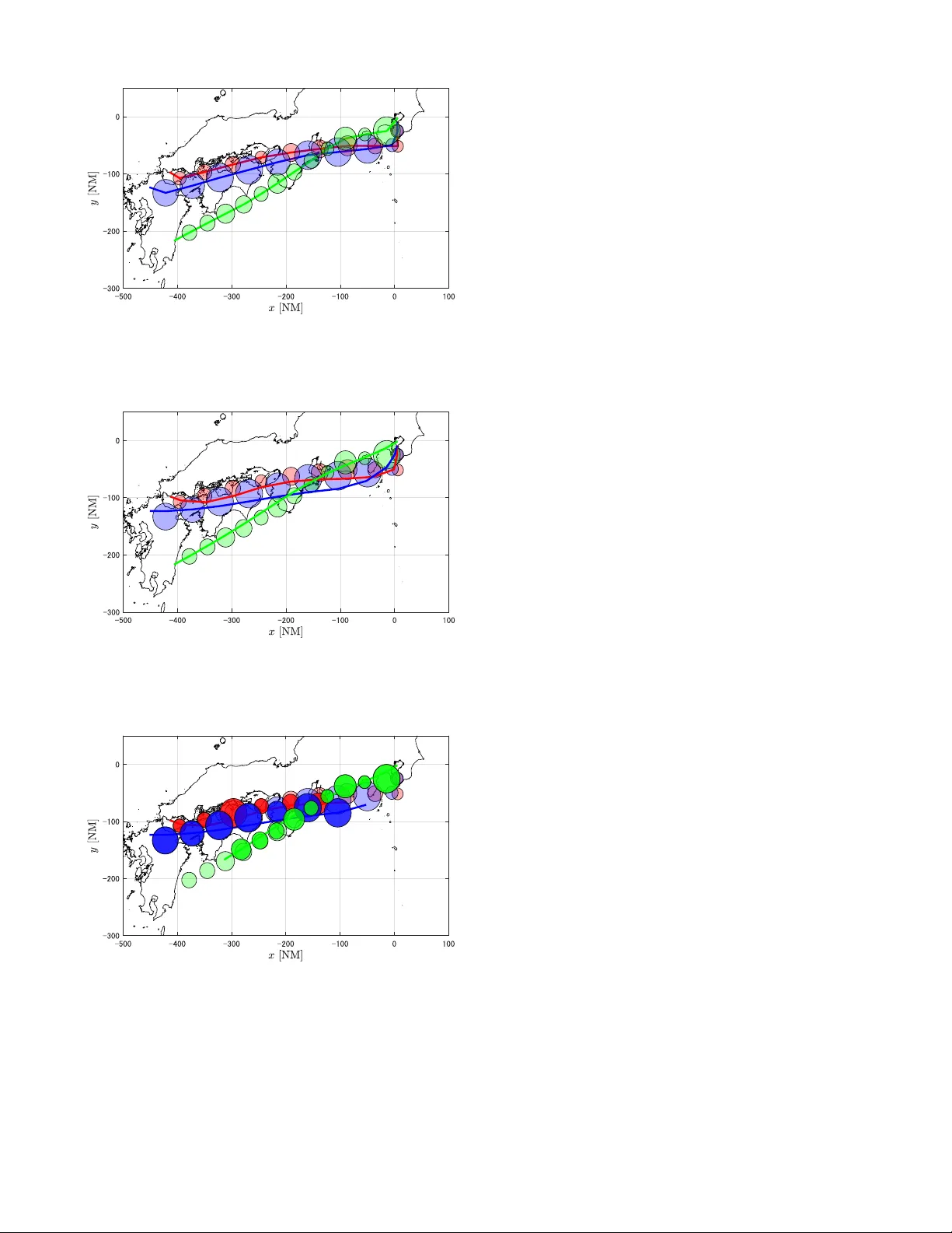
JOURNAL OF L A T E X CLASS FILES, VOL. 14, NO. 8, A UGUST 2015 1 T rajectory Planning of W eakly Supervised Aircraft Sho Y oshimura and Masaki Inoue, Member , IEEE Abstract —In this paper , we propose a novel framework of air traffic management (A TM). The framework is in particular char- acterized by the trajectory planning of weakly supervised air craft; the air traffic control (A TC) does not completely determine the trajectory of each aircraft unlike con ventional planning methods, but determines allow able safe sets of trajectories. A TC requests pilots to select their own trajectories fr om the sets, and the pilots determine ones by pursuing their own aims. For example, the selection can be based on pilot prefer ences and airline strategies. This tw o stage A TM system contrib utes to simultaneously achieve the both objectives of the A TC and pilots such as fuel cost minimization under safety management. The effectiv eness of the proposed A TM system is demonstrated in a simulation using actual air traffic data. Index T erms —T rajectory planning, air traffic management, optimization I . I N T RO D U C T I O N W ITH the gro wth of air traffic all over the world, air traffic management (A TM) systems need to be further dev eloped and to be operated more ef ficiently . As reported in [1], A TM is defined as dynamic and integrated management of air traffic and airspace through the provision of facilities and seamless services in collaboration with parties. In this paper , we focus only on control and management problems of aircraft trajectories from departure to arriv al. W e revie w the current A TM system and find its drawback. A sketch of the current system is given in Fig. 1. As illustrated in the figure, ov erall airspace is di vided to some smaller spaces. The current A TM is operated in a decentralized manner; in other words, a control task corresponding to each divided space is assigned to each air traffic control (A TC). Then, each A TC is responsible for safety of aircraft in an assigned space and manually designs aircraft trajectories. The design is based on positions of aircraft that are obtained from radar information. The trajectories designed by A TC are pro vided to pilots. A main limitation of the current A TM system lies in manually designing trajectories by A TC. W ith the growth of air traf fic, the number of aircraft contained in airspace increases. This increases burdens for the corresponding A TC, which inhibits ef ficient trajectory design. In addition, lack of communication between A TCs, caused by the traffic growth, can further deteriorate the efficiency . Therefore, a computer- aided and human-assist A TM system where overall airspace is managed in a centralized manner , is required. In the past two decades, various computer-aided methods of generating aircraft trajectories have been proposed [2]– [11]. One of the main topics is conflict avoidance. Please see, e.g., [5]–[10]. The conflict av oidance is in volv ed in S. Y oshimura and M. Inoue are with the Department of Applied Physics and Physico-Informatics, K eio University , Y okohama, Japan (e-mail: mi- noue@appi.keio.jp). optimal trajectory generation problems [5], [7]–[10]. In the current A TM system and pre vious works [3], [5]–[11], A TC determines aircraft trajectories completely and provides them to pilots. Pilots must obey the provided trajectories. The priority to A TC in trajectory determination plays a role for safety management of aircraft. In addition to the safety aim, A TC can achiev e to improve airport usage, e.g., by maximizing airport throughput. W e can say that the current A TM system meets aims of A TC. On the other hand, the priority to A TC may not be positi vely acceptable for pilots and airlines. Trajectories determined and enforced by A TC may be fuel-consuming or delayed ones, which are contrary to the aims of pilots and airlines. This paper addresses a novel A TM system design where trajectories are determined based on pilots and airlines aims in addition to safety constraints. T o sho w the feasibility of the A TM system design, we illustrate the existence of degree of freedom (DOF) in actual aircraft trajectories determined by A TC. Actual trajectories are depicted in Fig. 2, where trajectory data is extracted from CARA TS (Collaborativ e Actions for Renovation of Air T raffic Systems) Open Data 1 [12]–[15] on May 11, 2015. In the figure, the three solid lines represent actual trajectories. The translucent lines represent all trajectories where conflict av oidance is achiev ed. The DOF in trajectories, illustrated by the translucent lines, implies that the aims of pilots and airlines can be pursued in addition to safety constraints. Motiv ated from this fact, this paper studies a novel framew ork of A TM systems by utilizing this DOF in trajectory design. In this paper , we propose a frame work of A TM systems where A TC weakly supervises aircraft for the trajectories planning. An illustration of the proposed framew ork is shown in Fig. 3. In the A TM system, A TC designs allowable safe sets of aircraft trajectories, where conflict a voidance and other 1 CARA TS Open Data includes 3D-position and time data of all IFR (Instrument Flight Rules) commercial flights in Japanese airspace. Fig. 1: Illustration of the current A TM. Control tasks of aircraft from departure to arriv al are divided between airspace. For each airspace, an air traffic controller designs aircraft trajectories manually and provides them to pilots. JOURNAL OF L A T E X CLASS FILES, VOL. 14, NO. 8, A UGUST 2015 2 Fig. 2: Example of all trajectories that satisfy A TC require- ments including conflict av oidance. The three solid lines rep- resent actual trajectories. The translucent solid lines represent trajectories that avoid aircraft conflicts. Here, the conflict av oidance is defined that aircraft-aircraft distance is longer than 3 NM. Fig. 3: Illustration of the proposed A TM framework. In this figure, the black points represent the initial and terminal positions of the target aircraft. A TC designs an allowable safe set of trajectories which is represented by the red disks. A trajectory selected from the set by the pilot is represented by the blue cross marks. aims of A TC are achie ved, as depicted by red disks in the figure. Then, A TC requests pilots to select their trajectories from the sets. The selection can be based on pilot preferences or airline strategies. It is noted that for the trajectory selection, communication between pilots, such as cooperation, competi- tion and negotiation, is not required. Each pilot individually determines his/her trajectory by pursuing his/her own aims, e.g., by minimizing fuel costs or by reducing uncertainty of arriv al time in a decentralized manner . Designing trajectory-sets for aircraft has been also studied as flo w corridors, corridors-in-the-sky , or airspace tubes [16]– [19]. The concept of the corridor means an exclusi ve lane designed in airspace where autonomy is allo wed for each aircraft; each pilot can design his/her trajectory within the lane without instructions by A TC. This implies that the pilot must be responsible for av oiding an air miss or conflict with other aircraft by communicating with other pilots. This drawback is ov ercome in the proposed A TM system; each pilot needs not to address the conflict av oidance problem, but simply pursues his/her aims based on a giv en trajectory-set. The rest of this paper is organized as follows. In Section I I, the proposed frame work of A TM systems and problems of trajectory planning are briefly stated. In Section I I I, a trajectory design problem addressed by A TC is formulated as an optimization problem. By solving the problem, trajectory- sets that av oid aircraft conflicts are obtained. In Section I V , in a similar manner to Section I I I, a trajectory design problem addressed by pilots is formulated as an optimization problem. At the end of the section, the proposed A TM system is revie wed. In Section V , we sho w the ef fecti veness of the proposed system in a numerical simulation with CARA TS Open Data. I I . W E A K C O N T RO L I N A T M A. Outline of Pr oposed A TM In this subsection, we briefly show the outline of the proposed A TM system. The operation flow of the A TM system is given in Fig. 4. Operation of the A TM system is to control aircraft from departure to arri val. T rajectory planning runs recursiv ely at some time interval. For each trajectory planning, A TC designs allowable safe sets of trajectories, and then requests pilots to select their trajectories from the sets. The selection by pilots is performed independently of each other . This two-stage trajectory planning achie ves aims of pilots and airlines such as minimization of fuel consumption, while satisfying requirements by A TC such as conflict av oidance. Recall that the requests from A TC to pilots are gi ven by allowable safe sets of trajectories. The sets are utilized for pilots to minimize fuel costs based on detailed aircraft models and weather conditions. W e can say that in the proposed A TM system pilots are weakly supervised by A TC. The weakness contrib utes to separate A TC management and pilots optimization; in other words, safe management is performed independently of pilots choices. B. Pr oblem F ormulation Notation utilized in this paper is listed on T able I. In this subsection, problems of trajectory planning are briefly stated. Let N be the number of target aircraft considered in the problem. In this paper , trajectories refer to positions of aircraft at equal time intervals. T rajectories are restricted to two dimensions for simplicity , but they are easily extended to three dimensions. The position of aircraft i ∈ N := { 1 , . . . , N } at time k ∈ { 0 , 1 , . . . } is denoted by C i ( k ) := [ x i ( k ) y i ( k ) ] > . V ariables of aircraft are defined below . Let v i ( k ) , θ i ( k ) , u i ( k ) , and ψ i ( k ) be the speed, angle, speed difference, and angle difference of aircraft i at time k , respectively . The state of aircraft i at time k is denoted by X i ( k ) := [ C > i ( k ) v i ( k ) θ i ( k ) ] > . As stated abo ve, each trajectory planning is composed of two stages 1) trajectories design and request by A TC side and 2) trajectory design by pilots side. First, we focus on the design problem addressed by A TC as follows. W e assume that the initial time t i , the terminal time T i , the initial state X i ( t i ) , and the terminal state X i ( T i ) for all aircraft i ∈ N are gi ven. Then, A TC designs reference trajectory-sets W i ( k ) , k ∈ { t i + 1 , . . . , T i − 1 } , i ∈ N . Let W i ( k ) be a disk region. Then, the JOURNAL OF L A T E X CLASS FILES, VOL. 14, NO. 8, A UGUST 2015 3 A TC 1) Design ref eren ce trajectory - s et s Pil ot 2) Sele ct an trajectory fr om the set b y pu rsu in g ow n ai m  T raj ect ory planning  Operat ion Run recu rsive ly weak control Fig. 4: Operation flo w of the proposed A TM system. T rajectory planning runs recursively at some time interv al. A TC designs allowable safe sets of trajectories, and then requests them to the pilots. Pilots select trajectories from the sets independently of each other . The selections are based on their own aims. problem is reduced to a problem of finding the center C i ( k ) and radius r i ( k ) of W i ( k ) . In the remainder of this paper , W i ( k ) is described as W i ( k ) = { C i ( k ) , r i ( k ) } . Through the trajectory design, A TC pursues the following aims; • maximizing the DOF in the trajectory-set, defined by k r i k , • guaranteeing safety of aircraft by conflict avoidance. For simplification of notation, the set of time of aircraft i is denoted by T i ( t i ) := { t i + 1 , . . . , T i − 1 } . Letting r := [ r 1 · · · r N ] > , the trajectory design problem addressed by A TC is summarized as follows Problem 1. For giv en X i ( t i ) , X i ( T i ) , i ∈ N , find W i ( k ) , k ∈ T i ( t i ) , i ∈ N maximizing k r k subject to some constraints. Problem 1 corresponds to the design problem 1), which is illustrated in the operation flow of Fig. 4. Next, we briefly mention a trajectory design problem ad- dressed by pilots, which is solved next to Problem 1 . Each pilot solves the problem independently of each other . Assume that the initial state X i ( t i ) , the terminal state X i ( T i ) , the requested trajectory-set W i ( k ) , k ∈ T i ( t i ) , and disturbances d i ( k ) , k ∈ T i ( t i ) are gi ven. Then, each pilot selects a trajectory ˆ C i ( k ) , k ∈ T i ( t i ) by pursuing his/her aims, e.g., minimizing a fuel cost. The trajectory design problem addressed by a pilot labeled by i , is summarized as follo ws. Problem 2. For given X i ( t i ) , X i ( T i ) , W i ( k ) , k ∈ T i ( t i ) , find ˆ C i ( k ) , k ∈ T i ( t i ) minimizing some costs. Problem 2 corresponds to the design problem 2), which is illustrated in the operation flow of Fig. 4. Remark 1. It is assumed that model information of aircraft and a weather condition are av ailable for each pilot, while they T able I: Definition of variables of aircraft i in this paper . V ariables Description N number of target aircraft t i initial time T i terminal time W i reference trajectory-set (region defined as disk) C i center of W i , i.e., C i = [ x i , y i ] > r i radius of W i C sta ,i standard trajectory ∆ deviation between standard trajectory and center of region ˆ C i trajectory to be designed by pilot C pre ,i trajectory pilot select at the last trajectory planning d i disturbance x i x coordinate of position y i y coordinate of position v i speed θ i angle u i speed difference ψ i angle difference X i state, i.e., X i = [ C > i , v i , θ i ] > are not available for A TC. Precise model information and a weather condition play important role of reducing a fuel cost. Therefore, the pilot utilizes such information to solv e Problem 2 in an efficient manner and to reduce the achie vable cost. I I I . T R A J E C T O RY D E S I G N B Y A T C In this section, we mathematically formulate the trajectory design problem addressed by A TC. Problem 1 , which is briefly stated in Section I I, is re-formulated as an optimization problem. A. Cost Function In this subsection, cost functions of the trajectory design problem for A TC are defined. The decision v ariables are speed differences u := [ u 1 · · · u N ] > , angle differences ψ := [ ψ 1 · · · ψ N ] > , and radii r of all aircraft. Trajectory-sets to be designed are ev aluated by the size of r and the deviations from a standard trajectory C sta ,i ( k ) , k ∈ T i ( t i ) . The cost function to e valuate r is giv en by J 1 = − N X i =1 T i − 1 X k = t i +1 ln ( r i ( k ) + ε ) , (1) where ε is a positiv e constant. This role of ε is to prev ent div ergence of J 1 . In addition, the cost function to e valuate the deviations is gi ven by J 2 = N X i =1 T i − 1 X k = t i +1 ∆ i ( k ) 2 + N X i =1 T i − 2 X k = t i +1 (∆ i ( k + 1) − ∆ i ( k )) 2 , (2) where ∆ i ( k ) = C i ( k ) − C sta ,i ( k ) . The role of the second term is to prev ent a large angle change in one time step. By this J 2 , we aim at generating realistic trajectories, while av oiding impractical ones. Then, the cost function utilized in the problem here is defined by J A TC ( u, ψ , r ) := J 1 + αJ 2 , (3) JOURNAL OF L A T E X CLASS FILES, VOL. 14, NO. 8, A UGUST 2015 4 where α is a non-negati ve constant. Remark 2. There is another candidate of the cost function J 1 for ev aluating the radii r i . For example, ln ( r i ( k ) + ε ) in (1) can be replaced by 1 / ( r i ( k ) + ε ) 2 . In this paper , numerically tractable J 1 , gi ven by (1), is considered. B. Constr aints W e gi ve constraints deri ved from physical properties of aircraft, from A TM system requirements, and for A TM system operation. First, the constraints deriv ed from the physical properties are given as follows. • Aircraft dynamics Assume that the dynamics of all the target aircraft are the same. The dynamics of each aircraft is described by     x i ( k + 1) y i ( k + 1) v i ( k + 1) θ i ( k + 1)     = f         x i ( k ) y i ( k ) v i ( k ) θ i ( k )         +     0 0 u i ( k ) ψ i ( k )     , (4) where f is giv en by f         x i ( k ) y i ( k ) v i ( k ) θ i ( k )         :=     x i ( k ) + v i ( k ) cos θ i ( k ) y i ( k ) + v i ( k ) sin θ i ( k ) v i ( k ) θ i ( k )     . (5) Here, recall that u i ( k ) and ψ i ( k ) are speed difference and angle difference at time k ∈ T i ( t i ) of aircraft i ∈ N . In the model (4), they are the control input to aircraft. • Angular difference Angular dif ference of each aircraft trajectory , denoted by ψ i ( k ) , is restricted as follo ws. − Ψ ≤ ψ i ( k ) ≤ Ψ , ∀ k ∈ T i ( t i ) , ∀ i ∈ N , (6) where Ψ is the maximum angle dif ference of a trajectory . • Speed difference Speed difference of each aircraft trajectory , denoted by u i ( k ) , is restricted as follo ws. − U ≤ u i ( k ) ≤ U, ∀ k ∈ T i ( t i ) , ∀ i ∈ N , (7) where U is the maximum speed dif ference to be applied. • Speed Speed of each aircraft, denoted by v i ( k ) , is restricted as follows. V min ≤ v i ( k ) ≤ V max , ∀ k ∈ T i ( t i ) , ∀ i ∈ N , (8) where V min and V max are the lo wer and upper bounds of v i ( k ) . Next, the constraints related to A TM system requirements are giv en as follo ws. • T erminal constraint Constraints on the speed and angle at the terminal time T i are gi ven. The deviation between the speed at T i and the reference V ter is less than or equal to δ v , and the deviation between angle at T i and the reference Θ ter is less than or equal to δ θ . They are described by − δ v ≤ v i ( T i ) − V ter ≤ δ v , ∀ i ∈ N , (9) − δ θ ≤ θ i ( T i ) − Θ ter ≤ δ θ , ∀ i ∈ N . (10) • Constraint for conflict av oidance A constraint for conflict av oidance is giv en by k C i ( k ) − C j ( k ) k − ( r i ( k ) + r j ( k )) ≥ D, (11) ∀ k ∈ {T i ( t i ) ∩ T j ( t j ) } , ∀ i 6 = j ∈ N , where D is a positive constant. W e illustrate the meaning of (11) with Fig. 5. The left side of (11) represents the allow able minimum distance between two aircraft, which is illustrated in Fig. 5. Therefore, D plays a role of a safety margin. • Constraint for feasibility In this paper , feasibility means that the trajectory design problem performed by pilots are feasible. In other w ords, ev ery pilot can select a trajectory from a trajectory-set requested by A TC. This is described as k C i ( k + 1) − C i ( k ) k − ( r i ( k + 1) + r i ( k )) ≥ V min , ∀ k ∈ { t i ∪ T i } , ∀ i ∈ N , (12) k C i ( k + 1) − C i ( k ) k + ( r i ( k + 1) + r i ( k )) ≤ V max , ∀ k ∈ { t i ∪ T i } , ∀ i ∈ N , (13) where r i ( t i ) = 0 and r i ( T i ) = 0 , i ∈ N . W e illustrate the meaning of (12) and (13) with Fig. 6. Equation (12) means that the minimum distance of every pair of adjacent regions is longer than or equal to the realizable minimum distance, i.e., the trajectory is realized for some u i , ψ i , v i , θ i , x i , and y i satisfying (4)-(11). In a similar manner , equation (13) means the maximum distance of ev ery pair of adjacent regions is shorter than or equal to the realizable maximum distance. Finally , a constraint for A TM system operation is giv en. • Operation Constraint W e define a constraint that works at re-planning of trajec- tories. Consider that a trajectory planning is performed at a time k = t i . Then, we suppose that pilots select ˆ C i ( k ) , k ∈ T i ( t i ) . It should be noted that all the future trajectories ˆ C i ( t i + 1) to ˆ C i ( T i − 1) are selected by pilots i ∈ N based on their aims. At the re-planning, we incorporate the aims into trajectories to be redesigned by A TC. Let us consider that trajectories are re-planed at a time t i + τ , where τ ∈ { 1 , 2 , . . . , T i − 2 − t i } . Then, we need to impose a constraint on trajectories redesigned by A TC. W e let C pre ,i ( k ) = ˆ C i ( k ) , k ∈ T i ( t i ) . Then, trajectory-sets W i ( k ) , k ∈ { t i + τ +1 , . . . , T i − 1 } to be re- designed must include the last selection C pre ,i ( t i + τ + 1) to C pre ,i ( T i − 1) such that pilots can select the same best trajectories. This constraint is described by a condition on C i ( k ) and r i ( k ) to be redesigned as k C pre ,i ( k ) − C i ( k ) k ≤ r i ( k ) , ∀ k ∈ T i ( t i + τ i ) , ∀ i ∈ N . (14) The meaning of the equation is illustrated in Fig. 7. JOURNAL OF L A T E X CLASS FILES, VOL. 14, NO. 8, A UGUST 2015 5 T im e: Aircr aft: Mi nim um D ist ance A ircr af t: T im e: Fig. 5: Constraint for conflict avoidance. The minimum dis- tance between the aircraft i and j at time k , which is described by the left side of (11), is sho wn. Mi nim um D ist ance M axim um Dist ance T im e: T im e: Fig. 6: Constraints for feasibility . The minimum and maxmum distance of adjacent regions at time k and k + 1 , which are described by the left side of (12) and (13), respecti vely , are shown. C. Optimization Pr oblem Problem 1 , which is stated in Section I I, is mathematically formulated in this subsection. T o this end, we let X := [ X > 1 X > 2 · · · X > N ] > . Then, the optimization problem addressed by A TC is summarized as follows. Problem 3. For giv en X i ( t i ) , X i ( T i ) , C pre ,i ( k ) , k ∈ T i ( t i ) , i ∈ N , minimize u,ψ ,r ,X J A TC ( u, ψ , r ) (15) sub ject to Eqs . (4) − (14) . In the following, the optimizer to Problem 3 is denoted by ( u ∗ , ψ ∗ , r ∗ , X ∗ ) . A trajectory-set W ∗ i ( k ) , k ∈ T i ( t i ) is obtained based on the solution to Problem 3 . Then, W ∗ i ( k ) , k ∈ T i ( t i ) is provided to each pilot. Remark 3. Note again that Problem 3 is formulated with- out utilizing information on detailed aircraft dynamics and weather conditions. This is because that such information is not necessary for system management including the con- flict avoidance. On the other hand, the information can be efficiently utilized by pilots, e.g., for reducing fuel costs. The optimization problem addressed by pilots utilizes aircraft models based on B AD A data [20] or weather situation based on global forecasting systems, e.g., GDPFS (The Global Data- Processing and Forecasting System) [21]. Remark 4. In this paper, a DOF in trajectories is expressed by spatial regions, denoted by W i ( k ) = { C i ( k ) , r i ( k ) } . It should be emphasized that the spatial DOF is equiv alently T im e: Aircr aft: T im e: t he trajectory sel ect ed by p il ot 𝑖 at the la st plann ing Fig. 7: Operation constraint. The trajectory C pre ,i , which is selected at the last planning, must be included in W i , which is redesigned by A TC at the current planning. The trajectory C pre ,i is represented by the blue solid line, while the regions W i is represented by the red disks. T ransf orma ble DO F in spat ial dom ain Ba ll r egion DO F in ti m e dom ain Disk reg ion Fig. 8: Spatial DOF and temporal DOF . A spatial DOF is a spatial ball region where an aircraft must be included at a specified time . A temporal DOF is a time range at any of which an aircraft must pass a vertically-placed disk. transformed into temporal one. As studied abo ve, a spatial DOF in trajectories is expressed by a spatial ball region that aircraft must be included at a specified time k . On the other hand, a temporal DOF is expressed by a time range at any of whic h aircraft passes a specified v ertically-placed disk. The expressions are illustrated in Fig. 8. The two expressions of DOF are equiv alent each other . Remark 5. Since Problem 3 is in the class of high- dimensional nonlinear optimization problems, the choice of initial v alues of decision v ariables is essential to obtain a better local optimum. In this paper , the initial guess of u and ψ is determined based on standard trajectories. Otherwise, at re- planning case, the initial guess of C i ( k ) , k ∈ T i ( t i ) is based on pilots selections C pre ( k ) , k ∈ T i ( t i ) , which are designed at the last planning. I V . T R A J E C T O RY D E S I G N B Y P I L O T S In Section I I I, the trajectory design problem addressed by A TC is formulated. In Section I V , we focus on a trajectory design problem addressed by pilots . In the design problem of JOURNAL OF L A T E X CLASS FILES, VOL. 14, NO. 8, A UGUST 2015 6 this section, we focus only on a pilot labeled by i ∈ N . It is assumed that the reference trajectory-set, denoted by W ∗ i ( k ) , k ∈ T i ( t i ) , is gi ven and available for the design problem. Then, in a similar manner to the A TC case, the design problem by the pilot is formulated as an optimization problem. In this section, all decision variables of the optimization problem are denoted as ˆ · in order to distinguish them from those in Problem 3 . A. Cost Function The cost function to ev aluate the aims of the pilot is given. The decision v ariables are speed difference ˆ u i and angular difference ˆ ψ i . The cost function is described by J pilot ( ˆ u i , ˆ ψ i ) := T i − 2 X k = t i    ˆ u i ( k ) U  2 + ˆ ψ i ( k ) Ψ ! 2   . (16) This cost function J pilot ev aluates fuel costs of aircraft labeled by i ∈ N . The fuel costs are defined as a sum of squared control inputs of aircraft based on the definition of the work [11]. In (16), variables ˆ u i and ˆ ψ i are normalized such that the effects of them are fairly ev aluated. B. Constr aints Constraints that come from physical properties of aircraft and from A TM system requirements are listed. Constraints from aircraft specification are the same as (6)-(8), while those from aircraft dynamics are more precise than (4). W e assume that information of disturbance d , which represents, e.g., wind condition of airspace, is av ailable for trajectory design by the pilot. Then, aircraft dynamics are modified from (4) to     ˆ x i ( k + 1) ˆ y i ( k + 1) ˆ v i ( k + 1) ˆ θ i ( k + 1)     = f         ˆ x i ( k ) ˆ y i ( k ) ˆ v i ( k ) ˆ θ i ( k )         +     0 0 ˆ u i ( k ) ˆ ψ i ( k )     +     d x,i ( k ) d y ,i ( k ) 0 0     . (17) In this problem setting, disturbances d i ( k ) are only ap- plied to aircraft positions, in other words, d i ( k ) = [ d x,i ( k ) d y ,i ( k ) 0 0 ] > holds. For constraints from A TM system requirements, in addition to (9) and (10) each pilot selects his/her own trajectory from the trajectory set, which is designed and requested by A TC. Recall here that an aircraft trajectory to be designed by the pilot is denoted by ˆ C i ( k ) and that the trajectory-set designed by A TC is denoted by W ∗ i ( k ) = { C ∗ i ( k ) , r ∗ i ( k ) } . Then, the constraint on the trajectory selection is described by r ∗ i ( k ) ≥ k C ∗ i ( k ) − ˆ C i ( k ) k 2 , ∀ k ∈ T i ( t i ) . (18) C. Optimization Pr oblem The optimization problem addressed by each pilot is sum- marized as follows. Problem 4. F or giv en X ∗ i ( t i ) , X ∗ i ( T i ) , W ∗ i ( k ) , k ∈ T i ( t i ) , minimize ˆ u i , ˆ ψ i , ˆ X i J pilot ( ˆ u i , ˆ ψ i ) (19) sub ject to Eqs . (5) − (10) , (17) , (18) . Glo b al Co n troller Pilo t Aircraf t … …  Pr ob le m 4 Sele ct an tra je ct ory from the set  Pr oblem 3 Design ref ere nce tra je ct ory - sets A TC Fig. 9: Operation flo w of the proposed A TM system. T rajectory planning runs recursi vely at some time interv al. In one trajec- tory planning, trajectory design is performed sequentially by A TC and pilots. Trajectory-sets and trajectories are determined based on the solutions to Problem 3 and 4 , respectively . In the following, the optimizer to Problem 4 is denoted by ( ˆ u † i , ˆ ψ † i , ˆ X † i ) . Then, the optimal trajectory is denoted by ˆ C † i ( k ) , k ∈ T i ( t i ) . Remark 6. In this paper , no precise model of aircraft dynam- ics is utilized ev en in Problem 4 . In a practical setting, (17) need to be replaced by a more precise model. Utilizing more detailed aircraft dynamics, the problem is formulated in the same manner . The whole operation flo w of the proposed A TM system is revie wed. The block diagram shown as Fig. 9 illustrates a more detailed operation flow than that of Fig. 4. Each trajectory planning is composed of two stages; 1) trajectory- set design by A TC and 2) trajectory design by pilots. 1) A TC designs trajectory-sets by solving Pr oblem 3 . In the problem setting of Problem 3 , giv en initial states X i ( t i ) , terminal states X i ( T i ) , trajectories selected by pilots at the last trajectory planning, denoted by C pre ,i ( k ) , k ∈ T i ( t i ) , i ∈ N , we aim at finding reference trajectory-sets W i ( k ) , k ∈ T i ( t i ) . A TC requests pilots to select their trajectories from the designed sets W ∗ i ( k ) , k ∈ T i ( t i ) . 2) Then, each pilot design his/her trajectory by solving Problem 4 independently of each other . In the problem setting of Pr oblem 4 , gi ven X ∗ i ( t i ) , X ∗ i ( T i ) , i ∈ N , we aim at finding trajectories ˆ C i ( k ) , k ∈ T i ( t i ) . If re-planning is required due to some real-world uncertainties, we let C pre ,i ( k ) = ˆ C † i ( k ) , k ∈ T i ( t i ) . Then, the two stage design is performed again. V . N U M E R I C A L S I M U L A T I O N S W e verify the effecti veness of the proposed A TM system, including aircraft trajectory design, in a numerical simulation. T o this end, the proposed design method is applied to actual data extracted from CARA TS Open Data. The data includes three trajectories from or arriv e at HANED A airport on May 11, 2015. These trajectories are illustrated in Fig. 10. In the figure, HANED A airport is located at the origin. The aircraft trajectories that depart from HANED A are represented by red and blue solid lines, while that arriv es at HANEDA is represented by the green solid line. JOURNAL OF L A T E X CLASS FILES, VOL. 14, NO. 8, A UGUST 2015 7 Fig. 10: Actual trajectories are extracted from CARA TS Open Data. The aircraft trajectory that departs from HANED A is represented by red and blue solid lines, while that arrives at HANED A is represented by the green solid line. A. Simulation Conditions In the simulation, trajectory planning runs at the initial time and middle time of the operation. At the middle time, only trajectory design by A TC is demonstrated in this section. Conditions on the first and second trajectory planning are giv en below . Conditions on the first trajectory planning are giv en. For each aircraft i ∈ N = { 1 , 2 , 3 } , the initial operation time t i , the terminal operation time T i , the initial state X i ( t i ) , and the terminal state X i ( T i ) are given as follows. • Aircraft 1 t 1 = 1 , T 1 = 12 , X 1 ( t 1 ) = [ 4 . 71 − 8 . 42 16 . 4 − 1 . 58 ] > X 1 ( T 1 ) = [ − 413 − 97 . 5 22 . 2 2 . 63 ] > • Aircraft 2 t 2 = 2 , T 2 = 13 , X 2 ( t 2 ) = [ 4 . 50 − 9 . 01 17 . 7 − 1 . 56 ] > X 2 ( T 2 ) = [ − 452 − 123 31 . 1 2 . 84 ] > • Aircraft 3 t 3 = 2 , T 3 = 15 , X 3 ( t 3 ) = [ − 406 − 217 31 . 8 0 . 471 ] > X 3 ( T 3 ) = [ 5 . 91 − 1 . 96 31 . 2 0 . 833 ] > Here, one time step corresponds to six minutes. In the cost function (3), the parameter is chosen by α = 0 . 01 . T o solve Problem 3 , the initial values of u and ψ are computed based on the standard trajectories in actual data, while that of r is zero. In Pr oblem 4 , for simplicity , we suppose that the wind disturbance d is constant and that the magnitude and angle of d are 1 / 3 and π / 4 , respectiv ely . That is, d x,i ( k ) = 0 . 236 , d y ,i ( k ) = 0 . 236 , k ∈ T i , i ∈ N . Note that only pilots utilize this wind condition. T o solve Problem 4 , the initial values of ˆ u and ˆ ψ are determined such that the center of the trajectory-sets requested by A TC are tracked. Conditions on the second trajectory planning are gi ven. The second trajectory planning is carried out at the fifth time step, i.e., t i = 5 , i ∈ N . The parameter α of (3) is fixed as α = 0 . 01 , which is the same as the first planning. T o solve the T able II: Comparison at the resulting DOF , defined by k r ( k ) k , at the first trajectory planning. Aircraft 1 Aircraft 2 Aircraft 3 Mean 13 . 5 21 . 6 15 . 5 Standard deviation 2 . 30 5 . 65 3 . 85 T able III: Comparison at the values of (16) as fuel costs. Aircraft 1 Aircraft 2 Aircraft 3 total T rajectory A 2 . 91 1 . 95 0 . 44 5 . 31 T rajectory B 2 . 99 2 . 07 0 . 47 5 . 44 T rajectory C 2 . 13 1 . 62 0 . 25 4 . 00 problem, the initial values of ˆ u and ˆ ψ are the same as ones selected by pilots at the first trajectory planning. In addition, the initial value of ˆ r is zero. B. Results The resulting trajectories of the first trajectory planning are sho wn in Figs. 11 and 12. Figure 11 shows the result of the trajectory design by A TC. In the figure, the reference trajectory-sets are represented by the red, blue, and green disks, while the trajectories that track the center of the sets are represented by the solid lines. The mean and standard deviation of the resulting r i ( k ) , which is the DOF , are listed on T able II. The DOFs of Aircraft 1 and Aircraft 2, which are adjoining, are the minimum and maximum one. This is because that the cost tends to be small when one DOF in adjoining trajectories is big and the other is small. Figure 12 shows the result of the trajectory designed by pilots. In the figure, the trajectories selected by pilots are represented by the red, blue, and green solid lines. W e see that all the trajectories are included in the trajectory-sets requested by A TC, which are represented by the disks. This implies that conflict av oidance is achieved. The trajectories are quantitativ ely ev aluated by the cost function J pilot , which is defined in (16) and simulates fuel costs in some sense. The cost values of actual trajectories (Trajectory A), trajectories that track the center of the sets (T rajectory B), and the trajectories selected by pilots (T rajectory C) are listed on T able III. This shows that the fuel costs of T rajectory C is the minimum for all aircraft. This result implies that although only a simple aircraft model and a performance index of fuel costs are used in this simulation, it is expected that performances are improved ev en when more detailed models and performance indexes are used. Figure 13 shows the result of the second trajectory planning. In the figure, the reference trajectory-sets redesigned by A TC are drawn on Fig. 12. The sets are represented by the deep red, blue, and green disks. It is confirmed that the constraint for operation is satisfied; the trajectories selected by pilots at the first trajectory planning are included in the trajectory-sets redesigned by A TC. This implies that each pilot can choose the same trajectory as the last planning if there is no update for the weather condition and pilots and airlines cannot receiv e demerits by the re-planning. JOURNAL OF L A T E X CLASS FILES, VOL. 14, NO. 8, A UGUST 2015 8 Fig. 11: Result of A TC design at the first trajectory planning. The sets designed by A TC are represented by red, blue, and green disks. Center of the disks is connected and represented by the solid lines. Fig. 12: Result of pilots design at the first trajectory planning. The trajectories selected by pilots are represented by the solid lines. The red, blue, and green disks are the sets designed and requested by A TC, which are the same as those of Fig. 11. Fig. 13: Result of A TC re-design at the second trajectory planning. The sets redesigned by A TC are represented by deep red, blue, and green disks. The trajectories selected by pilots at the first trajectory planning are represented by the solid lines. V I . C O N C L U S I O N In this paper, we proposed a nov el framework of A TM systems where A TC weakly supervises aircraft. Aircraft tra- jectories, which are completely determined by A TC con ven- tionally , are designed by A TC as trajectory-sets , and the sets are provided to pilots. Then, the pilots indi vidually select their trajectories from the sets. W e sho wed that both the safety requirement, which is the aim of A TC, and reduction of fuel consumption, which is the aim of pilots and airlines, were achiev ed in the A TM system. The authors expect that the pro- posed A TM system may not be directly implemented to real- world A TM. Howe ver , the essence of the weak supervision, i.e., idea of explicitly providing DOFs to pilots, can be utilized to practical A TM systems in a modified manner . The optimization problems formulated for trajectory plan- ning are nonlinear to some decision variables, which are numerically intractable. In future work, we need to reformulate them to more tractable ones. A C K N O W L E D G M E N T This work was supported by Grant for Basic Science Research Projects from Sumitomo Foundation and by Grant- in-Aid for Scientific Research (A), No. 18H03774 from JSPS. R E F E R E N C E S [1] International Civil A viation Organization, “Global Air T raffic Manage- ment Operational Concept, ” Doc 9854, 2005. [2] Y . Miyazawa, N. K. W ickramasinghe, A. Harada, and Y . Miyamoto, “Dynamic programming application to airliner four dimensional optimal flight trajectory , ” in Proceedings of AIAA Guidance, Navigation, and Contr ol Conference , 2013. [3] L. Pallottino, E. M. Feron, and A. Bicchi, “Conflict resolution problems for air traffic management systems solved with mixed inte ger program- ming, ” IEEE T r ansactions on Intelligent T ransportation Systems , vol. 3, no. 1, pp. 3–11, 2002. [4] P . Bonami, A. Olivares, M. Soler , and E. Staffetti, “Multiphase mixed- integer optimal control approach to aircraft trajectory optimization, ” Journal of Guidance, Contr ol, and Dynamics , vol. 36, no. 5, pp. 1267– 1277, 2013. [5] P . Menon, G. Sweriduk, and B. Sridhar , “Optimal strategies for free- flight air traf fic conflict resolution, ” Journal of Guidance, Contr ol, and Dynamics , vol. 22, no. 2, pp. 202–211, 1999. [6] Y .-x. Han, X.-q. Huang, and Y . Zhang, “T raffic system operation opti- mization incorporating buffer size, ” Aer ospace Science and T echnology , vol. 66, pp. 262–273, 2017. [7] X.-M. T ang, P . Chen, and B. Li, “Optimal air route flight conflict resolution based on receding horizon control, ” Aerospace Science and T echnology , vol. 50, pp. 77–87, 2016. [8] A. E. V ela, S. Solak, J.-P . B. Clarke, W . E. Singhose, E. R. Barnes, and E. L. Johnson, “Near real-time fuel-optimal en route conflict resolution, ” IEEE T ransactions on Intellig ent Tr ansportation Systems , v ol. 11, no. 4, pp. 826–837, 2010. [9] J. Hu, M. Prandini, and S. Sastry , “Optimal coordinated maneuvers for three-dimensional aircraft conflict resolution, ” Journal of Guidance , Contr ol, and Dynamics , v ol. 25, no. 5, pp. 888–900, 2002. [10] A. Bicchi and L. Pallottino, “On optimal cooperative conflict resolution for air traffic management systems, ” IEEE T ransactions on Intelligent T ransportation Systems , pp. 221–231, 2000. [11] D. T oratani and E. Itoh, “Ef fects on optimal mer ging trajectories with allocation optimization from the trade-off between fuel consumption and flight time, ” SICE J ournal of Control, Measurement, and System Inte gration , vol. 11, no. 3, pp. 182–189, 2018. [12] Ministry of Land, Infrastructure, Transport and T ourism (MLIT), Study Group for the Future Air T raffic Systems, “Long-term V ision for the Future Air T raffic Systems-Changes to Intelligent Air Traf fic Systems, ” 2010. [13] H. Matsuda, A. Harada, T . Kozuka, Y . Miyazawa, and N. K. Wickramas- inghe, “ Arriv al time assignment by dynamic programming optimization, ” in Air T raf fic Management and Systems II . Springer , 2017, pp. 185–204. [14] Y . Fukuda, M. Oka, N. K. Wick, K. Uejima et al. , “ Air traffic open data and its impro vement, ” in Proceedings of Asia-P acific International Symposium on Aerospace T echnology . Engineers Australia, 2015. JOURNAL OF L A T E X CLASS FILES, VOL. 14, NO. 8, A UGUST 2015 9 [15] N. K. W ickramasinghe, M. Brown, H. Hirabayashi, and S. Nagaoka, “Feasibility study on constrained optimal trajectory application in the japanese airspace, ” in Proceedings of AIAA Modeling and Simulation T echnologies Confer ence , 2017. [16] R. Hof fman and J. Prete, “Principles of airspace tube design for dynamic airspace configuration, ” in Pr oceedings of the 26th Congr ess of ICAS and 8th AIAA ATIO , 2008. [17] N. T akeichi and Y . Abumi, “Benefit optimization and operational re- quirement of flow corridor in japanese airspace, ” Proceedings of the Institution of Mechanical Engineers, P art G: Journal of Aer ospace Engineering , vol. 230, no. 9, pp. 1780–1787, 2016. [18] M. Xue, “Design analysis of corridors-in-the-sky , ” in Proceedings of AIAA Guidance, Navigation, and Contr ol Confer ence , 2009. [19] A. Y ousefi and A. N. Zadeh, “Dynamic allocation and benefit assessment of ne xtgen flo w corridors, ” T ransportation Researc h P art C: Emerging T echnologies , vol. 33, pp. 297–310, 2013. [20] A. Nuic, D. Poles, and V . Mouillet, “BAD A: An advanced aircraft performance model for present and future A TM systems, ” International Journal of Adaptive Contr ol and Signal Pr ocessing , v ol. 24, no. 10, pp. 850–866, 2010. [21] WMO, “Global data-processing and forecast- ing system, ” https://public.wmo.int/en/programmes/ global- data- processing- and- forecasting- system. PLA CE PHO TO HERE Sho Y oshimura Sho Y oshimura was born in Chiba, Japan in 1993. He received the Bachelor’ s degree in Engineering from K eio Univ ersity in 2017. He is currently a Master Course student in Keio Uni ver- sity . His research interests include air traffic manage- ment design and system identification for large-scale systems. PLA CE PHO TO HERE Masaki Inoue Masaki Inoue was born in Aichi, Japan, in 1986. He receiv ed the M.E. and Ph.D. de- grees in engineering from Osaka Univ ersity in 2009 and 2012, respectively . He served as a Research Fellow of the Japan Society for the Promotion of Science from 2010 to 2012. From 2012 to 2014, He w as a Project Researcher of FIRST , Aihara Innov ative Mathematical Modelling Project, and also a Doctoral Researcher of the Graduate School of Information Science and Engineering, T okyo Insti- tute of T echnology . Currently , he is an Assistant Professor of the Faculty of Science and T echnology , Keio University . His research interests include stability theory of dynamical systems. He received sev eral research awards including the Best Paper A wards from SICE in 2013, 2015, and 2018, from ISCIE in 2014, from IEEJ in 2017, and the T akeda Best Paper A ward from SICE in 2018. He is a member of IEEE, SICE, ISCIE, and IEEJ.