Adaptive Control for Marine Vessels Against Harsh Environmental Variation

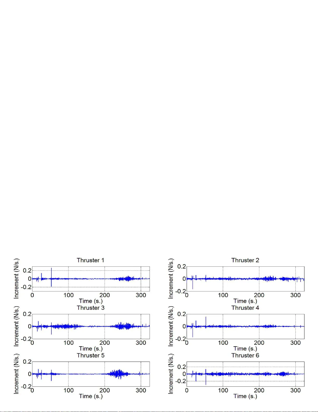
IEEE TRANSACTIONS ON SYSTEMS, MAN, AND CYBERNETICS: SYSTEMS, V OL. X, NO. X, X 2017 1 Adapti v e Control for Marine V essels Against Harsh En vir onmental V aria tion Fangwen T u, Shuzhi Sam Ge, F ellow , IEEE, Y oo Sang C h oo, a n d Chang Chieh Han g , F ellow , IEEE Abstract —In this paper , robust c ontrol with sea state obser ver and dynamic thrust allocation is p roposed fo r th e Dynamic Positioning (DP) of an accommodation vessel in th e presence of unknown hydrodynamic for ce variation and the inp ut time delay . In order to ov ercome the huge f or ce v ariation due to the adjoining Floating Production Storage and Offloading (FPS O) and accommodation vessel, a n ov el sea state obser ver is designed. The sea observe r can effectively monitor the variation of the drift wa ve-induced for ce on the vessel and activa te Neural Network (NN) compensator in the controller when large wa ve f orce is identified. Moreov er , the wi nd drag coefficien ts can be adaptively approximated in t he sea observ er so that a feedforward control can be achieved. Based on this, a robust constrained control is deve loped to guarantee a safe operation. The time delay inside the control in put is also considered. Dynamic th rust allocation module is presented to distribute the generalized control in put among azimuth thrusters. Under the proposed sea observe r and control, the b ou n dedness of all the closed-loop signals are demonstrated via rigor ous L yapun ov analysis. A set of simulation studies are condu cted to verify the effectiveness of the proposed control scheme. Index T erms —Dynamic positioni ng, sea state observer , robust constrained control, input delay , dynamic thrust allocation, deep water techn ology I . I N T RO D U C T I O N FPSOs unit are high ly de m anded to prod uce, pro cess hy- drocarb ons and store oil in marin e industry . At the same time, Accommo d ation V essels (A V) which can p rovide the s pace f or logistic supp ort and open dec k space in deep sea en vironm ent is n eeded to han dle the maintenan ce related work offshore. In this way , these A Vs must ensure co nnected for con tinuous personn e l and equip ments transfer th r ough gang way . Thus, the motiv ation of this p aper is to design a DP system to allow the A Vs to maintain proper relativ e position an d heading under varying environmental situatio ns. One of the most significant phenomena dur in g the operation is the hyd r odyna m ic interaction between the two vessels. This strong influence is called shieldin g effect [1] wh ich results in huge en vironm ental force variation. The ocean wa ves can propag ate in mu ltip le dir e ctions. Once the smaller a c commo- dation vessel situates in the downstream shadow of FPSO as shown in Fig. 1 , the large FPSO would pro tect the sm a ller vessel in the v icinity . Co n sequently , the vessel only receives small wa ve-induced for ce. Whe n the vessel m oves out of the shadow , the environmental loads on the A V would in crease. Thus, it is a very challenging to keep a fixed relativ e position and headin g und er this variation. In order to alarm th e it, for the first time, a novel sea state ob server is pro p osed. The ob ser ver is motiv ated b y the fault d ia g nosis proc ess in fault toleran t contr o l [2] [3]. Different from trad itional fault observer, the sea state observer is able to adaptively estimate the wind force an d mo ment. The estimated force an d mo ment is used for a f e e dforward control to counteract the wind effect on the vessel. Based on this, the detection o f the shieldin g effect is n ot only judg ed b y th e residu al be twe e n actual system states and estimated states, but, th e estimated wind drag co efficients are selected as th e ind icator of the shielding effect due t o the over-estimation phenomena. After huge w av e- induced for ce a n d momen t ar e detected, NNs are applied in both sea observer and controller to compen sate the wa ve force . Additionally , to en sure the extended length of gangway Fig. 1. Definition of the coordinate system between an A V and the FPSO no t exceed the limit stroke, the trackin g err ors must b e regulated. I n [4], Barrier L ya- punov Function (BLF) method was propo sed to handle ou t- put constraint. Compared to oth e r sche m es, BLF needs less restrictiv e initial co n ditions and doe s not require the explicit system solutio n. A general framework to hand le the pr escribed perfor mance tracking problem f or strict fee d back systems were propo sed in [ 5]. Apa r t from tracking erro r constra in t, the input delay existing in the tr usters can severely degrade th e control performance . Th e de la y is mainly caused by the long response time of the thruster driver [6]. Thus, it is necessary to take the in put delay into con sideration for the contr ol design. Much resear ch has been d one to cope with inpu t delay for linear system [7] [8]. Howe ver , the nonlin earity of the vessel systems bring mo re challenges to the co ntrol design. In [9] [10], an adaptive tracking control scheme has been developed for a class of multi- in put and mu lti- o utput (MI MO) no nlinear system with inp ut delay . A vir tual observer is constru cted as an au xiliary system to con vert the inpu t delay system into IEEE TRANSACTIONS ON SYSTEM S, M AN, AND CYBERNE T ICS: SYSTEM S, VOL. X, NO. X, X 2017 2 a non -delayed one. A robust saturation contr o l approa c h for vibration s uppre ssion of b uilding s tructure s with input d elay is presented in [11]. This co ntrol is able to han dle bo unded tim e- varying inpu t delay . But integrating tracking erro r con straint with inp ut delay is seldom studied, e sp ecially for nonlinear systems. Ther e fore, in this paper, in or der to gu arantee a smooth and safe op eration, both of these two requ irements need to be considered simultaneously . In this pa p er , we consider an A V with 6 azim uth thrusters which can p roduc e forces in all dir ections. The aim of thrust allocation mo dule is to d istribute the de sire d contro l effort among the trusters, i.e., to solve the required ro tation an gle and output thrust for each thruster . The overactuated prop elling system makes an optimization problem. In reality , d ynamic allocation is n eeded since the fo rmulation of the op timization problem dep ends on the earlier allocation r e sults. Moreover, due to the deployme n t of azimuth thr usters, the optimizatio n problem beco mes a no nconve x one [ 12]. Theref ore, it is hard to utilize the traditional iter ativ e numerical op timization method to search the solution. Since we al ways ho pe to search the optim al solution in the neibor hood of cu rrent thru ster state (i.e. ro tated an gle and produ ced thru st), a method of local linear ization [13] is proper an d app licable to co n vert the nonco nvex problem into a lo cal conv ex one. Sequen tly , various methods such as line ar program ming [14] an d NN d ynamic solvers can be ap plied [ 15]. Altho ugh thru st alloc a tion prob lem have been extensively researched, few resear c h results are av a ilab le to combin e thruster-thruster in teraction an d other thruster prope r ty constraints together . In this manner, a more intact dynamic characteristic of th e thruster is considered. T h e block d iagram o f the overall DP sy stem can be found in Fig. 2. The contributions of th is p aper is three - fold. (i) A novel mod el-based adaptive sea state o bserver is de- veloped to alarm the huge en vironmen ta l fo r ce variation and at the same time adaptiv ely appro x imate the win d force an d m oment for feedf orward compen sation. (ii) Robust ad aptive control is propo sed in c o mbination with predictor-based m e th od and symmetric BLF to ha ndle constant contro l input delay and o utput tracking erro r constraints simultaneou sly . In a d dition, NN is employed for the comp ensation of force v ariation. (iii) Both thruster-thruster interaction and other truster pr op- erty ar e consider ed in the thru st allocation m odule. After locally conv ex ref o rmulation , L VI -based Primal Du al Neural Network (L VI-PDNN) so lver is designed to search the o ptimal solution accu rately . I I . P R O B L E M F O R M U L A T I O N DP contr ol is designed for FPSO-A V system op erated under shielding effect as shown in Fig. 1. The glob al frame ( X 0 , O 0 , Y 0 ) is d efined w ith th e or igin fixed at a certain po int on sea level. The local f rame of FPSO ( X F , O F , Y F ) is a moving coo r dinate system with its orig in fixed at the midship point in the water line. X F axis is th e longitu d inal axis which po ints to th e stern of the ship. Y F is th e tran sversal axis whic h directs to the starboar d. The bo d y frame of A V ( X s , O s .Y s ) is defined very similar with th at of the FPSO. Due to the tur ret mo oring system and the exog enous environmental forces, the FPSO will m ake slow yaw motion abou t the turret piv ot p oint. Thus, the A V is su pposed to achieve correspo nding plane motion and r o tation to ensure a fixed relative position and o rientation with FPSO. Let η = [ η x , η y , η ψ ] T represents the earth-fixed position and hea d ing o f target vessel. The alongship , athwartship and ro tational velocity are expressed by vector ν = [ u x , v y , r ψ ] T . Refer ring to [16], the lo w frequ ency (LF) dynamic mod el of the vessel is considered as follows. ˙ η = J ( η ψ ) ν (1) M ˙ ν + C ( ν ) ν + D ( ν ) ν + g ( η ) = τ ( t − t d )+ γ ( t − T ) τ wav e + τ wind + d (2) where J ( η ψ ) is the rotatio n matrix d efined as J ( η ψ ) =   cos ( η ψ ) sin ( η ψ ) 0 − sin ( η ψ ) cos ( η ψ ) 0 0 0 1   (3) M = M RB + M A ∈ R 3 × 3 is a known diagonal inertia matrix which is the sum of rigid body in ertia and added m ass. I n DP c o ntrol desig n, the inertia matrix is usually consider ed as a constant ma trix [17] [16]. C ( ν ) = C RB ( ν ) + C A ( ν ) is the m atrix of Coriolis and centripetal. D ( ν ) and g ( η ) are the damping matrix and restoring fo rce respectively . d ∈ R 3 is the time-varying unkn own externa l disturbance an d unmodele d dynamics. τ ( t − t d ) ∈ R 3 denotes the generalized c ontrol input with kn own constant time delay t d ∈ R . τ wav e ∈ R 3 × 1 and τ wind ∈ R 3 × 1 represent the wave and wind force/mo ment. γ ( t − T ) τ wav e describes the hydro dynam ic for c e v ariation with T denoting the an uncertain momen t th at the v essel starts to be subjected to the w ave force. The function γ ( t − T ) is d efined as γ ( t − T ) = ( 0 , if t < T χ ( t, T , t T ) , if t ≥ T (4) where χ ( t, T , t T ) =    T − t t T , if t − T < t T 1 , if t − T ≥ t T (5) t T represents the shield in g time. The expression of wind force and moment in surge, sway and y aw are as follows [1 6]. τ wind =   0 . 5 ρ air C x cos( η ψ − β w ) V 2 w A T 0 . 5 ρ air C y sin ( η ψ − β w ) V 2 w A L 0 . 5 ρ air C N sin [2( η ψ − β w )] V 2 w A L L v   =0 . 5 ρ air V 2 w diag [cos( η ψ − β w ) A T , sin( η ψ − β w ) A L , sin[2( η ψ − β w )] A L L v ]   C x C y C N   = ΠΦ (6) where, Π =0 . 5 ρ air V 2 w diag [cos( η ψ − β w ) A T , sin( η ψ − β w ) A L , IEEE TRANSACTIONS ON SYSTEM S, M AN, AND CYBERNE T ICS: SYSTEM S, VOL. X, NO. X, X 2017 3 Fig. 2. Diagram of sea st ate observ er , controll er and thrust alloc ator sin[2( η ψ − β w )] A L L v ] , Φ =   C x C y C N   (7) ρ air is th e density o f air . Φ is th e peak value of wind drag coefficient. A T , A L and L v denote the tra n sverse p r ojected area, later al pro jected area and the len gth o f the vessel. β w represents the attack direction of th e wind. V w is the relativ e velocity b etween the wind and th e vessel. Next, we present some assumptions an d remark s to facilitate the sequent development. Assumption 1: Th e in ertia matrix M is in vertible and M − 1 is boun ded. The upper bound can be e xpressed as || M − 1 || ∞ ≤ M − 1 , where M − 1 ∈ R is a positi ve con stant boun d. Assumption 2: The disturbance term d is bou n ded with d T d ≤ d . d ∈ R is a p ositi ve constant. Assumption 3: In this p aper, we only consider the drift wa ve- induced f orce an d moment which is a low-frequency part of the wa ve ef fects. The high -frequ e ncy part is ign ored. Remark 1 : Assumption 3 implies th at there is no n eed to enclose a filter o n the p osition and velocity signal, η and ν , during the contr ol d esign. I I I . A DA P T I V E S E A S TA T E O B S E RV E R In this brief, a novel sea state observer is built to alarm the shield ing effect as we ll as approx imate the wind force and m oment. T o achieve this, the idea of fault detection and diagnosis is incorp orated by b u ilding a model-b a sed n onlinear observer with full state feedback. T h e wa ve-induced drift for c e under the shieldin g ef fect can be regarde d as an ev olutive fault. Large wa ve-in d uced force can be alarmed by investi gating the output of the wind estimator and the residu al e rror of the observer . In this paper, the wind and wind- generated wa ve force are both a ssum ed to pro p agate along the X 0 direction. Initially , due to the shielding effect, the vessel is subject to the weak wind forc e sole ly . A wind drag co efficient estimator is developed to adaptively estimate the unknown pe a k v alue of wind dr ag coefficient Φ . When the shad ow influen ce van- ishes, the estimator would fall into overco mpensation and the observation error increa se. These ph enomen on help us to jud ge the occurr ence o f large wave-induced f orce. Then, NNs which have inherent appr o ximation capabilities [1 8] [19] ar e ap plied in sea ob ser ver and the con tr oller to encoun ter the un certain wa ve fo rce. The design of sea state observer is intro duced in this section. The more complicated observer after alarm with NN com- pensation is p resented first. The fo rmulation in (1) (2) can b e rewritten into a m o re comp act f o rm as ˙ X = f ( X ) X + φ ( X ) + R [ τ ( t − t d ) + γ ( t − T ) τ wav e + τ wind + d ] (8) where X = [ η T , ν T ] T , f ( X ) =  O J ( η ψ ) O − M − 1 [ C ( ν ) + D ( ν )]  , φ ( X ) =  O − M − 1 g ( η )  , R =  O M − 1  . Add and minus AX at the r ight h and side of the above expression , we ob tain. ˙ X = AX + [ f ( X ) − A ] X + φ ( X ) + R [ τ ( t − t d ) + γ ( t − T ) τ wav e + τ wind + d ] (9) where A T = A ∈ R 6 × 6 matrix is ch o sen to b e Hurwitz and th e p air ( A, R ) is completely con trollable. Acco rding to Kalman-Y ak ubovich-Po pov (KYP) lemma [2 0], ther e exists a symmetric m atrix P and a vector Q satisfying A T P + P A = − QQ T (10) Assumption 4: [ f ( X ) − A ] X + φ ( X ) is Lip sch itz and satis- fies   [ f ( X 1 ) − A ] X 1 + φ ( X 1 ) − [ f ( X 2 ) − A ] X 2 − φ ( X 2 )   ≤ σ d || X 1 − X 2 || where σ d is L ipschitz c o nstant. A set of linearly parameter ized NNs with Radial Basis Func- tion ( RBF) [21] is emp loyed to han d le the u nknown wa ve force. Consider γ ( t − T ) τ wav e ( Z ow ) = W ∗ T d S ( Z ow ) + ǫ (11) with γ ( t − T ) ˆ τ wav e ( ˆ Z ow ) = ˆ W T d S ( ˆ Z ow ) (12) we can fur ther ob tain γ ( t − T ) τ wav e ( Z ow ) − γ ( t − T ) ˆ τ wav e ( ˆ Z ow ) = W ∗ T d S ( Z ow ) − W ∗ T d S ( ˆ Z ow ) + W ∗ T d S ( ˆ Z ow ) IEEE TRANSACTIONS ON SYSTEM S, M AN, AND CYBERNE T ICS: SYSTEM S, VOL. X, NO. X, X 2017 4 − ˆ W T d S ( ˆ Z ow ) + ǫ = ˜ W T d S ( ˆ Z ow ) + W ∗ T d  S ( Z ow ) − S ( ˆ Z ow )  + ǫ = ˜ W T d S ( ˆ Z ow ) + Λ (13) where ˆ W d = blockdiag h ˆ W d1 , ˆ W d2 , ..., ˆ W d6 i is the weigh t matrix. W ∗ d is the corr espondin g op timal weigh ts and define ˜ W d = ˆ W d − W ∗ d . The in put of the network is Z ow = [ P T wav e , X T ] T . P T wav e is the wa ve-r elated measured par a meters. Since the activation f unction is b ound e d, S ( Z ow ) − S ( ˆ Z ow ) is bound ed. Mor eover , W ∗ d and the approx imation err or ǫ are bound ed, hen ce, th e newly defin e d disturbanc e term Λ = W ∗ T d  S ( Z ow ) − S ( ˆ Z ow )  + ǫ is bound ed, an d it satisfies || Λ || 2 ≤ Λ (14) where Λ ∈ R is the constant uppe r bound. The ob server a f ter alarm is d esigned to be ˙ ˆ X = A ˆ X +  f ( ˆ X ) − A  ˆ X + φ ( ˆ X ) + R  τ ( t − t d ) + γ ( t − T ) τ wav e + ˆ τ wind  + L  C X − C ˆ X  = f ( ˆ X ) ˆ X + φ ( ˆ X ) + R  τ ( t − t d ) + ˆ W T d S ( ˆ Z ow ) + ˆ τ wind  + L  C X − C ˆ X  (15) where ˆ X is the estimation of X . L = P − 1 C T ∈ R 6 × 6 is a observer gain matrix. C ∈ R 6 × 6 is the m easurement matrix. ˆ τ wind denotes the win d force estimator to be dev eloped later . Define the obser ver er ror as ˜ X = X − ˆ X . The d eriv ati ve of ˜ X is ˙ ˜ X = ˙ X − ˙ ˆ X =( A − LC ) ˜ X +  ( f ( X ) − A ) X + φ ( X ) − ( f ( ˆ X ) − A ) ˆ X − φ ( ˆ X )  + R  τ wind − ˆ τ wind + ˜ W T d S ( ˆ Z ow ) + Λ + d  (16) For stability analysis of error signals, th e f ollowing L y apunov candidate is co nsidered V = ˜ X T P ˜ X + 1 2 ˜ Φ T Γ − 1 ˜ Φ + 6 X i =1 1 ω i ˜ W T di ˜ W di (17) where ω i , ( i = 1 , 2 , ..., 6) is a constant v alue. The err or of wind coef ficient estimation ˜ Φ is ˜ Φ = Φ − ˆ Φ (18) Incorp orating (16), the time deriv ati ve of V gives ˙ V =2 ˜ X T P ˙ ˜ X + ˙ ˜ Φ T Γ − 1 ˜ Φ + n X i =1 2 ω i ˜ W T di ˙ ˜ W di =2 ˜ X T P  ( A − LC ) ˜ X + [( f ( X ) − A ) X + φ ( X ) − ( f ( ˆ X ) − A ) ˆ X − φ ( ˆ X )] + R ( τ wind − ˆ τ wind + ˜ W T d S ( ˆ Z ow ) + Λ + d )  + ˙ ˜ Φ T Γ − 1 ˜ Φ + n X i =1 2 ω i ˜ W T di ˙ ˜ W di (19) Consider Assumption 4, ˙ V beco mes ˙ V ≤ 2 ˜ X T P  ( A − LC ) ˜ X + R ( τ wind − ˆ τ wind + ˜ W T d S ( ˆ Z ow ) + Λ + d )  + 2 σ k P ˜ X kk ˜ X k + ˙ ˜ Φ T Γ − 1 ˜ Φ + n X i =1 2 ω i ˜ W T di ˙ ˜ W di =2 ˜ X T P ( A − LC ) ˜ X + 2 ˜ X T P R (ΠΦ − ˆ τ wind + ˜ W T d S ( ˆ Z ow ) + Λ + d ) + 2 σ k P ˜ X kk ˜ X k + ˙ ˜ Φ T Γ − 1 ˜ Φ + n X i =1 2 ω i ˜ W T di ˙ ˜ W di (20) The adapti ve law o f ˆ Φ is designe d as ˙ ˆ Φ = 2Γ T Π T R T P T ˜ X (21) W ith the adaptive law above, we hav e ˙ ˜ Φ T Γ − 1 ˜ Φ = − 2 ˜ X T P R Π ˜ Φ (22) Consequently , the wind force estimation term ˆ τ wind can be calculated as ˆ τ wind = Π ˆ Φ ( 23) Substituting ( 22) and (2 3) into (20), we obta in ˙ V ≤ 2 ˜ X T P ( A − LC ) ˜ X + 2 ˜ X T P R  ΠΦ − Π ˆ Φ + ˜ W T d S ( ˆ Z ow ) + Λ + d  + 2 σ d k P ˜ X kk ˜ X k − 2 ˜ X T P R Π ˜ Φ + n X i =1 2 ω i ˜ W T di ˙ ˜ W di =2 ˜ X T P ( A − LC ) ˜ X + 2 ˜ X T P R  ˜ W T d S ( ˆ Z ow ) + Λ + d  + 2 σ d k P ˜ X kk ˜ X k + n X i =1 2 ω i ˜ W T di ˙ ˜ W di (24) Designing th e adaptation fo r the weights in NN as ˙ ˆ W di = − ω i ( ˜ X T P R ) i S ( ˆ Z ow ) (25) where ( • ) i , ( i = 1 , 2 ..., 6) is the i th colum n of • . In voking th e update law into ( 24), we fur ther have ˙ V ≤ 2 ˜ X T P ( A − LC ) ˜ X + 2 ˜ X T P R (Λ + d ) + 2 σ d k P ˜ X kk ˜ X k (26) Lemma 1: [22] For any two matrices X l 1 and Y l 1 of the same d imension, there exists a po siti ve con stant c l 1 such that the f ollowing inequality holds. X T l 1 Y l 1 + Y T l 1 X l 1 ≤ c l 1 X T l 1 X l 1 + c − 1 l 1 Y T l 1 Y l 1 (27) Since 2 ˜ X T P R (Λ + d ) is a scalar and considering Lemma 1, Assumption 2 and (14), we have the following inequalities. 2 ˜ X T P R Λ = ˜ X T P R Λ + Λ T R T P T ˜ X ≤ κ 1 ˜ X T P RR T P T ˜ X + κ − 1 1 Λ T Λ ≤ κ 1 ˜ X T P RR T P T ˜ X + κ − 1 1 Λ (28) 2 ˜ X T P Rd = ˜ X T P Rd + d T R T P T ˜ X ≤ κ 2 ˜ X T P RR T P T ˜ X + κ − 1 2 d T d ≤ κ 2 ˜ X T P RR T P T ˜ X + κ − 1 2 d (29) Moreover , it is clear that the following fact is h eld: 2 σ d k P ˜ X kk ˜ X k ≤ 2 σ d k λ max ( P ) ˜ X kk ˜ X k IEEE TRANSACTIONS ON SYSTEM S, M AN, AND CYBERNE T ICS: SYSTEM S, VOL. X, NO. X, X 2017 5 = 2 σ d λ max ( P ) k ˜ X k 2 = ˜ X T 2 σ d λ max ( P ) I ˜ X (30) where λ max ( • ) is the maximum eigenv alue of • . Sub stituting (28) ( 29) and (3 0)into (26) yields ˙ V ≤ ˜ X T (2 P A − 2 P L C + 2 σ d λ max ( P ) I + κ 1 P RR T P T + κ 2 P RR T P T ) ˜ X + κ − 1 1 Λ + κ − 1 2 d (31) In acco r dance with L = P − 1 C T and KYP lem ma, (31) gives ˙ V ≤ ˜ X ( A T P + P A − 2 C T C + 2 σ d λ max ( P ) I + κ 1 P R R T P T + κ 2 P RR T P T ) ˜ X + κ − 1 1 Λ + κ − 1 2 d = ˜ X T ( − QQ T − 2 C T C + 2 σ d λ max ( P ) I + κ 1 P RR T P T + κ 2 P RR T P T ) ˜ X + κ − 1 1 Λ + κ − 1 2 d = ˜ X T E ˜ X + κ − 1 1 Λ + κ − 1 2 d (32) where E = − QQ T − 2 C T C + 2 σ d λ max ( P ) I + ( κ 1 + κ 2 ) P RR T P T . By proper ly choosing A , P , Q , σ d , κ 1 and κ 2 , E can be guara nteed to be negative definite and ˜ X T E ˜ X < 0 . If − ˜ X T E ˜ X = ˜ X T ( − E ) ˜ X ≥ λ min ( − E ) k ˜ X k 2 > κ − 1 1 Λ + κ − 1 2 d (33) we can en sure ˙ V < 0 . Th e stability conditio n above can b e further expressed as k ˜ X k > s κ − 1 1 Λ + κ − 1 2 d λ min ( − E ) (34) Remark 2: By pro p er selection o f the ob server coefficients, the estimation er ror, i.e. ˜ X can be arbitr arily small. Since only wind- induced fo rces and momen t affecting the motion of the vessel bef ore th e vessel is subje c t to large wave- induced force, the wave fo rce term γ ( t − T ) τ wav e in (9) can be ign ored. The sea observer under th is stage is pro posed in the following patter n. ˙ ˆ X = f ( ˆ X ) ˆ X + φ ( ˆ X ) + R  τ ( t − t d ) + Π ˆ Φ  + L [ C X − C ˆ X ] (35) Remark 3: Th e stab ility verifica tio n is very similar to the o bserver with NN estimator above thus is neglected. In practical use, wh en the sea state changes, the wind for c e estimator will overly com p ensate d u e to the in volvement of the wave f orce. Ther efore, we can judg e the mom ent of alarm by m onitoring the estimated wind dra g coefficients. The NN compen sato r in both ob server and contro ller are to b e activ ated when a designed thresho ld fo r estimated wind d rag coefficients are exceeded. The ob server error ˜ X can also be applied as an axillary indicator fo r the alarm. Remark 4: Based on the Helmholtz-Kir chhoff plate th eory [16], the peak of wind dr ag coefficient is param eterized in terms of fou r shap e-related parameters. Hence, for fixed vessel, the alarm thr eshold is unique and can be calculate d approx imately or through field calibration . I V . R O B U S T C O N T RO L D E S I G N In this section, we fo cus on an input time delay con trol with constrained tracking error . One approach to cope with the input time delay is to con vert the or iginal system into a delay- free system known as th e Artstein model [2 3]. Essentially , Artstein model is a pred ictor-like controller fo r linear system. Howe ver , th e dyn amics of the vessel is of g r eat n onlinear ity and this model does not consider th e limitation of tracking error . Ther efore, inspired by [23] and com bining BLF metho d [24], a model-based ro bust con troller with inpu t time d elay and tracking erro r constra in t is dev eloped in this paper . A. Design o f contr ol befor e alarm The wind f orce is estima te d using ˆ τ wind in the last section . Define the estimation err or as ˜ τ wind = τ wind − ˆ τ wind . When no large wa ve-induced drift for ce is detected, we co nsider th e following dynam ic system. M ˙ ν + C ( ν ) ν + D ( ν ) ν + g ( η ) = τ ′ ( t − t d ) + d 1 (36) where τ ′ ( t − t d ) = τ ( t − t d ) + ˆ τ wind , d 1 = ˜ τ wind + d which perfor ms as a feed forward control to cop e with the wind force. While, the ac tu ator delay of the feedfo r ward con trol compon ent ˆ τ wind is neglected in this work. The in p ut delay t d is a ssum ed a s a known constant v alue. Remark 5: The estimation err o r of the peak of win d dr ag coefficient ˜ Φ has been proven to be bo unded in the last section. Hence, the wind force estimation erro r ˜ τ wind is bounded. Com - bining Assumption 2, th e n ewly defined term d 1 is bounde d and can b e rationally limited as d 1 with || d 1 || ≤ d 1 . Where d 1 is a p ositiv e constant. Incorp orating Symmetr y Barrier L yap unov Function (SBLF) [24], a bac kstepping app roach is employed to design the control. Step 1 : Denote z 1 = η d − η , z 2 = α c − ν (37) where the d e sire d tra jec tory satisfies η d , ˙ η d ∈ L ∞ . α c is the stabilizing f unction. Choose a positive definite and C 1 continuo us SBLF can d idate as V 1 = 1 2 log N T b I x N b N T b I x N b − z T 1 I x z 1 + 1 2 log N T b I y N b N T b I y N b − z T 1 I y z 1 + 1 2 log N T b I ψ N b N T b I ψ N b − z T 1 I ψ z 1 (38) where I x =   1 0 0 0 0 0 0 0 0   I y =   0 0 0 0 1 0 0 0 0   I ψ =   0 0 0 0 1 0 0 0 0   (39) N b ∈ R 3 × 1 is the trackin g err o r con straint such that | z 1 | ≤ N b should b e satisfied. Remark 6: In practical use, the initial conditio n of p osition and velocity of the vessel ar e consistent w ith the d esired trajectory . Hen c e , | z 1 (0) | < N b can be gu aranteed. T ime d e riv a tive of V 1 yields ˙ V 1 = z T 1 I x ˙ z 1 N T b I x N b − z T 1 I x z 1 + z T 1 I y ˙ z 1 N T b I y N b − z T 1 I y z 1 IEEE TRANSACTIONS ON SYSTEM S, M AN, AND CYBERNE T ICS: SYSTEM S, VOL. X, NO. X, X 2017 6 + z T 1 I ψ ˙ z 1 N T b I ψ N b − z T 1 I ψ z 1 (40) Differentiating z 1 with respect to time gi ves ˙ z 1 = ˙ η d − J ( η ψ )( α c − z 2 ) (41) Substituting ( 41) into (40), we ha ve ˙ V 1 = z T 1 I x [ ˙ η d − J ( η ψ )( α c − z 2 )] N T b I x N b − z T 1 I x z 1 + z T 1 I y [ ˙ η d − J ( η ψ ) N T b I y N b ( α c − z 2 )] − z T 1 I y z 1 + z T 1 I ψ [ ˙ η d − J ( η ψ )( α c − z 2 )] N T b I ψ N b − z T 1 I ψ z 1 (42) Design the stabling functio n α c to b e α c = J T ( η ψ )[ ˙ η d + ( N T b N b − z T 1 z 1 ) K 1 z 1 ] (43) Substituting (4 3) into (42) a nd co nsidering the prope r ty of rotation matrix J ( η ψ ) J T ( η ψ ) = I , following eq uation is achieved. ˙ V 1 = − 3 z T 1 K 1 z 1 + z T 1 I x J ( η ψ ) z 2 N T b I x N b − z T 1 I x z 1 + z T 1 I y J ( η ψ ) z 2 N T b I y N b − z T 1 I y z 1 + z T 1 I ψ J ( η ψ ) z 2 N T b I ψ N b − z T 1 I ψ z 1 (44) Step 2 : Define an auxiliar y state S ∈ R 3 × 1 to comp ensate for the input delay with the following expre ssion . S = z 2 − M − 1 Z t t − t d τ ′ ( θ ) dθ − z f (45) where z f ∈ R 3 × 1 satisfies the f o llowing adaptive law . ˙ z f = K 2 S − Γ 1 z 2 − Θ z f (46) In ( 46), K 2 , Γ 1 , Θ ∈ R 3 × 3 are p ositi ve tuning p arameters. Multiply both sides of (45) by M and denote M s = C ( ν ) + D ( ν ) + g ( η ) , the deriv ati ve of M S yields M ˙ S = M ˙ z 2 − τ ′ ( t ) + τ ′ ( t − t d ) − ˙ z f = M ˙ α c + C ( ν ) ν + D ( ν ) ν + g ( η ) − d 1 − τ ′ ( t ) − K 2 S + Θ z f + Γ 1 z 2 = M ˙ α c + M s − d 1 + N c − τ ′ ( t ) − K 2 S − K 2 z 2 − ( S T ) + ˙ S T z 2 (47) where N c is d efined as follows and con sider the Mean V alue Theorem [25]. N c = Θ z f + Γ 1 z 2 + K 2 z 2 + ( S T ) + ˙ S T z 2 || N c || ≤ N c ( || z s || ) || z s || (48) where the b oundin g fu n ction N c ( || z s || ) is a globally positive function . z s has the definition of z s = [ z T 1 , z T 2 , S T , z T τ , z T f ] T , where z τ ∈ R 3 × 1 denotes z τ = τ ′ ( t ) − τ ′ ( t − β ) = Z t t − t d ˙ τ ′ ( θ ) dθ (49) W ith the inv olvement of aux iliary state S , th e d elayed sy stem is conv erted into a d elay-free one as shown in ( 4 7). For the velocity of the vessel, n o limitation is n eeded. Thus, a quadr atic for m L yapun ov-Krasovskii can d idate function is defined as [2 6] V 2 = V 1 + 1 2 z T 2 z 2 + 1 2 S T M S + 1 2 z T f z f + υ Z t t − t d ( Z t w || ˙ τ ′ ( θ ) || 2 dθ ) dw (50) Differentiating V 2 and in voking (44), (45), (46) and (4 7), we obtain ˙ V 2 = ˙ V 1 + z T 2 ˙ z 2 + S T M ˙ S + z f ˙ z f + υ t d || ˙ τ ′ ( θ ) || 2 − υ Z t t − t d || ˙ τ ′ ( θ ) || 2 dθ = − 3 z T 1 K 1 z 1 + z T 1 I x J ( η ψ ) z 2 N T b I x N b − z T 1 I x z 1 + z T 1 I y J ( η ψ ) z 2 N T b I y N b − z T 1 I y z 1 + z T 1 I ψ J ( η ψ ) z 2 N T b I ψ N b − z T 1 I ψ z 1 + z T 2 ( ˙ S − M − 1 ( τ ( t − t d ) − τ ( t )) + K 2 S − Θ z f − Γ 1 z 2 ) + S T ( M ˙ α c + M s − d 1 + N c − τ ( t ) ′ − K 2 S − K 2 z 2 − ( S T ) + ˙ S T z 2 ) + z T f K 2 S − z T f Θ z f − z T f Γ 1 z 2 + υ t d || ˙ τ ′ ( θ ) || 2 − υ Z t t − t d || ˙ τ ′ ( θ ) || 2 dθ = − 3 z T 1 K 1 z 1 + z T 1 I x J ( η ψ ) z 2 N T b I x N b − z T 1 I x z 1 + z T 1 I y J ( η ψ ) z 2 N T b I y N b − z T 1 I y z 1 + z T 1 I ψ J ( η ψ ) z 2 N T b I ψ N b − z T 1 I ψ z 1 − z T 2 Γ 1 z 2 + z T 2 M − 1 z τ − z T 2 (Γ 1 + I ) z f − S T K 2 S + S T  M ˙ α c + M s − d 1 + N c − τ ′ ( t )  + z T f K 2 S − z T f Θ z f + υ t d || ˙ τ ′ ( θ ) || 2 − υ Z t t − t d || ˙ τ ′ ( θ ) || 2 dθ (51) Design the fo llowing con tr ol law τ ′ ( t ) = M ˙ α c + M s + K 2 z f + ( S T ) +  z T 1 I x J ( η ψ ) z 2 N T b I x N b − z T 1 I x z 1 + z T 1 I y J ( η ψ ) z 2 N T b I y N b − z T 1 I y z 1 + z T 1 I ψ J ( η ψ ) z 2 N T b I ψ N b − z T 1 I ψ z 1 + N T b I x N b z T 1 K 1 z 1 N T b I x N b − z T 1 I x z 1 + N T b I y N b z T 1 K 1 z 1 N T b I y N b − z T 1 I y z 1 + N T b I ψ N b z T 1 K 1 z 1 N T b I ψ N b − z T 1 I ψ z 1  (52) Substitute (52) i nto (51) and considering ( 48) and Assum ption 1, w e have ˙ V 2 = − 3 z T 1 K 1 z 1 − z T 2 Γ 1 z 2 − S T K 2 S − z T f Θ z f + z T 2 M − 1 z τ − z T 2 (Γ 1 + I ) z f + S T N c − S T d 1 + υ t d || ˙ τ ′ ( θ ) || 2 − υ Z t t − t d || ˙ τ ′ ( θ ) || 2 dθ − N T b I x N b z T 1 K 1 z 1 N T b I x N b − z T 1 I x z 1 − N T b I y N b z T 1 K 1 z 1 N T b I y N b − z T 1 I y z 1 − N T b I ψ N b z T 1 K 1 z 1 N T b I ψ N b − z T 1 I ψ z 1 ≤ − 3 z T 1 K 1 z 1 − λ min (Γ 1 ) z T 2 z 2 − S T K 2 S − λ min (Θ 1 ) z T f z f + M − 1 || z 2 |||| z τ || + ( − Γ 1 − I ) || z 2 |||| z f || + N c ( || z s || ) || z s |||| S || + d 1 || S || + υ t d IEEE TRANSACTIONS ON SYSTEM S, M AN, AND CYBERNE T ICS: SYSTEM S, VOL. X, NO. X, X 2017 7 || ˙ τ ′ ( θ ) || 2 − υ Z t t − t d || ˙ τ ′ ( θ ) || 2 dθ − N T b I x N b z T 1 K 1 z 1 N T b I x N b − z T 1 I x z 1 − N T b I y N b z T 1 K 1 z 1 N T b I y N b − z T 1 I y z 1 − N T b I ψ N b z T 1 K 1 z 1 N T b I ψ N b − z T 1 I ψ z 1 (53) T o facilitate th e subsequent analysis, the Y o u ng’ s inequality is introdu c ed. || a |||| b || ≤ ι 4 || a || 2 + 1 ι || b || 2 (54) where a a n d b are vector s, ι is a positive constant. The r efore, the N c ( || z s || ) || z s |||| S || term in (53) yields N c ( || z s || ) || z s |||| S || ≤ σ 3 4 N 2 c ( || z s || ) || z s || 2 + 1 σ 3 || S || 2 ≤ σ 3 4 N 2 c  || z s || )( || z 1 || 2 + || z 2 || 2 + || S || 2 + || z τ || 2 + || z f || 2  + 1 σ 3 || S || 2 (55) Similar situation ho lds f or oth er term s in (53). Moreover , un der the co ndition of || z 1 || < || N b || , the following in equalities holds. σ 3 12 N c 2 ( || z s || ) z T 1 z 1 − z T 1 K 1 z 1 − N T b I x N b z T 1 K 1 z 1 N T b I x N b − z T 1 I x z 1 ≤ − ( λ min ( K 1 ) − σ 3 12 N c 2 ( || z s || )) N T b I x N b z T 1 I x z 1 N T b I x N b − z T 1 I x z 1 ≤ −  λ min ( K 1 ) − σ 3 12 N c 2 ( || z s || )  N T b I x N b log N T b I x N b N T b I x N b − z T 1 I x z 1 (56) For y and ψ , we have identical transform ation. Herein, define Ξ x = −  λ min ( K 1 ) − σ 3 12 N c 2 ( || z s || )  N T b I x N b log N T b I x N b N T b I x N b − z T 1 I x z 1 Ξ y = −  λ min ( K 1 ) − σ 3 12 N c 2 ( || z s || )  N T b I y N b log N T b I y N b N T b I y N b − z T 1 I y z 1 Ξ ψ = −  λ min ( K 1 ) − σ 3 12 N c 2 ( || z s || )  N T b I ψ N b log N T b I ψ N b N T b I ψ N b − z T 1 I ψ z 1 (57) Combining (54),(55), (5 6) and (57), (53) can be r evised as ˙ V 2 ≤ Ξ x + Ξ y + Ξ ψ − [ λ min (Γ 1 ) − σ 3 4 N c 2 ( || z s || )] z T 2 z 2 − [ λ min ( K 2 ) − σ 3 4 N c 2 ( || z s || )] S T S − [ λ min (Θ 1 ) − σ 3 4 N c 2 ( || z s || )] z T f z f + σ 1 M − 1 2 4 || z 2 || 2 +  1 σ 1 + σ 3 4 N c 2 ( || z s || )  || z τ || 2 + σ 2 ( − Γ 1 − I ) 2 4 || z 2 || 2 + 1 σ 2 || z f || 2 + 1 σ 3 || S || 2 + σ 4 4 d 1 2 + 1 σ 4 || S || 2 + υ t d || ˙ τ ′ ( θ ) || 2 − υ Z t t − t d || ˙ τ ′ ( θ ) || 2 dθ (58) Cauchy-Sch warz inequality gives the upper boun d of || z τ || as || z τ || 2 ≤ t d Z t t − t d || ˙ τ ′ ( θ ) || 2 dθ (59) Moreover , it can be pr oven that Z t t − t d  Z t w || ˙ τ ′ ( θ ) || 2 dθ  dw ≤ t d Z t t − t d || ˙ τ ′ ( θ ) || 2 dθ (60) W ith (59) and ( 60), ( 58) b e comes ˙ V 2 ≤ Ξ x + Ξ y + Ξ ψ −  λ min (Γ 1 ) − σ 1 M − 1 2 4 − σ 3 4 N c 2 ( || z s || ) − σ 2 ( − Γ 1 − I ) 2 4  z T 2 z 2 −  λ min ( K 2 ) − 1 σ 3 − 1 σ 4 − σ 3 4 N c 2 ( || z s || )  S T S −  λ min (Θ 1 ) − 1 σ 2 − σ 3 4 N c 2 ( || z s || )  z T f z f + σ 4 4 d 1 2 + υ t d || ˙ τ ′ ( θ ) || 2 −  υ − t d σ 1 − t d σ 3 4 N c 2 ( || z s || )  Z t t − t d || ˙ τ ′ ( θ ) || 2 dθ ≤ Ξ x + Ξ y + Ξ ψ −  λ min (Γ 1 ) − σ 1 M − 1 2 4 − σ 3 4 N c 2 ( || z s || ) − σ 2 ( − Γ 1 − I ) 2 4  z T 2 z 2 −  λ min ( K 2 ) − 1 σ 3 − 1 σ 4 − σ 3 4 N c 2 ( || z s || )  S T S −  λ min (Θ 1 ) − 1 σ 2 − σ 3 4 N c 2 ( || z s || )  z T f z f −  υ t d − 1 σ 1 − σ 3 4 N c 2 ( || z s || )  Z t t − t d  Z t w || ˙ τ ′ ( θ ) || 2 dθ  dw + σ 4 4 d 1 2 + υ t d || ˙ τ ′ ( θ ) || 2 ≤ − ρ c V 2 + β c (61) where ρ c , β c > 0 an d they satisfy ρ c = min  2Ξ x , 2Ξ y , 2Ξ psi , 2( λ min (Γ 1 ) − σ 1 M − 1 2 4 − σ 3 4 N c 2 ( || z s || ) − σ 2 ( − Γ 1 − I ) 2 4 ) , 2( λ min ( K 2 ) − 1 σ 3 − 1 σ 4 − σ 3 4 N c 2 ( || z s || )) /λ max ( M ) , 2( λ min (Θ 1 ) − 1 σ 2 − σ 3 4 N c 2 ( || z s || )) , ( 1 t d − 1 σ 1 υ − σ 3 4 υ N c 2 ( || z s || ))  with the tuning par a meters are selected λ min ( K 1 ) > σ 3 12 N c 2 ( || z s || ) , λ min (Γ 1 ) + σ 2 ( − Γ 1 − I ) 2 4 > σ 1 M − 1 2 4 + σ 3 4 N c 2 ( || z s || ) , λ min ( K 2 ) > 1 σ 3 + 1 σ 4 + σ 3 4 N c 2 ( || z s || ) , λ min (Θ 1 ) > 1 σ 2 + σ 3 4 N c 2 ( || z s || ) , υ t d > 1 σ 1 + σ 3 4 N c 2 ( || z s || ) . β c = σ 4 4 d 1 2 + υ t d || ˙ τ ′ ( θ ) || 2 . Lemma 2: [27] [28] For bo unded in itial conditio n s, if there exists a C 1 continuo us and po sitive definite L yapunov fu nction IEEE TRANSACTIONS ON SYSTEM S, M AN, AND CYBERNE T ICS: SYSTEM S, VOL. X, NO. X, X 2017 8 V ( x ) satisfying v 1 ( || x || ) ≤ V ( x ) ≤ v 2 ( || x || ) , such th at ˙ V ≤ − αV ( x ) + β , wh ere v 1 , v 2 : R n → R are class K function s and α, β > 0 , then the solution x ( t ) is unifo rmly bou n ded. Remark 7: Combining Lemma 2, Remark 6 and (37)- (61), the Semi-Glo bally Uniform Bo u ndness (SGUB) of all the signals are g uaranteed u nder the existence of input d elay . I n addition, the trackin g er ror is regulated as | z 1 | ≤ N b . B. Design o f contr ol after a larm For robust co n trol under large wa ve-induce d force, we consider the m o del in (1) (2). Similar to the contr ol before alarm, the wind f orce is estimated f or the f eedforward co ntrol. Thus, the dyn amic mod el of (2) can be rewritten as M ˙ ν + C ( ν ) ν + D ( ν ) ν + g ( η ) = τ ′ ( t − t d ) + γ ( t − T ) τ wav e + d 1 (62) For simplicity , in th e following p roof, the term γ ( t − T ) τ wav e will be replaced by τ wav e . The first step of the control d esign after alarm is the same with step 1 . And all the p r oof before (46) r emain the same , (4 7) will be changed in to M ˙ S = M ˙ α c + M s − τ wav e − d 1 + N c − τ ′ ( t ) − K 2 S − K 2 z 2 − ( S T ) + ˙ S T z 2 (63) T o estimate th e unk nown wave force, a RBF n eural network is a p plied. τ wav e = W ∗ T c S c ( Z c ) + ǫ c (64) Denote ˆ W c , W ∗ c , ǫ c as the estimated weights, op timal w e ig hts and appr oximation error respectiv ely . Z c is the inp ut vector to the ne u ral network. The deta ils about Z c will b e introdu c e d in the simulation section. Design the update law of the NN weights to be ˙ ˆ W ci = − Υ i ( S ci ( Z c ) S i + ξ i ˆ W ci ) (65) Control input u nder th is conditio n should be aug mented in to τ ′ m ( t ) = τ ′ ( t ) − ˆ W T c S c ( Z c ) (66) The control law in (6 6) is able to guarantee th e SGUB of all the close-loop system states. Pr oo f The proof is very tr ivial and similar to that in “control before alarm” section, thus, ignore here. V . O P T I M A L T H RU S T A L L O C A T I O N F O R D Y N A M I C P O S I T I O N I N G A. Pr ob lem F ormulatio n for Thrust A llocation This section will giv e an optimal solution in terms of individual thruster to achieve required resultant force along axis X and Y and resultan t torqu e M z . The A V DP sy stem is compou nded b y 6 no zzle thrusters. Each of them ca n rotate the full 360 ◦ to generate thrust in any d irection. The six th rusters are g rouped in pairs and their lay o ut are presented in Fig. 3. In ad dition, to av oid thr uster-thruster interaction, a for bid- den zone [2 9] of 20 ◦ is c o nsidered to incr ease the pro p elling efficiency . The forbidde n zon e in this pap er is depicked as Fig. 4. Fig. 3. Thruster layout and coordinate system Fig. 4. Definition of The Forbidden Zone The resulting f orce and moment generated by th e 6 thrusters in surge, sway and yaw d ir ection are giv en by F x = 6 X i =1 cos α i u i = A f x ( α ) u, F y = 6 X i =1 sin α i u i = A f y ( α ) u (67) M z =( l 1 x cos α 1 + l 1 y sin α 1 ) u 1 + ( − l 2 x cos α 2 + l 2 y sin α 2 ) u 2 + ( l 3 x cos α 3 − l 3 y sin α 3 ) u 3 + ( − l 4 x cos α 4 + l 4 y sin α 4 ) u 4 + ( l 5 x cos α 5 − l 5 y sin α 5 ) u 5 + ( − l 6 x cos α 6 − l 6 y sin α 6 ) u 6 = A M ( α ) u (6 8) where l ix and l iy (i=1,2,. . .,6) are the mome n t arm along X and Y direction of the i th th ruster . α i and u i are the rotation angle and the magnitud e of thru st pro duced by th e i th thr u ster . α i s and u i s are merged as α = [ α 1 , α 2 , α 3 , α 4 , α 5 , α 6 ] T and u = [ u 1 , u 2 , u 3 , u 4 , u 5 , u 6 ] T . The sum of gener alized propellin g forces on the vessel from the thru sters are modelled as τ = T ( α ) u (6 9) where T ( α ) = [ A f x ( α ) , A f y ( α ) , A M ( α )] T . τ is the comma n d signal which is th e combination of feed forward wind force compen satio n and the feedb a ck contr ol effort designed in th e last sectio n. T he c o st function is formulated as J = min { u T Q u + ( α − α 0 ) T P ( α − α 0 ) + o T R o } ( 70) subject to: T ( α ) u = τ + o, u ≤ u ≤ u, α ≤ α ≤ α (71) ∆ α ≤ α − α 0 ≤ ∆ α (72) where u T Q u represen ts power consumption and Q ∈ R 6 × 6 is a positiv e weight matrix. The seco nd term of the cost fu nction IEEE TRANSACTIONS ON SYSTEM S, M AN, AND CYBERNE T ICS: SYSTEM S, VOL. X, NO. X, X 2017 9 is used to guarantee a minimum rota tio n ang le of each thruster in a sin g le sampling inter val with po siti ve weights P ∈ R 6 × 6 . α 0 ∈ R 6 × 1 represent curr ent rotated ang le of the thru sters. o T R o penalizes th e erro r o ∈ R 3 × 1 between the c ommand ed and achieved generalized force. The weight R ∈ R 3 × 3 should be ch osen sufficiently large so that the error is necessarily small. u ≤ u ≤ u d enotes th e limit o f thrust in this case. α ≤ α ≤ α r e stric ts the feasible working zo ne, in this case, 20 ◦ forbid d en zone is considered . ∆ α ≤ α − α 0 ≤ ∆ α gives the constrain of azimuth speed. B. Locally Con vex Refo rmulation The above formula tio n usually contributes to a non linear non-co n vex problem which requ ires large compu tations to search the solution. The main reason is the n onlineariy of the equality co n straint (71). T o simplify th e solution search process, a loc a lly conv ex q u adratic pr o grammin g ref o rmula- tion is sug gested. Since in dynam ic positioning the azimuth angles are required to be slowly varying near the p osition in last sampling time instant α 0 and similar situation holds for the ou tput thrust, linearization of the equality co nstraint at the current thruster state (output thrust and angle) is re a sonable. Therefo re, the op timization problem can be r eformu la te d as follows. J = min { ( u 0 + ∆ u ) T Q ( u 0 + ∆ u ) + ∆ α T P ∆ α + o T R o } = min { ∆ u T Q ∆ u + ∆ α T P ∆ α + o T R o + (2 Q T u 0 ) T ∆ u } (73) subject to: T ( α 0 )∆ u + ∂ ∂ α ( T ( α ) u )     α 0 ,u 0 ∆ α − o = τ − T ( α 0 ) u 0 (74) u − u 0 ≤ ∆ u ≤ u − u 0 , α − α 0 ≤ ∆ α ≤ α − α 0 (75) ∆ α ≤ ∆ α ≤ ∆ α (76) The o ptimization p r oblem ab ove can be rewritten as the following more compact fo rm. J = min { 1 2 U T KU + W T U } (77) s.t. MU = Y , U ≤ U ≤ U (78) where U =  ∆ u T , ∆ α T , o T  T ∈ Ω U , Ω U :=  U ∈ R 6 × 1 |U ≤ U ≤ U  . Other vecto rs an d matrices are defined as K = dia g [2 Q , 2 P , 2 R ] , W =  (2 Q T u 0 ) T , O 1 × 6 , O 1 × 3  T , M =  T ( α 0 ) , ∂ ∂ α ( T ( α ) u )     α 0 ,u 0 , − I  , Y = τ − T ( α 0 ) u 0 , U =  ( u − u 0 ) T , max (( α − α 0 ) , ∆ α ) T , o T  T , U =  ( u − u 0 ) T , min (( α − α 0 ) , ∆ α ) T , o T  T . C. L VIPDNN Optimization T o solve online the linear Quadra tic Program (QP) pro b- lem shown in (77)-(7 8), a simp lified gr adient L VIPDNN is adopted . Firstly , the above optimizatio n pro blem is con verted to the lagrang ian dual problem. Follow [30], th e dual prob le m is to max imize H ( U ) with H ( U ) = inf { 1 2 U T KU + W T U + V T ( Y − MU ) + L T ( U − U ) + L T ( U − U ) } (79) where V ∈ Ω V , Ω V :=  V ∈ R 3 × 1 | − V ≤ V ≤ V  . V is a sufficiently lar ge constant vector to represent + ∞ . L and L ∈ R 6 × 1 are dual-decision v ariables. The necessary and sufficient condition for a minimum is the vanishing of the g radient ∂ H ( U ) ∂ U = KU + W − M T V − L + L = 0 (80) W ith this condition, we can further obtain the fo llowing equation. −U T KU = W T U − V T MU − L T U + L T U (81) The dual qua dratic for mulation can be deriv ed J d = max {− 1 2 U T KU + V T Y + L T U − L T U } (82) s.t. ( 80) with V , L , L ≥ 0 . Our ob jectiv e is to c on vert the QP problem into a set of L VIs by find ing a p r imal-dual eq uilibrium vector U ∗ ∈ Ω U , V ∈ Ω V [31], such th at ( U − U ∗ ) T ( KU ∗ + W − M T V ∗ ) ≥ 0 (83) Similarly , th e L VIs for ( 78) is ( V − V ∗ ) T ( MU ∗ − Y ) ≥ 0 (84) Combining (83) and (84), the L VIs for the whole system can be r ewritten as  U V  −  U ∗ V ∗  T  K −M T M 0   U ∗ V ∗  +  W −Y  = ( Z − Z ∗ ) T ( E Z ∗ + S ) ≥ 0 (85) where Z =  U V  ∈ Ω Z = Ω U × Ω V , E =  K −M T M 0  and S =  W −Y  . The fo llowing piecewise linear eq uation is applied to refo rmulate the above L VIs [ 15]. G Ω Z ( Z − ( E Z + S )) − Z = 0 (86) where G Ω Z ( • ) denotes the projection operator on Ω Z with the following definition . G Ω Z ( B )      B , if B < B B , if B ≤ B ≤ B B , if B > B (87) The follo wing dynamical sy stem is de veloped fo r (86) acco rd- ing to dy namic-solver design approach [31] [32]. ˙ Z = Γ Z  I + E T  {G Ω Z ( Z − ( E Z + S )) − Z } (88) Γ Z ∈ R 18 × 18 is positiv e p arameter used to tun e the con ver- gence r a te [33]. Theor em 1: Assume the existence of o ptimal solution to the locally conve x QP problem in (77)-(78). The ou tput of the IEEE TRANSACTIONS ON SYSTEM S, M AN, AND CYBERNE T ICS: SYSTEM S, VOL. X, NO. X, X 2017 10 search law (88) is glob a lly exponentially co nvergent to the optimal solution U ∗ . V I . S I M U L A T I O N S T U DY In this section, a sup ply vessel rep lica-Cybership II in th e marine control labor a tory of Norwegian Uni versity of Science and T echn ology (NT NU) [34] is considered as the c a se study to e valuate th e performan c e of the p roposed co ntrol scheme. A. En vir on mental F or ces 1) W ind F orces: Th e wind for ce mode l is as p resented in (7). T he wind d irection is along X 0 with the velocity of 16m/s. The p eak of wind dr ag coefficients are selected as [ C x , C y , C N ] T = [0 . 1 , 0 . 14 , 0 . 1] T . 2) W ave F or ces: In this section, the wave forces indicate the wa ve-induced drift forc e s. These forces ref er to the nonzero slowly varying comp onents of the total wa ve-in d uced force. In this p aper, we ass ume that the h igh-fre q uency comp onents,i.e., the first-o r der wav e-indu c e d forces are filtered o ut by filters in ad vance and in DP system, no control is applied to handle the high-frequen cy motion . The model of wa ve d rift fo rces are considered as fo llow [ 16]. τ [ dof ] wav e = N X k =1 ρ water g v | F wav e2 ( ω k , β r ) | A 2 k cos  ω e ( U, ω k , β r ) t + ǫ k  (89) where, | F wav e2 ( ω k , β r ) | is the amplitud e of the mean drift force. ω k and β r are wav e frequen c ies and the an gle between the head ing of the vessel and th e attack d irection of the wa ve. The wa ve comes f rom the sam e direction with the wind, i.e, β wav e = 0 . The calcu lation of | F wav e2 ( ω k , β r ) | should be obtained by com plex RA O a n alysis. For sim- plicity , we adopt a sinusoidal fu nction to estimate it. A k satisfies 1 2 A 2 k = S ( ω k )∆ ω . S ( ω ) is the JONSW AP wa ve spectrum. The dominan t wave frequency is denoted as ω o and ω o = 6 × 1 0 − 4 rad/s. The encou nter frequ ency ω e is defined as ω e ( U, ω o , β ) =     ω o − ω 2 o g v U co s ( β )     . U is the to tal spe ed of the ship. ǫ k is the rando m phase angle ch osen within th e rang e of [ − 0 . 2 , 0 . 2] rad/s. In th is simulation, we assume that during the b eginning 10s, the sea is calm and the state b e comes moderate at 10s, which triggers the rotation motion of the FPSO. While, because of the shielding effect, the large wa ve fo rce starts to attack the A V at 150s. After th at, the drift for ce in creases g radually and the model ( 89) is activ ated to ge n erate the force and moment. B. Contr ol System Simulation Stu dy In r e sponse to wind and wave force ac tin g on the FPSO, the tr a jectory o f FPSO is approxim ately a quarter ro und with the amp litu de of 17 m and f r equency of 0. 0 05rad /s. Thus, the desired trajectory of th e accommoda tion vessel c a n be expressed as          η xd ( t ) = 1 7 sin  0 . 005( t − t m )  η yd ( t ) = − 17 sin  0 . 005( t − t m ) + π 2  η zd ( t ) = π 2 − arctan  | η xd | | η y d |  (90) where t m = 10 s is th e mom ent whe n the sea state changes. The initial po sition a nd velocity of th e vessel are η 0 = h 0 , − 17 , π 2 i T and ν 0 = [0 , 0 , 0] T . The total simu la tio n time is 3 24s. 1) Sea Observer: Initially , (35) is applied to appr oximate the p osition and velocity of the vessel as w e ll as the win d force and mo ment be f ore alar m. The par ameters are designed as L = 5 I 6 × 6 , C = I 6 × 6 . Γ and P in adaptive law (2 1) are selected as Γ = diag { 100 , 600 , 100 } and P = 5 I 6 × 6 respectively . The initial cond ition of the observer an d the wind drag coefficient estimator are design ed as X 0 = [ η 0 , ν 0 ] T and ˆ Φ 0 = [0 . 024 , 0 . 056 , 0 . 033] T . Due to the effect o f wav e-indu ced force, when the vessel moves o u t o f the shadow of the FPSO, th e wind force estimator would conduct overcompensation. Th e ov ercomp ensation pro - vide u s with ad equate hint to decid e when the NN comp e n sator is on . If th e mean value of th e estimated wind drag coefficients in past 5 successive seconds is above 0.2, a judgemen t can be made that se vere wa ve force i s attackin g the vessel an d the NN compen satio n needs to be activ ated both in the sea observer and in the controller . After the com pensation is triggere d , since the over - compen sated wind estimato r can not app r oximate the wa ve- induced force s per fectly , the up date law with NN esti- mator (15) is applied. The network in this observer has 2 5 nodes. The inputs Z ow contain A o , ω o , β wav e , ˆ ˙ η x , ˆ ˙ η y , ˆ η φ . Where A o denotes A k in (8 9) at the point of domi- nant f requency ω o . The cor respond in g center ar e distributed in [ − 0 . 5 , 0 . 5] , [ − 0 . 5 , 0 . 5] , [ − 0 . 5 , 0 . 5 ] , [ − 0 . 5 , 0 . 5] , [ − 0 . 5 , 0 . 5] and [ − 2 , 2] respectively . The initial values of the weights ar e ˆ W di = O 2 5 × 1 , ( i = 1 , 2 , 3) . T he updating rate in adaptive law (25) is ω i = 0 . 002 , ( i = 1 , 2 , 3) . 2) Robust Contr o l: Before the switching co mmand is re - ceiv ed fr om sea o bserver , d ynamic model in ( 36) is co nsidered. The inpu t tim e delay t d is 2s. The disturban ce d is chosen random ly between -0 .05-0. 05. Th e gang way is able to r o tate 360 ◦ freely , thus th e trackin g erro r co nstraint on yaw motion is relatively loose. N b is set to be N b = h 0 . 3 , 0 . 3 , π 6 i T . Control law in ( 52) is app lied with the param eters tuned as K 1 = 0 . 001 diag { 6 , 6 , 4 } , K 2 = 0 . 001 diag { 6 , 6 , 4 } , Γ 1 = 0 . 001 d iag { 1 , 1 , 2 } and Θ = 0 . 0 01 diag { 1 , 1 , 1 } . T h e initial condition of the auxiliary state is z f 0 = [0 , 0 , 0] T . When NN is req uired for wav e for ce compensation, contr ol law ( 66) is activated. The network also contains 2 5 nodes with the the center evenly distributed in [ − 0 . 5 , 0 . 5] , [ − 0 . 5 , 0 . 5] , [ − 0 . 5 , 0 . 5] , [ − 0 . 5 , 0 . 5] , [ − 0 . 5 , 0 . 5] an d [ − 2 , 2] r espectively . The in itial value o f the weig hts ar e ˆ W ci = O 2 5 × 1 , ( i = 1 , 2 , 3) . The input of the n etwork Z c include A o , ω o , β wav e , ˙ η x , ˙ η y , η φ . The upd ating rates in (6 5) are tun e d as Υ i = 2 . 2 an d IEEE TRANSACTIONS ON SYSTEM S, M AN, AND CYBERNE T ICS: SYSTEM S, VOL. X, NO. X, X 2017 11 ξ i = 2 . 2 , ( i = 1 , 2 , 3) . The wind and wa ve for ces and moment acting on the vessel can be f ound in Fig. ( 5). The con trol perfor mance can be seen from Fig. (6)-( 9). 0 50 100 150 200 250 300 −0.5 0 0.5 Time (s.) Wind Condition(N., Nm.) X s Y s N s (a) Wi nd forces and m om ent 0 50 100 150 200 250 300 0 0.5 1 1.5 Time (s.) Wave Condition(N., Nm.) X s Y s N s (b) W ave fo rces and momen t Fig. 5. Envi ronmental forces and momen t. 0 50 100 150 200 250 300 0 10 20 Time (s.) Position (m.) η x η xd (a) T he desired and vessel motion in surge 0 50 100 150 200 250 300 −15 −10 −5 0 5 Time (s.) Position (m.) η y η yd (b) The desired and vessel motion in sway 0 50 100 150 200 250 300 0 1 2 Time(s.) Heading (rad.) η N η Nd (c) T he desired and vessel motion in yaw Fig. 6. Control performance in 3 DOFs. 0 50 100 150 200 250 300 −0.2 0 0.2 Time (s.) Tracking error (m.) ˜ η x ˜ η y (a) Tra cking errors in surge and sway 0 50 100 150 200 250 300 −0.5 0 0.5 Time (s.) Tracking error (rad.) (b) Tracki ng errors in ya w Fig. 7. Trackin g errors. Fig. 8. Estimated wind drag c oef ficient 3) Thrust Allocation : T he configuratio n of the six thrusters are shown in Fig. 3. The encou nter an gles α e 2 , α e 3 , α e 4 and α e 5 are defined in Fig. 10. Th e specific values of the en- counter ang les are calculated as α e 2 = 190 . 9 086 ◦ , α e 3 = 191 . 51 65 ◦ , α e 4 = 10 . 8194 ◦ , α e 5 = 11 . 5165 ◦ . Con sidering the f orbidd e n z one of 20 ◦ , the working zo ne, in other word s, the constrain ts for the azim uth angles are defined as 0 ◦ ≤ α 1 ≤ 3 60 ◦ , 0 ◦ ≤ α 2 ≤ 1 80 . 81 9 4 ◦ S 200 . 81 94 ◦ ≤ α 2 ≤ 360 ◦ , 0 ◦ ≤ α 3 ≤ 18 1 . 5165 ◦ S 201 . 51 65 ◦ ≤ α 3 ≤ 36 0 ◦ , 0 ◦ ≤ α 4 ≤ 0 . 819 4 ◦ S 20 . 819 4 ◦ ≤ α 4 ≤ 360 ◦ , 0 ◦ ≤ α 5 ≤ 1 . 5165 ◦ S 21 . 516 5 ◦ ≤ α 5 ≤ 36 0 ◦ , 0 ◦ ≤ α 6 ≤ 36 0 ◦ For the 0 50 100 150 200 250 300 −1.5 −1 −0.5 0 0.5 1 1.5 x 10 −4 Time (s.) Detector estimation error (m.) ˜ η oX ˜ η oY ˜ η oN Fig. 9. State estimati on error of the sea observer Fig. 10. Definition of enc ounter angle ease of calculation, we need to merge the separ ated subset o f α 2 , α 3 , α 4 and α 5 into the fo llowing for m. 200 . 81 9 ◦ ≤ α 2 ≤ 540 . 819 ◦ , 201 . 517 ◦ ≤ α 3 ≤ 541 . 517 ◦ 20 . 819 ◦ ≤ α 4 ≤ 360 . 819 ◦ , 21 . 517 ◦ ≤ α 5 ≤ 361 . 517 ◦ (91) Particularly , since α 1 and α 6 can achiev e f ull round ro tation, in simulation, we set n o constraint of rotation an gle for α 1 and α 6 . The o ptimization weights Q , P and R are selected as Q = 0 . 2 I 6 × 6 , P = 0 . 2 I 6 × 6 and R = 10 I 3 × 3 . Th e updating par a meter Γ Z in the dyn amic solver (8 8) is tu ned as Γ Z = 0 . 1 I 18 × 18 . The u pper and lower boun d of the v ariables in (75-76) are u = − 0 . 7 o nes (6 , 1 ) , u = 0 . 7 o nes (6 , 1) , ∆ α = − π 20 ones (6 , 1) / ∆ t opt , ∆ α = π 20 ones (6 , 1) / ∆ t opt . Where ∆ t opt = 0 . 1 67 s is the sampling tim e inter val be- tween two loops. The co nstraint for the a llo cation error of the dy namic solver are o = − 0 . 02 one s (6 , 1) and o = 0 . 02 on es ( 6 , 1) . The in itial thru st that eac h thruster provid es are u 0 = 0 . 030 8 ones (6 , 1 ) . The initial ro tation angles are α 0 =  π 2 , 5 π 2 , 5 π 2 , π 2 , π 2 , π 2  T . T o reduce the comp utation consump tion, in prac tical imp lementation , a termin ation me ch- anism is introd uced for each optim ization lo op. T he max imum iteration nu mber in each loop is 10 5 . If the variance of J c during the past 1000 successive iteration is smaller than 10 − 12 , the co n vergence of cu r rent loo p can b e rationally iden tified and computation pr ocess is termin ated. Fig. (11)-(1 4) show the simu lation results of the dynamic allo cator . C. Discu ssion Figs. 6 shows that the pr o posed contro l can handle the input delay u nder severely varying environmental circumstan c es. Good tracking performa n ce is ach iev ed u n der the h y brid feedfor ward an d f eedback control sch eme in su rge and sway . Howe ver , there is relativ ely large oscillation at the beginnin g of tracking in yaw direction , but the headin g an gle is able to conv erge to the desired trajectory gradually . The corr espondin g IEEE TRANSACTIONS ON SYSTEM S, M AN, AND CYBERNE T ICS: SYSTEM S, VOL. X, NO. X, X 2017 12 0 50 100 150 200 250 300 −2 −1 0 1 Time (s.) Force (N.) X sa X sd (a) Output of thrust allocation in surge 0 50 100 150 200 250 300 −1 0 1 Time (s.) Force (N.) Y sa Y sd (b) Output of thrust allocati on in sway 0 50 100 150 200 250 300 −1 −0.5 0 0.5 Time (s.) Moment (Nm.) N sa N sd (c) Output moment of t hrust all oca- tion in ya w Fig. 11. Output of thru st allocat ion results. 0 50 100 150 200 250 300 350 −0.6 −0.4 −0.2 0 0.2 0.4 Time (s.) Output thrust by each thruster (N.) u 1 u 2 u 3 u 4 u 5 u 6 Fig. 12. Output thrust by e ach thruste r tracking err ors a r e shown in Figs. 7 . It can be observed that all the trackin g er rors ar e successfully restricted within the p redefined constrain t N d . Th e estimation of the p eak of wind d rag coefficient ˜ Φ is presented in Fig. 8. As we can see, before the attack of the large wave-induced for ce, i.e. t < 1 50 s , th e e stimator is able to achieve accur ate approx imation. After the attac k , the estimation values start to increase rapidly which help to trigger the compensation. The alarm is activ ated at 160 . 17s. After the alarm, the estimation values fall in overcomp ensation and th e simu lation cu rves are ignored in the p lot become they do not have ad e q uate actual meaning. The o bservation error for p lan e position in the sea state o b server is necessarily small as shown in Fig. 9. Howe ver , larger o bservation error can be seen during 150s-160 s due to the effect of the wa ve force. The large observer e r ror vanishes after the inv olvement th e NN comp ensator . This abru pt error Fig. 13. Angular velo city of each thrust er Fig. 14. Azimuth angle and o utput trust t racking record variation can be employed as an auxiliary in dicator to decide the ala r m m oment. In Figs. 11, the blue and red line r epresent the allocated generalized for ce and th e comm and signal from the controller respectively . Th e results d emonstrate that the dy namic allo- cator can provide satisfactory resulting force and m oment to match the desired co mmand signal. The produced thrust of each thruster is always within the limit of ± 0 . 7 N as shown in Fig. 12. Comb in ing Figs. 13-14, it is o bserved that constraints for t he rotation angle and angular veloc ity are both not violated. V I I . C O N C L U S I O N In this p aper, DP contr ol has been p roposed for a marine vessel un der un certain environmental forc e variation due to adjoining FPSO. First, a novel sea state observer has been developed with adapti ve win d fo rce and moment estimator to alarm large wa ve-induced dr ift f orce. Then, the control system has been d esigned using SBLF and p redictor-based method in combinatio n with NN to h andle the trackin g error co nstraints, input delay as well as the u n known wave force. The stab ility of the pr oposed sea state observer and the contro ller has b een shown th rough rigorou s L y apunov and L yapu nov-Krasovskii analysis respectively . Finally , dyn a mic thrust allocation has been sequ ently in vestigated for ind ividual thru sters of the DP system employing locally co n vex refor mulation and L VIPDNN method. Simulation stu d y h as been co n ducted to verify the effecti veness of the pr oposed control scheme and thrust allo- cation. R E F E R E N C E S [1] F . P . Rampazzo, J. L. B. Silv a, D. P . V ieira, A. L . Pacifico, L. M. Junior , and E . A. T annuri, “Numerical and experiment al tools for offshore dp operati ons, ” in ASME 2011 30th Inte rnational Confer ence on Ocean, Offsho re and Arct ic Enginee ring , pp. 685–692, American Society of Mechani cal Engineers, 2011. [2] M. V an and H.-J. Kang, “Robust faul t-tolera nt control for uncertain robot manipula tors based on adapti ve quasi-cont inuous high-order sliding mode and neu ral net work, ” Pr oceedings of the Institution of Mech an- ical Enginee rs, P art C: J ournal of Mechanic al Engineeri ng Science , p. 09544 06214544311, 2015. [3] M. V an, H.-J. Kang, Y .-S. S uh, and K.-S. Shin, “ A robust fault diagnosis and accommodat ion scheme for robot m anipulators, ” Internati onal J our- nal of Contr ol, Automation and Systems , v ol. 11, no. 2, pp. 377–388, 2013. IEEE TRANSACTIONS ON SYSTEM S, M AN, AND CYBERNE T ICS: SYSTEM S, VOL. X, NO. X, X 2017 13 [4] K. P . T ee, B. Ren, and S. S. Ge, “Control of nonlinear syste ms with time-v arying output constraints, ” Auto matica , vol. 47, no. 11, pp. 2511– 2516, 2011. [5] C. P . Bechl ioulis, G. Rovithaki s, et al. , “Robust approximati on free prescribe d performance control, ” in Contr ol & Automati on (MED), 2011 19th Medit erranean Confe ren ce on , pp. 521–526, IEEE, 2011. [6] D. Zhao, F . Ding, L. Zhou, W . Zhang, and H. Xu, “Rob ust control of neutral system with time-delay for dynamic positionin g ships, ” Mathemat ical Proble ms in Enginee ring , 2014. [7] N. Bekiaris-Liberi s and M. Krstic, “Stabili zation of linear strict-f eedback systems w ith delayed integrat ors, ” Automati ca , vol. 46, no. 11, pp. 1902– 1910, 2010. [8] M. Janko vic, “Forw arding, backstep ping, and fi nite spectrum assignment for time d elay systems, ” Aut omatica , vol . 45, no. 1, pp. 2–9, 2009. [9] Q. Zhu, T . Z hang, and S. Fei, “ Adapti ve track ing control for input delaye d mimo nonline ar systems, ” Neur ocomputing , vol. 74, no. 1, pp. 472– 480, 2010. [10] Q. Zhu, T . Zhang, and Y . Y ang, “Ne w results on adapti ve neural control of a class of nonlinear systems with uncertain input delay , ” Neur ocomputing , vol. 83, p p. 22–30, 201 2. [11] H. Du, N. Zhang, and F . Naghdy , “ Actuator saturat ion control of uncerta in structures with input time delay , ” Journal of Sound and V ibration , vol. 330, no . 18, pp . 4399–441 2, 2011. [12] T . Fossen, T . Johanse n, et al. , “ A surve y of control allocat ion methods for ships and unde rwate r veh icles, ” in Contr ol and Automation, 2006. MED’06. 14t h Mediterr anean Confer ence on , pp. 1–6 , IEEE, 2006 . [13] T . A. J ohansen, T . I. Fossen, and S. P . Berge, “Constra ined nonline ar control al locati on with singu larity av oidanc e using sequentia l quadratic programming, ” Contr ol Systems T echn ology , IEEE T ransac tions on , vol. 12 , no. 1, pp. 211–216, 2004. [14] G. B. Dantzi g, Linear pr ogramming and extensions . Princeton univ ersity press, 1998. [15] Y . Zhang and J. W ang, “ A dual neural netw ork for con vex quadrati c programming subject to line ar equali ty and inequal ity constraints, ” Physics Lett ers A , vo l. 298, no. 4, pp. 271–27 8, 2002. [16] T . I. Fossen, Handbook of marine craft hydr odynamics and motion contr ol . John W iley & Sons, 2011. [17] T . I. Fossen, Guidance and contr ol of ocean vehicl es , vol. 199. Wile y Ne w Y ork, 1994. [18] S. S. Ge a nd J. Zhang, “Neura l-netw ork control of nonaf fine nonlinea r system with zero dynamics by state and output feedbac k, ” Neural Network s, IEE E T ransact ions on , vol. 14, no. 4, pp. 900–918, 2003. [19] S. S. Ge, C. C. Hang, T . H. Lee , and T . Zhang, Stabl e adaptive neur al network con tr ol , vol. 13. Springer Science & Busine ss Media, 2013. [20] R. E. Kalman, “L yapunov function s for the problem of lur’e in automatic control , ” Procee dings of the National Academy of Science s of the United States of Ameri ca , vol. 49, no. 2, p. 201, 1963. [21] S. S. Ge and C. J. Harris, Adaptive neural network contr ol of robot ic manipulat ors . W orld Scie ntific Publishing Co., I nc., 1998. [22] M. Chen, S. S. Ge, and B. V oon Ee How , “Rob ust adapti ve neural netw ork control for a class of uncertain mimo nonlinea r systems with input nonlinea rities, ” Neural Networks, IEEE T ransact ions on , vol . 21, no. 5, pp. 796–812, 2010. [23] Z. Artstein, “Lin ear systems with de layed controls: A reduction, ” Auto- matic C ontr ol, IEE E T ransact ions on , vol. 27, pp. 869–879, Aug 1982. [24] K. P . T ee, S. S. Ge, and E . H. T ay , “Barrie r lyapunov functi ons for the control of output-constra ined nonlinear s ystems, ” Automati ca , v ol. 45, no. 4, pp. 918–927, 2009. [25] M. S. De Queiroz , J. Hu, D. M. Dawson, T . Burg, a nd S. R. Donepudi, “ Adapti ve position/force control of robot manipula tors without ve locity measurement s: Theory and experime ntation, ” Syste ms, Man, and Cy- berneti cs, P art B: Cybernetic s, IEEE T ransac tions on , v ol. 27, no. 5, pp. 796– 809, 1997. [26] F . Mazenc and P . Bliman, “Backste pping design for time- delay nonlinea r systems, ” IEEE T ransactio ns on Automati c Cont r ol , vol. 51, no. 1, pp. 149– 154, 2006. [27] S. S. Ge and C. W ang, “Direct adap ti ve nn cont rol of a class of nonline ar systems, ” Neural Netwo rks, IEEE T ransactions on , vo l. 13, no. 1, pp. 214–221, 2002. [28] K. P . T ee and S. S. Ge, “Control of fully actua ted ocean surface vessel s using a class of feed forward approxima tors, ” Contr ol Systems T ec hnolo gy , IEE E T ransac tions on , v ol. 14, no . 4, pp. 75 0–756, 2006. [29] Y . W ei, M. Fu, J. Ning, and X. Sun, “Quadratic programming thrust allo- catio n and management for dynamic positioning ships, ” TELK OMNIKA Indonesian Journal of Elect rical Engin eering , v ol. 11, no. 3, pp . 1632– 1638, 2013. [30] M. S. Bazaraa , H. D. Sherali , and C. M. Shetty , Nonlinear pro gramming : theory and al gorithms . John W ile y & Sons, 2013. [31] Y . Zhang, S. S. Ge , and T . H. Lee , “ A unified quadratic -programming- based dynamic al system approach to joint torque optimiza tion of physical ly constraine d redunda nt manipulators, ” Systems, Man, and Cybernet ics, P art B: Cybernetics, IEEE T ransactions on , vol. 3 4, no. 5, pp. 2126 –2132, 2004. [32] Y . Zhang, Z . T an, Z. Y ang, X. L v , and K. Chen, “ A simplified lvi- based primal-dual neura l network for repetit i ve motion planning of pa10 robot manipu lator starting from dif ferent initial states, ” in Neural Network s, 2008. IJCNN 200 8.(IEEE W orld Con gre ss on Computational Intell igenc e). IEEE International J oint Conferen ce on , pp. 19–24, IEEE, 2008. [33] Z. Li, S. S. Ge, and S. Liu, “Cont act-forc e distrib ution optimizat ion a nd control for quadruped robots using both gradient and adapti ve neural netw orks, ” 2014. [34] R. Skjetne, T . I. Fossen, and P . V . Kok otov i ´ c, “ Adapti ve maneu verin g, with expe riments, for a model ship in a marine control labora tory , ” Automat ica , vol. 41, no. 2, pp. 289–298, 2005. 50 100 150 200 250 Time (s.) 100 150 200 Time (s.) 50 100 150 200 250 Time (s.) 160 180 200 220 240 260 280 300 320 0 0.5 1 1.5 2 2.5 3 x 10 −3 Time (s.) Norm of weights in controller No rm o f ˆ W c 1 No rm o f ˆ W c 2 No rm o f ˆ W c 3 100 150 200 25 0 Time (s.)