Continuous-time Dynamic Realization for Nonlinear Stabilization via Control Contraction Metrics

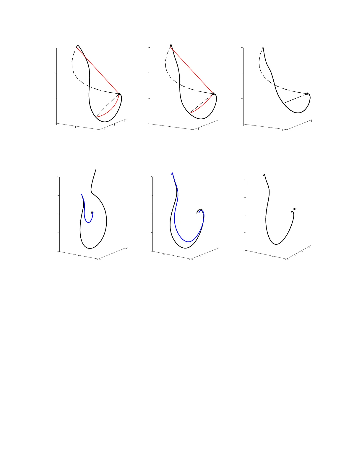
Continuous-time Dynamic Realization f or Nonlinear Stabilization via Contr ol Contraction Metrics Ruigang W ang and Ian R. Manchester Abstract — Nonlinear stabilization using control contraction metric (CCM) method usually in volves an online optimization problem to compute a minimal geodesic (a shortest path) between pair of states, which is not desirable for r eal-time applications. This paper introduces a continuous-time dynamic realization which distrib utes the computational cost of the optimization problem o ver the time domain. The basic idea is to for ce the internal state of the dynamic controller to con verge to a geodesic using covariant derivative information. A numerical example illustrates the proposed approach. I . I N T RO D U C T I O N Stabilization of arbitrary trajectories of nonlinear dy- namical systems is a challenging problem. One solution is to linearize the dynamics around the equilibrium mani- fold and apply the linear parameter-v arying (LPV) control design methods [1]. Howe ver , these approaches generally lack global stability guarantees for the closed-loop nonlinear system. Another approach is to apply nonlinear model pre- dictiv e control (NMPC) [2], which solves an optimal control problem (OCP) in a mo ving horizon way . Due to the comple x dynamic constraints, the computational cost often limits its applications in real-time systems. Contraction theory [3] is an attractiv e tool for the nonlin- ear stabilization problem because it pro vides formal global stability guarantees of the nonlinear system via simple local linear analysis. The underlying idea is to integrate the local stability results along a geodesic (a shortest path w .r .t. certain Riemannian metric) connecting the measured and reference states. Extensions to control design were developed in [4], [5] by introducing the concept of control contraction metric (CCM). Specifically , a CCM is a Riemannian metric for which the Riemannian energy functional of the geodesic between the measured and reference states can be made to decrease exponentially by choosing proper control action. Thus, the CCM can be understood as a differential version of control L yapunov function (CLF). Further e xtensions to distributed control can be found in [6], [7]. Connections and comparisons with LPV based control was discussed in [8]. A static state-feedback realization based on integration along a geodesic was proposed in [4]. Implementation of this controller in volves solving an optimization problem to find a geodesic. This online computation is similar to NMPC, but is of lo wer dimension without dynamic constraints. There exist some indirect methods for geodesic computation, such as phase flo w method [9], fast marching [10] and This work was supported by the Australian Research Council. The authors are with the Australian Centre for Field Robotics, The University of Sydney , Sydney , NSW 2006, Australia (e-mail: ian.manchester@sydney.edu.au ). graph cuts [11]. One drawback of these approaches is the small con ver gence radii. Direct methods construct a finite- dimensional approximation of the online OCP and solve it via nonlinear programming (NLP). T ypical discretization methods include single/multiple shooting [12] and global pseudospectral [13]. Recently , an efficient approach using the Chebyshev pseudospectral was proposed in [14]. Although the computational time is significantly reduced compared with the shooting method, online optimization is still not desirable for time-critical applications. In this paper , we propose a continuous-time dynamic realization approach to address this issue. Inspired by a recent continuous-time MPC scheme [15], [16], the proposed approach makes continuous improvements to the integral path rather than solving a full optimization problem on- line. Specifically , the dynamic controller use forward flows generated by the plant model and gradient information of Riemannian energy functional to force its internal state (a path connecting the reference point to the measured state) to con verge to a geodesic. The control output uses the same integration technique of [4] with integrals computed over the dynamic controller’ s internal state. W e will consider state- feedback realization for both nominal and perturbed systems. It is shown that the nominal closed-loop system is globally exponential stable and the path con ver ges to a geodesic if the controller dynamics are sufficiently fast with respect to the plant dynamics. For the robust case where the system is perturbed by bounded additiv e disturbances, one endpoint of the path would deviate from the measured state, which may lead to closed-loop instability . Robust stability is achie ved by adding state feedback to the path dynamics. The structure of the paper is as follows. Section II giv es some preliminaries results on CCM-based control design. In Section III we detail the proposed continuous-time dynamic realization. A numerical example is presented in Section IV to illustrati ve the effecti veness of this approach. I I . P R E L I M I N A R I E S A. Notation W e use | x | to denote the standard Euclidean norm of a real vector x . The nonnegativ e reals are denoted R + := [0 , ∞ ) . The space L e 2 is the set of vector signals f on R + whose causal truncation to any finite interval [0 , T ] has finite squared norm, i.e. q R T 0 | f ( t ) | 2 dt < ∞ . For symmetric matrices A and B , the notation A ≺ B ( A  B ) means that B − A is positiv e (semi)definite. A Riemannian metric on R n is a symmetric positiv e- definite matrix function M ( x ) , smooth in x , which defines a smooth inner product h δ 1 , δ 2 i := δ > 1 M ( x ) δ 2 for an y two tangent vectors δ 1 , δ 2 at the point x , and the norm k δ k M = p h δ, δ i . A metric is called uniformly bounded if α 1 I  M ( x )  α 2 I , ∀ x , for some constants α 2 ≥ α 1 > 0 . Let Γ( x, y ) be the set of smooth paths joining two points x and y in R n , where each c ∈ Γ( x, y ) is a smooth map c : [0 , 1] → R n and satisfying c (0) = x and c (1) = y . W e use the notation c ( s ) , s ∈ [0 , 1] and c s := ∂ c ∂ s . Given a metric M ( x ) , we can define the Riemannian length and energy functional of c as follo ws L ( c ) := Z 1 0 k c s k M ds, E ( c ) := Z 1 0 k c s k 2 M ds respectiv ely . The Riemannian distance d ( x, y ) between two points is the length of the shortest path between them, i.e., d ( x, y ) := inf c ∈ Γ( x,y ) L ( c ) . Under the conditions of the Hopf-Rinow theorem, there exists a geodesic (minimum- length curve) γ ∈ Γ( x, y ) such that d ( x, y ) = L ( γ ) . Fur- thermore, we ha ve E ( γ ) = L ( γ ) 2 = h γ s , γ s i , ∀ s ∈ [0 , 1] . Let Γ( x, y , t ) be the set of smooth time-varying paths c : R × [0 , 1] → R n connecting smooth signals x ( t ) and y ( t ) . W e also use c ( t ) := c ( t, · ) and ˙ c := dc dt . The formula for first variation of energy [17, p. 195] gives the time deriv ati ve of the energy functional E ( t ) := E ( c ( t )) as follows 1 2 dE dt = h ˙ c, c s i   s =1 s =0 − Z 1 0 h ˙ c, ∇ c s c s i ds (1) where ∇ is the Riemannian connection induced by the metric M ( x ) , and ∇ c s c s is the covariant deri vati ve. A smooth curve c is a geodesic if and only if ∇ c s c s = 0 . B. Contr ol Contraction Metrics Consider nonlinear control-af fine systems of the form ˙ x = F ( x, u ) := f ( x ) + B ( x ) u (2) where x ( t ) ∈ R n and u ( t ) ∈ R m are state and control at time t ∈ R + := [0 , ∞ ) , respectiv ely . For simplicity , f and B are assumed to be smooth and time-inv ariant. W e denote the i th column of B ( x ) by b i ( x ) . For the system (2) we define a refer ence trajectory to be any set of signals x ∗ , u ∗ all in L e 2 and satisfying (2) on R + . A reference trajectory ( x ∗ , u ∗ ) is said to be globally exponentially stabilized by a feedback controller u = κ ( x, x ∗ , u ∗ ) if for any initial state x (0) ∈ R n , a unique closed-loop solution x ( t ) exists for all t ∈ R + and satisfies | x ( t ) − x ∗ ( t ) | ≤ R e − λt | x (0) − x ∗ (0) | (3) where R > 0 is the o vershoot, and λ > 0 the rate. System (2) is said to be universally e xponentially stabilizable if ev ery forward-complete solution ( x ∗ , u ∗ ) is globally exponentially stabilizable. Note that univ ersal stabilizablity is a strong condition than global stabilizablity of a particular solution. Nonlinear stabilization using control contraction metric (CCM) ([4]) is a constructive approach to achiev e univ ersal stability . For the offline design stage, it applies linear system theory to the control synthesis of the local linearized system – differ ential dynamics : ˙ δ x = A ( x, u ) δ x + B ( x ) δ u (4) where A = ∂ f ∂ x + P m i =1 ∂ b i ∂ x u i . Specifically , we construct a differential feedback law: δ u = K ( x ) δ x (5) where K = Y W − 1 with W ( x ) ∈ R n × n and Y ( x ) ∈ R m × n obtained from the following parameter-dependent linear ma- trix inequality (LMI): − ˙ W + AW + W A > − B Y − Y > B > + 2 λW  0 . (6) From the abov e inequality , the controller (5) achieves expo- nential stability for (4): d dt k δ x k 2 M = δ > x ˙ M δ x + 2 δ > x M ( A + B K ) δ x ≤ − 2 λ k δ x k 2 M (7) where M ( x ) = W − 1 ( x ) is called a CCM. A static (memoryless) realization of the controller was proposed in [4], which includes three steps: 1) Compute a minimal geodesic γ ( t ) := argmin c ∈ Γ( x ∗ ( t ) ,x ( t )) E ( c ) . (8) 2) Integrate (5) over γ , i.e., κ γ ( t, s ) := u ∗ ( t ) + Z s 0 K ( γ ( t, s )) γ s ( t, s ) d s . (9) 3) Implement the state-feedback control u = κ ( x, x ∗ , u ∗ ) := κ γ ( t, 1) . (10) This static realization achieves universally e xponential sta- bility with ov ershoot R = q α 2 α 1 and rate λ . If there e xists a smooth coordinate transformation z = h ( x ) satisfying δ > z δ z = δ > x M ( x ) δ x , we can compute the geodesics directly via γ ( s ) = h − 1 ( z ∗ (1 − s ) + z s ) where z ∗ = h ( x ∗ ) and z = h ( x ) . Ho wev er , for general cases, the computation of geodesics in volves an optimization problem (8), which is not desired for time-critical applications. I I I . C O N T I N U O U S - T I M E D Y N A M I C R E A L I Z AT I O N In this section, we introduce a continuous dynamic control realization which keeps Step 2) and 3) unchanged but replace Step 1) with a dynamical system whose internal state is a path joining x ∗ ( t ) to x ( t ) . This path dynamics solves a geodesic computation problem in parallel with the plant system. As shown in Fig. 1, we will consider two scenarios: nominal and robust state feedback. In particular , for the robust case, we assume that the system (2) is perturbed by bounded additi ve disturbances, i.e., ˙ x = F ( x, u ) + d (11) with k d ( t ) k ≤ ∆ for all t ∈ R + . x ∗ x ˙ c c s γ c x ∗ x ˆ x ˙ c c s γ c (a) Nominal case (b) Robust case Fig. 1. Geometric illustrations of the continuous-time dynamic realization: red – path c ( t, · ) , blue – flows c ( · , s ) , dash – geodesic γ ( t ) . A. Nominal State F eedback First, we consider the continuous-time dynamic realization via the forward flow defined by (2): ˙ c = f ( t, s ) := F ( c ( t, s ) , κ c ( t, s )) u = κ c ( t, 1) (12) where the initial state is c (0 , s ) = sx (0) + (1 − s ) x ∗ (0) . Then the endpoint dynamics can be represented by ˙ c ( t, 0) = F ( x ∗ , u ∗ ) , (13a) ˙ c ( t, 1) = f ( x, u ) . (13b) It is easy to v erify that c ( t, 0) = x ∗ ( t ) and c ( t, 1) = x ( t ) for all t ∈ R + since c (0 , 0) = x ∗ (0) and c (0 , 1) = x (0) . Moreov er , integration of (7) over c ( t ) giv es 1 2 ˙ E = h f ( t, s ) , c s i   s =1 s =0 − Z 1 0 h f ( t, s ) , ∇ c s c s i ds ≤ − λE . (14) Globally e xponential stability is achieved but perhaps with larger ov ershoot since c ( t ) generally does not con ver ge to a geodesic γ ( t ) . Now we consider an alternati ve path dynamics: ˙ c = f ( t, s ) + α ( s ) ∇ c s c s (15) where α : [0 , 1] → R + is a smooth weighting function satis- fying α (0) = α (1) = 0 . Here the cov ariant deriv ati ve ∇ c s c s can be taken as the gradient information of the geodesic op- timization problem (8). W e define the normalized weighting function as η ( s ) = α ( s ) /α with α = max s ∈ [0 , 1] α ( s ) . Then, the nominal stability is given as follows. Theorem 1. F or any weighting function α ( s ) , the system (2) subject to the control law (15) is universally exponentially stable. If the parameter α is chosen to be sufficiently larg e, then the contr oller internal state c ( t, · ) con ver ges to a geodesic γ ( t, · ) ∈ Γ( x ∗ , x, t ) before x ( t ) con verg es to x ∗ ( t ) . Pr oof. From (14), we have 1 2 ˙ E ≤ − λE − α Z 1 0 η ( s ) k∇ c s c s k 2 M ds ≤ − λE . (16) Univ ersal stability of the nominal system (2) follows as the length of c ( t ) shrinks exponentially . Choose a constant τ ∈ (0 , 1) , from Lemma 3 we can online adjust the weighting function η such that the follo wing inequality holds: 1 2 ˙ E ≤ − λE − α τ Z 1 0 k∇ c s c s k 2 M ds. (17) W ith a sufficiently lar ge α , the closed-loop system can be decomposed into two time-scale subsystems: slow dynamics (2) and fast dynamics (15). The covariant deriv ativ e ∇ c s c s will be forced to conv erge to 0 (i.e., the path c ( t, · ) con v erges to a geodesic γ ( t, · ) ∈ Γ( x ∗ , x, t ) ) before the con vergence of the state x ( t ) to x ∗ ( t ) . Remark 1 . As shown in Section III-C, the online implemen- tation only computes a finite number of flows c ( t, s j ) , j = 0 , 1 , . . . , N digitally using forward-Euler or Runge-Kutta methods with a sufficiently small sampling time τ s . Thus, α cannot be chosen to be arbitrary large due to numerical stability consideration and the parameters ( s 0 , s 1 ) for the weighting function η ( s ) in (30) cannot be chosen to be arbitrary close to (0 , 1) . Although the path c ( t, · ) may not follow γ ( t, · ) exactly , it can still con ver ge to a small neighborhood of γ ( t, · ) . B. Robust State F eedbac k When system (2) is perturbed by external disturbances, the state trajectory x ( · ) generally does not coincide with the endpoint trajectory c ( · , 1) generated by the path dynamics (15). Let ˆ x ( t ) = c ( t, 1) and ˜ x ( t ) = x ( t ) − ˆ x ( t ) . T o reduce the disturbance effect on ˜ x , we use the following path dynamics ˙ c = f ( t, s ) + α ( s ) ∇ c s c s + β ( s ) ˜ x ( t ) (18) where β ( s ) = β ζ ( s ) with ζ : [0 , 1] → [0 , 1] as a nondecreas- ing function satisfying ζ (0) = 0 and ζ (1) = 1 . Note that, for the nominal case, the abov e system is equiv alent to the path dynamics (15). If the disturbance bound ∆ is suf ficiently small, the dynamics of ˜ x ( · ) can be approximated by ˙ ˜ x = ( A cl ( ˆ x, ˆ u ) − β I ) ˜ x + d (19) where A cl ( ˆ x, ˆ u ) = A ( ˆ x, ˆ u ) + B ( ˆ x ) K ( ˆ x ) with ˆ u = κ c ( t, 1) . From (7) we hav e that the maximum eigen v alue of A cl ( ˆ x, ˆ u ) is no lar ger than − λ . Therefore, the error bound for ˜ x is | ˜ x ( t ) | ≤ ∆ β + λ , ∀ t ∈ R + . (20) The time deri vati ve of the energy functional satisfies 1 2 ˙ E ≤ − λE +  β ˜ x, c s ( t, 1)  − Z 1 0  β ˜ x, ζ ∇ c s c s  ds − ατ Z 1 0 k∇ c s c s k M ds ≤ − λE +  β ˜ x, c s ( t, 1)  +  2 4 k β ˜ x k 2 M − ατ 2 Z 1 0 k∇ c s c s k M ds (21) Im z Re z x ( t ) x ∗ ( t ) Fig. 2. Illustration of discretization of path c ( t ) using Chebyshev polynomials. where  ≥ p 2 /ατ . The closed-loop robust stability is giv en as follo ws. Theorem 2. Consider the perturbed system (11) and the continuous-time dynamic contr ol r ealization (18) . If the parameter α, β are sufficiently larg e, the closed-loop system is r ob ust stable with r espect to the set Ω( x ∗ ) = { x ∈ R n : | x − x ∗ | ≤ R ∆ /λ } (22) wher e R = (1+ √ 1+ λ 2 ) β 2( β + λ ) R + λ β + λ . Pr oof. If α is sufficiently large, we can conclude from (21) that c ( t ) con verges to γ ( t ) for t ≥ T where T is sufficiently large. This leads to 1 2 ˙ E ≤ − λE +  β ˜ x, γ s ( t, 1)  +  4 k β ˜ x k 2 M . (23) W ith the facts that E ( γ ) = h γ s , γ s i , ∀ s ∈ [0 , 1] and | ˜ x | ≤ ∆ β + λ , there exists a T 0 > T such that the following inequality holds for t ≥ T 0 : | ˆ x ( t ) − x ∗ ( t ) | ≤ (1 + √ 1 + λ 2 ) β 2( β + λ ) R ∆ (24) which leads to | x ( t ) − x ∗ ( t ) | ≤ | ˆ x ( t ) − x ∗ ( t ) | + | ˜ x | ≤ R ∆ /λ. (25) Remark 2 . The parameter α represents the con v ergence speed of c ( t ) to a geodesic γ ( t ) connecting x ∗ ( t ) to ˆ x ( t ) while the parameter β controls the con vergence speed of ˆ x ( t ) to x ( t ) . The parameter  af fects the size of in v ariant set. When α, β → ∞ and  → 0 , we ha ve R → R which implies that dynamic realization achie ves the same inv ariant set as the geodesic based static realization (10). C. Implementation The path dynamics is an infinite-dimensional system as its internal state c ( t ) is a smooth function over [0 , 1] . For online implementation, we approximate c ( t ) with Chebyshev polynomial expansion at time t . This is a finite-dimensional approximation based on the samples of the path at Chebyshev nodes. In this way , the path dynamics is discretized into a finite set of dynamical systems whose state dimension is same as the original nonlinear plant. Those systems are solved in parallel with the nonlinear plant and the solutions are used to construct an approximate path at the next time step. As time in volv es, this path con verges to a geodesic due to the forward and gradient descent flows. This approach is different from [14] which uses Chebyshev polynomials to discretize the geodesic computation problem (8) at each time point. A finite-dimensional NLP is iterativ ely solv ed online, and the optimal solution is then used to construct a geodesic. Thus, the online computation time of the proposed approach is expected to be much smaller, compared with the optimization based approach [14]. Firstly , we recall some standard results of approximation theory using Chebyshev polynomials (see [18] for details). The first-kind Chebyshe v polynomials T k ( x ) ov er the inter- val [ − 1 , 1] are defined recursiv ely by T k +1 ( x ) = 2 xT k ( x ) − T k − 1 ( x ) , k = 1 , 2 , 3 , . . . (26) with starting values T 0 ( x ) = 1 and T 1 ( x ) = x . Under the coordinate transform x = cos( θ ) , θ ∈ [0 , π ] , we have T k (cos θ ) = cos( k θ ) . A continuous function f ( x ) ov er the interval [ − 1 , 1] can be approximated by ˜ f (cos θ ) = a 0 2 + N X k =1 a k cos( k θ ) (27) where the coefficients { a k } 0 ≤ k ≤ N can be obtained by ap- ply discrete cosine transform to the samples of f at the Chebyshev nodes x j = cos( j π / N ) , j = 0 , 1 , . . . , N . Other operations on f such as integration and differentiation can also be efficiently approximated by Chebyshev polynomials. Since the CCM-based control design is in variant under coordinate transformations [4], we can reparameterize the path c ( t, · ) from [0 , 1] to [ − 1 , 1] . For the online implemen- tation of dynamic controllers (12), (15) and (22), instead of computing the infinite-dimensional state c ( t, · ) , we only compute the flo ws at s j = cos( j π / N ) , j = 0 , 1 , . . . , N , as shown in Fig. 2. Base on the values of c ( t, s j ) , the state c ( t, · ) is reconstructed as c ( t, s ) = c ( t ) T ( s ) where c ( t ) ∈ R n × ( N +1) and T ( s ) = [ T 0 ( s ) , T 1 ( s ) , . . . , T N ( s )] > . W ith this, we can compute smooth representations of the deri vati ve ∂ c ∂ s , covariant deriv ativ e ∇ c s c s , differential control δ u and its integration κ c . By taking samples of these functions at the Chebyshev nodes, we can obtain the right hand side of the dynamic controllers (12), (15) and (22). Remark 3 . Note that the abov e computation only in volv es a series of simple online operations such as additions, multipli- cations, differentiation and inte gration o ver a smooth func- tion c ( t, · ) . Due to the absence of complex operations (e.g. solutions of optimization problems) the online computational time can be estimated a priori . This information can be used to choose a sufficiently small sampling time τ s such that the flows c ( · , s j ) , j = 0 , 1 , . . . , N can be computed digitally by using forward-Euler or Runge-Kutta approximation methods. 0 1 2 3 4 5 -6 -4 -2 0 2 4 6 Forward Gradient Geodesic 0 0.1 0.2 5.4 5.6 5.8 Fig. 3. Exponential decay rate of the Riemannian energy of integral paths. I V . I L L U S T R A T I V E E X A M P L E W e consider the follo wing nonlinear system   ˙ x 1 ˙ x 2 ˙ x 3   =   − x 1 + x 3 x 2 1 − x 2 − 2 x 1 x 2 + x 3 − x 2   +   0 0 1   u. (28) This system is not feedback linearizable and highly unstable. The control synthesis problem (6) w as solved by SOS programming with LMI toolbox - Y almip [19]. A control contraction metric with λ = 1 was found to be W ( x ) = W 0 + W 1 x 1 + W 2 x 2 1 where W 0 =   2 . 686 0 . 237 − 1 . 816 0 . 237 16 . 265 2 . 006 − 1 . 816 2 . 006 6 . 395   W 1 =   0 − 5 . 373 0 − 5 . 373 − 0 . 948 3 . 631 0 3 . 631 0   , W 2 =   0 0 0 0 10 . 747 0 0 0 0   and Y ( x ) = − 1 2 ρ ( x ) B > with ρ ( x ) = 19 . 614 + 1 . 386 x 1 + 9 . 616 x 2 1 . From [4, Lemma 1], this metric is complete and thus a minimal geodesic exists for e very pair of points. For online implementation, we use Chebyshev basis functions with maximal order N = 4 to reconstruct the path c ( t, · ) . The toolbox for Chebyshev polynomials manipulation is called chebfun [20], which is an open source software. For the nominal case, we compare the results of three different realizations: forward flow based dynamic con- troller (12), gradient flow based dynamic controller (15) and geodesic based static controller (10). The initial condition and setpoint are chosen as x (0) = [9 , 9 , 9] > and x ∗ = [0 , 0 , 0] > , respecti vely . From Fig. 3, the Riemannian energy functional of the inte gral path c decays exponentially with rate of 2 λ for these three controllers. The proposed approach con ver ges to a geodesic within time of 0 . 05 by feeding the cov ariant deriv ati ve to the path dynamics. W ithout this term, the path in forward flow based approach does not con ver ge to a geodesic, which leads to a larger overshoot estimation for exponential stability . Fig. 4 depicts the time e volution of inte gral paths c ( t, · ) and geodesics γ ( t ) for different controllers. Compared with the forward flow approach, giv en the same initial condition (a straight line), the state c ( t, · ) of the proposed approach conv erges to the neighborhood of a geodesic γ ( t ) . For the robust case where the dynamics of x 1 is perturbed by a persistent external disturbance d ( t ) = 2 , we test those three controllers using the same initial state and setpoint. Fig. 5 shows that the forward flow approach is unstable due to the lack of feedback, although the state prediction ˆ x ( t ) con ver ges to the setpoint. For the proposed approach, the state prediction ˆ x ( t ) remains in a neighborhood of x ( t ) due to the feedback term in (22). And the closed-loop system has a similar response compared to the geodesic based approach. V . C O N C L U S I O N In this paper we proposed a continuous-time dynamic realization for control contraction metrics based nonlinear stabilization. It distributes the online geodesic computation across the time domain. Both universal stability for the nom- inal system and robust stability for the perturbed system are guaranteed. Simulation results demonstrated the ef fectiv eness of the proposed approach. A P P E N D I X Lemma 3. F or any c ∈ Γ( x ∗ , x ) and any τ ∈ (0 , 1) , there exists a weighting function η : [0 , 1] → [0 , 1] such that Z 1 0 η ( s ) k∇ c s c s k 2 M ds ≥ τ Z 1 0 k∇ c s c s k 2 M ds. (29) Pr oof. W e define µ c ( s ) := R s 0 k∇ c s c s k 2 M d s . Since M ( x ) is a uniformly bounded metric and c is a smooth curve, the cov ariant deriv ati ve ∇ c s c s is smooth and bounded for any s ∈ [0 , 1] . Thus, µ c is a nondecreasing function with µ c (0) = 0 and µ c (1) = C < ∞ . If c is a geodesic (i.e., C = 0 ), the weighting function η ( s ) = 0 satisfies (29). Otherwise, for any τ ∈ (0 , 1) , we can find s 0 = arg inf µ − 1 c ((1 − τ ) C / 2) and s 1 = arg sup µ − 1 c ((1 + τ ) C / 2) . It is easy to check that 0 < s 0 < s 1 < 1 and µ c ( s 1 ) − µ c ( s 0 ) ≥ τ C since µ c is nondecreasing. Now we choose the weighting function to be η ( s ) = π s 0 0 ( s )  1 − π 1 s 1 ( s )  (30) where π b a : R → [0 , 1] is a smooth and nondecreasing such that π b a ( s ) = 0 , ∀ s ≤ a and π b a ( s ) = 1 , ∀ s ≥ b . This weighting function satisfies (29) as Z 1 0 η ( s ) k∇ c s c s k 2 M ds ≥ Z s 1 s 0 k∇ c s c s k 2 M ds ≥ τ C. R E F E R E N C E S [1] W . J. Rugh and J. S. Shamma, “Research on gain scheduling, ” Automatica , vol. 36, pp. 1401–1425, 2000. [2] F . Allg ¨ ower and A. Zheng, Nonlinear model predictive contr ol . Birkh ¨ auser , 2012, vol. 26. [3] W . Lohmiller and J.-J. E. Slotine, “On contraction analysis for non- linear systems, ” Automatica , vol. 34, pp. 683–696, 1998. x(0) 0 x * Forward flow -5 10 0 10 5 10 5 20 0 x(0) 0 x * Gradient flow -5 10 10 0 5 10 5 20 0 x(0) 0 x * Geodesic flow 10 -5 10 0 5 10 5 20 0 Fig. 4. Nominal state-feedback control: red – path c ( t, · ) at two time points, black dash – geodesic γ ( t, · ) , black solid – state trajectory x ( t ) . x(5) -50 x(0) -20 Forward flow x* -10 0 10 20 20 0 0 50 -20 x(0) x* -10 0 Gradient flow -5 0 5 10 10 10 5 20 0 30 -5 x(0) x* 0 -10 Geodesic flow -5 0 10 10 5 10 5 20 0 30 -5 Fig. 5. Robust state-feedback control: blue – predicted state trajectory c ( t, 1) , black solid – state trajectory x ( t ) . [4] I. R. Manchester and J.-J. E. Slotine, “Control contraction metrics: Con vex and intrinsic criteria for nonlinear feedback design, ” IEEE T rans. Autom. Control , vol. 62, no. 6, pp. 3046–3053, Jun. 2017. [5] ——, “Robust control contraction metrics: A con vex approach to nonlinear state-feedback H ∞ control, ” IEEE Control Syst. Lett. , vol. 2, no. 3, pp. 333–338, Jul. 2018. [6] R. W ang, I. R. Manchester, and J. Bao, “Distributed economic MPC with separable control contraction metrics, ” IEEE Contr ol Syst. Lett. , vol. 1, pp. 104–109, 2017. [7] H. S. Shiromoto, M. Re vay , and I. R. Manchester , “Distributed nonlinear control design using separable control contraction metrics, ” IEEE T rans. Control Netw . Syst. , 2018. [8] R. W ang, R. T ´ oth, and I. R. Manchester , “ A comparison of LPV gain scheduling and control contraction metrics for nonlinear control, ” accepted by IF A C W orkshop on Linear Parameter-V arying Systems, 2019. [9] L. Y ing and E. J. Candes, “Fast geodesics computation with the phase flow method, ” J. Comput. Phys. , vol. 220, no. 1, pp. 6–18, 2006. [10] R. Kimmel and J. A. Sethian, “Computing geodesic paths on mani- folds, ” Pr oc. National Academy of Sciences , vol. 95, no. 15, pp. 8431– 8435, 1998. [11] Y . Boyko v and V . Kolmogorov , “Computing geodesics and minimal surfaces via graph cuts, ” in Proc. IEEE Int. Conf. Comput. V ision , 2003, pp. 26–33. [12] B. Houska, H. J. Ferreau, and M. Diehl, “ An auto-generated real- time iteration algorithm for nonlinear MPC in the microsecond range, ” Automatica , vol. 47, no. 10, pp. 2279–2285, 2011. [13] D. Garg, M. Patterson, W . W . Hager , A. V . Rao, D. A. Benson, and G. T . Huntington, “ A unified framework for the numerical solution of optimal control problems using pseudospectral methods, ” Automatica , vol. 46, no. 11, pp. 1843–1851, 2010. [14] K. Leung and I. R. Manchester, “Nonlinear stabilization via con- trol contraction metrics: A pseudospectral approach for computing geodesics, ” in Pr oc. Amer . Contr ol Conf. (ACC), Seattle, W A , 2017, pp. 1284–1289. [15] C. Feller and C. Ebenbauer, “Continuous-time linear MPC algorithms based on relaxed logarithmic barrier functions, ” IF A C Proc. V ol. , vol. 47, no. 3, pp. 2481–2488, 2014. [16] M. M. Nicotra, D. Liao-McPherson, and I. V . Kolmano vsky , “Em- bedding constrained model predictiv e control in a continuous-time dynamic feedback, ” IEEE T rans. Autom. Control , vol. 64, no. 5, pp. 1932–1946, 2018. [17] M. P . Do Carmo, Riemannian geometry . Boston, MA: Springer, 1992. [18] L. N. Trefethen, Appr oximation Theory and Approximation Practice . Philadelphia, P A: SIAM, 2013. [19] J. Lofberg, “Y ALMIP: A toolbox for modeling and optimization in MA TLAB, ” in Proc. CACSD conf., New Orleans, LA, USA , 2004, pp. 284–289. [20] T . A. Driscoll, N. Hale, and L. N. Trefethen, Chebfun Guide . P afnuty Publications, 2014.