Stochastic Geometry of Network of Randomly Distributed Moving Vehicles on a Highway

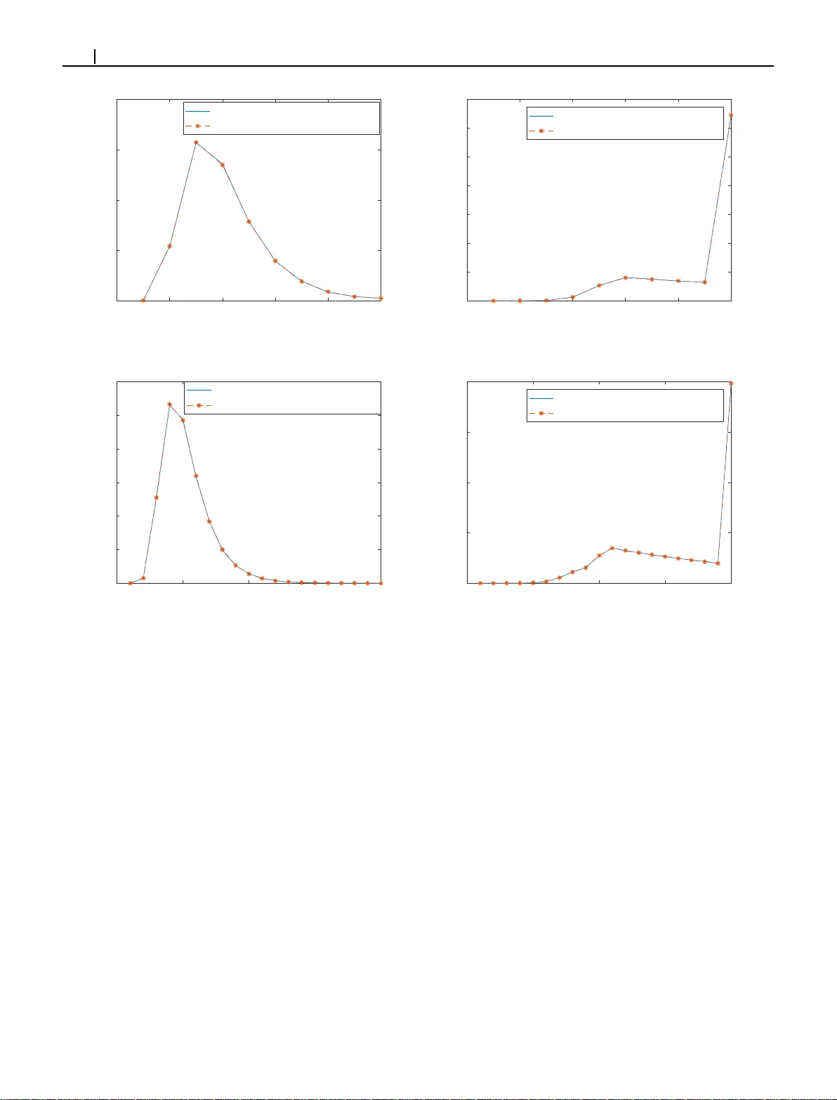
Received: Added at production Revised: Added at production Accepted: Added at production DOI: xxx/xxxx ARTICLE TYPE Stoc hastic G eometry of Netw ork of Randoml y Distri buted Mo vi ng V ehicles on a Highw a y Gleb Dubosarskii | Ser guei Prim ak | Xianbin W ang Corr espondence Gleb Dubosarskii, Department of Electrical and Computer E nginee ring, W estern Univ ersit y , Ontario, Canada. Email: gdubosar@uw o.ca Summary V ehicular ad-hoc ne tworks (V ANET s) hav e become an extensivel y studied top ic in contempo rar y research. One of the fundamen tal pro blems that has ar isen in such research is un derstandin g t he network statistical prop er ties, such a s the clu ster n u m- ber dis tr ibution an d t he clust er size d istribu tio n. In this p aper, we an alyze these character istics in t he case in which vehicles are located on a straight road. Assum- ing t he Rayleigh fading model and a p robabilistic model o f inter vehicle distan c e , we der ive prob abilistic distr ibutions of th e aforementioned con nectivity char a cter istics, as well as distributio ns of the biggest clu ster and t he nu mber of disco nnected vehi- cles. All o f t he re sults are con fir m ed by simulations car r ied o ut f or the realistic values of p a rameters. KEYW ORDS: v ehicle netw ork, clustering, net work evol ution 1 INTRODUCTION V ehicular ad-h oc netw orks (V ANET s) are de veloped to provide intelligent transpor tation th at improv es road safe ty , reduces transpor tation time, and decreases road co n gesti on. One of t he possible signal p ropagation scenar ios is vehicle-to-vehicle (V2V) communication, which means a direct connection betw een two nearby v ehicles. Another considered scenario is vehicle-to- infrastructur e (V2 I) communication, in which a vehicle sends and receives a signal from Road Side Units (RSUs) at t he side of the road. RSUs f or m infrastructu re th at improv es th e per formance of V ANET s an d enhances inf or mation distribu tion . Multihop information propagation in V ANET is limited by high vehicular speed and frequent disconnections. To address these issues, significant progress was made in routing protocols 1,2,3,4,5 dev eloped to reduce latency an d stabilize the connection betw een vehicles, allowing vehicles to receive r eal- time tra vel-related information. The high mobility of vehicles an d th e changing netw ork topology lead to difficulties in t he distr ibution of con tent, including images and video. To m itigate t hese sho r tco mings, cloud architectures are proposed that allo w f or t he sharing of abundant resources, and for the regulating of netw ork connectivity specifications. In 6 , th e scheme, in which parked vehicles can play the role of RSUs, is p ropo sed. In 7 , RSU clo u d is introduced that has t he ab ility to dynamically reconfigur e data forwarding r ules in t he netw ork to meet frequently changing ser vice demands. Ar ticle 8 integrates both RSU and vehicles into one comput ational netw ork that provides services, and p roposes an optimal strategy for resour ce allocation. V ANET is a highly dy namic n etw ork, m aking it difficult to anal yze from a d eterministic point of view . This is the reason th at statis tical meth ods are used to make predictions under the assumption of par ticular probabilistic d istributions of vehicles on t he road and models of signal tran smission. Consider ing th is problem on a real map seems to be an impo ssible task, so, in most 2 Gleb Dubosarskii E T AL ar ticles, the auth o rs limit themselv es to the cases of a highwa y or a crossroad. Ar ticles 9,10,11,12,13 are devo ted to th e inv estig ation of statis tical characteristics of the networ k, such as t he number of clusters, cluster size, and t he number of disconnected vehicles. Let us discuss the con ten t of t hese ar ticles in more detail. I n 9 , it is assumed that the probabilistic distribution of distance between cars is known, and as soon as t he distance between neig hbor ing vehicles does not ex ceed transmission range 𝐿 , they are alw ay s able to establish a con n ection. Under these assumptions, probab ility distribution of information propagation d istance is f ound, as w ell as its expected value and variation. Ar ticles 10,13 discuss more realistic commun ication channel models, such as Raylei gh, Rician, an d W eibu ll fading channels. For each of th ese m odels, the probability of connection betw een neighbor in g vehicles and the probability of full connectivity of the networ k are der ived. Th e auth ors of 11 consider a mo re co m plex case in which the cars are located betw een tw o RSUs, but use a simple th e mod el of the commu nication channel: th ey assume (as in 9 ) t hat the vehicles are alwa ys connected within the constant transmission ran ge and disconn ected other wise. Such ad vanced n etw ork character istics as expected n umber of clusters, netw ork connectivity probability , e xpected number o f vehicles required for a V ANET to be fully co n nected, and expected n etw ork capacity are f ound wit h in t he fr am ew o rk of t his mod el. In 12 , t he aut hors suggest that vehicles in t he cluster do not communicate with each other, but, instead, all vehicles communicate with th e main car . U nder presumption of the Ra yleigh fading channel mod el, t he Marko v model of packet transmission, an d the PHY deco ding failure model, t h e a verage packet loss probability is der ived. In 14,15,16 , t he evolution o f the netw ork over time is considered. In 14 , a case in which a signal is transmitted to vehicles moving in the opposite direction an d then sent back to th e initial side is in ves tigated. The probability of such a successful two-hop connection is der ived und er the assumption that vehicles move at a constant speed. Article 15 f ocuses on t he study of link duration in t he specific case, in which the speed of the vehicles g row s linearl y , reaches the limit, and then remains constant. In ou r article 16 , the netw ork ev olution is inv estig ated und er the presumption that the connection betw een consecutive cars is preserved accord in g to the Marko v probabilis tic model; its p ar ameters are explicitl y e xpressed through t he netw ork macro parameters. Under th ese co nditions, explicit formu las are obt ain ed for t he probab ility d istribution of link duration b etw een con sequent vehicles, t he cluster exis tence, and other fun d amental networ k character istics. In t h is ar ticle, w e consider t he case of a vehicle netw ork on a hig h wa y . Our goal is to g ive an extended descr iption o f th e netw ork, n ot only in term s o f av erage values an d variance, as is don e in the p revious ar ticles (such as 11 ), but to find the whole distribution o f the n u mber of clusters, cluster size, and t he numb er of disconnected vehicles (here we call t hem idle vehicles ). W e u se a more realistic mod el of the commu nication channel (Ray leigh fading channel) than in 9,11 . W e advance fur ther t han the author s of 10,12,13 and find the distribution of t he num b er of clusters and cluster size. T h e difference betw een t his ar ticle and 14,15,16 is that we d o not consider the ev olution of the netw ork ov er time, but concentrate in detail on more nuanced connectivity characteristics at a fix ed mo ment in time. Moreov er, to the best of our kn ow ledge, w e are the first to inv estigat e the d istribution of the b iggest cluster size. W e assume that e very car co m municates o nly with the nearest car, in front, an d behind it. This assumption is m ad e in t he previous statistical research in t his area, in order to make the mod el simple enoug h to analyze. Under the presumption of Ray leigh fading model and known density fun ction of inter vehicle distance, we express t he abov e mentioned distributions in term s of kn own parameters of the network. Our model can be applied to other scenar ios if the probab ility of connection between ev ery pair of co nsecutive vehicles has t he same value 𝑝 . W e der ive sev eral interesting results describ in g netw ork connectivity , n am el y , th at t he av erage size of cluster is a constant, approximatel y equaling 1∕ (1 − 𝑝 ) ; the a verage number of clusters is propo r tional to the number of vehicles 𝑛 equaling 1 + ( 𝑛 − 1)(1 − 𝑝 ) ; and in the netw ork, on av erage there is a constant fraction ≈ 1∕(1 − 𝑝 ) 2 of t he idle vehicles. The av erage largest cluster of the netw ork, how e ver , is not a constant and grow s as log 1∕ 𝑝 𝑛 . W e con firm these and oth er theoretical results by simulations car r ied out in th e cases of different car densities and number of car s. The a verages and var iances of t he studied proper ties are sum m ar ized in th e f ollowing table (where 𝛾 = 0 . 577 … is an Euler co nstant): Property A verage V ar iance Number of clu sters 1 + ( 𝑛 − 1)(1 − 𝑝 ) ( 𝑛 − 1 ) 𝑝 (1 − 𝑝 ) Size of clusters (1 − 𝑝 𝑛 )∕(1 − 𝑝 ) (2 𝑝 𝑛 +1 𝑛 − 2 𝑝 𝑛 𝑛 − 𝑝 2 𝑛 − 𝑝 𝑛 +1 + 𝑝 𝑛 + 𝑝 )∕(1 − 𝑝 ) 2 Size of th e biggest cluster ≈ log 1∕ 𝑝 {( 𝑛 − 1 )(1 − 𝑝 )} + 𝛾 ∕ ln(1∕ 𝑝 ) + 0 . 5 ≈ 𝜋 2 ∕ ln 2 (1∕ 𝑝 ) + 1 12 Number of id le cars 2(1 − 𝑝 ) + ( 𝑛 − 2)(1 − 𝑝 ) 2 −3 𝑛𝑝 4 + 10 𝑛𝑝 3 − 11 𝑛𝑝 2 + 4 𝑛𝑝 + 8 𝑝 4 − 22 𝑝 3 + 18 𝑝 2 − 4 𝑝 The studied statis tical characteristics h a ve sev eral practical app lications. C luster size distribution and max imu m cluster size distribution provide us with tools for network load prediction. Also, t his statis tical inf or mation can be used f or secur ity pu r p oses. The cluster size estimation, for e xample, allow s for the prediction of t he number of inf ected v ehicles in the ev ent o f an att ack on a cluster . Estimation of the number of disconnected vehicles makes it possible to ev aluate th e quality of connection, in o rder to make the percentage of disconnected vehicles acceptab l y low . Gleb Dubosarskii E T A L 3 The p aper is organized as follo w s. In section 2 we describe the con nectivity model and der ive a f or mula for th e probability of connection between tw o co nsecutive cars. In 3 we der ive all th e probabilistic distribu tions mentioned abov e. Finall y , in section 4 t he simulation results are p resented and compared to t he calculations don e by the f or mulas f rom section 3. The appen dix is dev oted to a quic k introduction to t h e t heor y of generating functions n eed ed in section 3. W e use the follo wing abb reviations: W e use t he follo wing abb reviations for the connectivity character istics of the netw ork: ClustN um number of clusters in the netw ork ClustSize size of th e cluster BiggestClus t size of th e biggest cluster IdleCars number of disconnected vehicles The follo wing variables and fu nctions are used: 𝑝 probability of connection b etw een two con secutiv e vehicles 𝐺 𝑇 transmit anten n a gain 𝐺 𝑅 receive antenna gain 𝑃 𝑡𝑥 transmit power 𝛼 path loss exponent 𝐾 constant associated with the path loss m o del 𝑑 distance between cars 𝐶 speed of light 𝑊 ther mal noise pow er 𝑘 Boltzmann constant, 𝑘 = 1 . 38 × 10 −23 𝐽 ∕ 𝐾 𝑓 𝑐 car r ier frequency 𝑇 0 room temperature 𝐵 transmission ban d width 𝑓 𝛾 ( 𝑥 ) Signal-to-noise ratio probability density function 𝑓 𝑑 ( 𝑥 ) inter vehicle d istance probability d ensity function  𝑘 𝑠  binomial coefficient 𝑐 𝑜𝑒𝑓 𝑓 𝑥 𝑛 𝑓 ( 𝑥 ) coefficient o f t he ter m 𝑥 𝑛 in ser ies 𝑓 ( 𝑥 ) 𝑐 𝑙𝑢𝑠𝑡 ( 𝑁 ) number of clusters of vehicle netw ork 𝑁 𝑐 𝑜𝑢𝑛𝑡 ( 𝑟 ; 𝑁 ) number of clusters of vehicle netw ork 𝑁 ha ving size 𝑟 𝑁 𝑢𝑚 ( 𝑠, 𝑘 ) number of netw orks having 𝑘 clu sters, under condition t hat 𝑠 of t hem h a ve size 𝑟 . 𝛾 Euler constant, 𝛾 = 0 . 577 … 2 NE TW ORK MODEL W e consider the netw ork of randomly distributed car s o n a hig h wa y and suppose that ev er y v ehicle of the networ k can establish a conn ection only with t he closest front and back neighbou rs. W e denote by 𝑑 t he d istance betw een two consecutive vehicles. W e assume that t h e distance betw een vehicles has rando m distribution with density f unction 𝑓 𝑑 ( 𝑥 ) . T ypically it is assumed that d istance betw een cars has e xponential dist r ibution, nor mal distribu tion, gamma distribution o r log-nor mal distribution. These d istributions cor respond to different flow cond itions. For instance, exponential distribution cor respond s to low traffic flow conditions, while high traffic flow conditions are descr ibed b y n or mal distrib u tion. Let us suppose t hat t here are 𝑛 cars on a road and distribution of distance between cars has a mean value 𝑀 , therefore, the a verag e distance b etw een the first and the last car is ( 𝑛 − 1 ) 𝑀 , con sequently , despite the fact t hat the road is long, it is improbable that t he distance between first and last vehicle is very large. W e assume t hat the a verage channel Signal-to-noise ratio (SNR) betw een two consecutive vehicles 𝛾 is calculated using the f ollowing f or mula from 13 : 𝛾 = 𝑃 𝑡𝑥 𝐾 𝑑 𝛼 𝑊 , (1) where 𝑃 𝑡𝑥 is the transmit pow er, 𝛼 is t he path loss exponent and 𝐾 is a co n stant associated with the pat h loss mod el. The parameter 𝐾 is given by the formula 𝐾 = 𝐺 𝑇 𝐺 𝑅 𝐶 2 (4 𝜋 𝑓 𝑐 ) 2 , (2) 4 Gleb Dubosarskii E T AL where 𝐺 𝑇 and 𝐺 𝑅 are the transmit and r eceive antenna gains, 𝐶 is the speed of ligh t and 𝑓 𝑐 is the car r ier frequency . W e assume that t he antenn as are omni direction al 𝐺 𝑇 = 𝐺 𝑅 = 1 (3) and 𝑓 𝑐 = 5 . 9 𝐺 𝐻 𝑧 . The ther mal no ise pow er can be deter m ined by the f or mula 𝑊 = 𝑘𝑇 0 𝐵 , (4) where 𝑘 = 1 . 38 × 1 0 −23 𝐽 ∕ 𝐾 is th e Boltzmann constant, 𝑇 0 ( 𝑇 0 = 300 ◦ 𝐾 ) is t he room temperature, and 𝐵 ( 𝐵 = 10 MHz) is t he transmission ban d width. The SNR density function 𝑓 𝛾 ( 𝑥 ) (is different from 𝑓 𝑑 ) is given by the f or mula 𝑓 𝛾 ( 𝑥 ) = 1 𝛾 𝑒 − 𝑥 ∕ 𝛾 . (5) It is assumed that t here is a co n nection between consecutive cars if 𝛾 is g r eater than the threshold Ψ . Therefore, 𝑃 ( 𝛾 > Ψ) = ∞ ∫ Ψ 𝑓 𝛾 ( 𝑥 ) 𝑑 𝑥 = 𝑒 −Ψ∕ 𝛾 . (6) Let us denote th e probability t hat two consecutive vehicles can establish a connection by 𝑝 . B y using (1), (6) and f ollowi ng the lo g ic of 11 w e can d er ive formu la expressing value of th e probability 𝑝 t h rough inter vehicle density fu nction 𝑓 𝑑 ( 𝑥 ) : 𝑝 = ∞ ∫ 0 𝑃 ( 𝛾 ( 𝑥 ) > Ψ) 𝑓 𝑑 ( 𝑥 ) 𝑑 𝑥 = ∞ ∫ 0 𝑒 − Ψ 𝑥 𝛼 𝑊 𝑃 𝑡𝑥 𝐾 𝑓 𝑑 ( 𝑥 ) 𝑑 𝑥. (7) The value of the parameter 𝑝 lies within an inter val (0 , 1) and plays a prominent role in t he fur ther in ves tigations. It d etermines the quality o f com m unication. A larger value of parameter 𝑝 leads to a better quality of connection an d con sequentl y a b igger size of clusters. 3 CONNECTIVITY OF THE NETW ORK 3.1 Distribution of number of clusters The main achie vement of this ar ticle is t hat we dr ive not only the a verage val ues of various connectivity character istics, as in the p revious ar ticles (see t he Introduction), bu t also their probability distributions and variations. In th is section we inv estig ate such a significant character istic o f th e netw ork as distr ibution of n umber of clusters. I n this section we establish th e f ollowing f or mula f or the probability of number o f clusters 𝐶 𝑙𝑢𝑠𝑡𝑁 𝑢𝑚 equaling 𝑟 : 𝑃 ( 𝐶 𝑙 𝑢𝑠𝑡𝑁 𝑢𝑚 = 𝑟 ) =  𝑛 − 1 𝑟 − 1  𝑝 𝑛 − 𝑟 (1 − 𝑝 ) 𝑟 −1 , (8) where parameter 𝑝 is determined in (7). In oth er words, number o f clusters has bino mial distribution . T o prov e formula (8) we need to better und er stand the str ucture o f the netw ork. The idea behind th e der ivation is to con sider connections b etw een vehicles as Ber no ulli tr ials. There are 𝑛 vehicles in the networ k establishing no more th an 𝑛 − 1 connections betw een each other, thu s, we can think abo ut them as 𝑛 − 1 indepen dent tr ials, in which each of th em is successful if consecutive vehicles can con nect, and u nsuccessful other wise. Clusters are assumed to be formed by a ser ies of se veral consecutive vehicles, therefore, if there are 𝑟 clusters in th e network, th en ex actl y 𝑟 − 1 v ehicles cannot establish a connection. From the abov e we could conclude t hat th e probability 𝑃 ( 𝐶 𝑙𝑢𝑠𝑡𝑁 𝑢𝑚 = 𝑟 ) equals th e probability that in 𝑛 − 1 tr ials exactl y 𝑟 − 1 are unsuccessful with the probability of success 𝑝 . This probability is given by well-known f or mula f or binomial d istribution, which in our case is exactl y formula (8). By using known formulas for mean and variance of binom ial distribution one can der ive that the a verage n umber o f clusters and t heir variance are given by t h e formulas E [ 𝐶 𝑙 𝑢𝑠𝑡𝑁 𝑢𝑚 ] = 1 + ( 𝑛 − 1)(1 − 𝑝 ) , (9) V a r [ 𝐶 𝑙 𝑢𝑠𝑡𝑁 𝑢𝑚 ] = ( 𝑛 − 1) 𝑝 (1 − 𝑝 ) . (10) Gleb Dubosarskii E T A L 5 Here we consider a disconn ected vehicle as a separate cluster . The av erage number o f clusters f or med by at least two cars can be calculated by substracting from (9 ) the a verage nu mber of idle cars der ived later in section 3. 4 (see t he formu la (40)). Therefore, it is given by the follo wing formula: 1 + ( 𝑛 − 1)(1 − 𝑝 ) − 2( 1 − 𝑝 ) − ( 𝑛 − 2)(1 − 𝑝 ) 2 . (11) Remar k. W e see from (9) that the av erage number o f clusters in t he sys tem grow s linearly with t he num b er of vehicles with a growth factor 1 − 𝑝 . 3.2 Distribution of cluster size In t his subsection we concen trate on findin g p robab ility 𝑃 ( 𝐶 𝑙 𝑢𝑠𝑡𝑆 𝑖𝑧𝑒 = 𝑟 ) t hat size of arbitrar y cluster in th e n etw ork is 𝑟 . W e prov e the follo wing f or mula: 𝑃 ( 𝐶 𝑙 𝑢𝑠𝑡𝑆 𝑖𝑧𝑒 = 𝑟 ) =  𝑝 𝑟 −1 (1 − 𝑝 ) , if 𝑟 < 𝑛, 𝑝 𝑛 −1 , if 𝑟 = 𝑛. (12) U nfortunately , we do not know a simple proof. So, we use mat hematical apparatus of generating functions, which allow s f or ref or mulating th e problem in ter ms of ser ies and use different analytical methods to op erate with th em. W e denote num b er of clusters of some vehicle networ k 𝑁 b y 𝑐 𝑙 𝑢𝑠𝑡 ( 𝑁 ) and number of clusters having size 𝑟 by 𝑐 𝑜𝑢𝑛𝑡 ( 𝑟 ; 𝑁 ) . Let us establish th e formula 𝑃 ( 𝐶 𝑙 𝑢𝑠𝑡𝑆 𝑖𝑧𝑒 = 𝑟 ) = 𝑛  𝑘 =1  𝑁 ∶ 𝑐 𝑙 𝑢𝑠𝑡 ( 𝑁 )= 𝑘 𝑐 𝑜𝑢𝑛𝑡 ( 𝑟 ; 𝑁 ) 𝑘 𝑃 ( 𝑁 ) , (13) where 𝑃 ( 𝑁 ) is t he probability of the netw ork 𝑁 and the second summation is car r ied out ov er all networ ks 𝑁 with the r estriction 𝑐 𝑙𝑢𝑠𝑡 ( 𝑁 ) = 𝑘 . The netw ork could hav e f rom 1 to 𝑛 clusters, so 𝑘 var ies from 1 to 𝑛 , and f or each value of t he parameter 𝑘 , we consider all networks wit h 𝑘 clusters. Finally , for each such case, we sum u p the probabilities t hat a randomly selected cluster has size 𝑟 . Since t he netw ork 𝑁 contains 𝑐 𝑜𝑢𝑛𝑡 ( 𝑟 ; 𝑁 ) clusters of size 𝑟 , t hen t h e probab ility of choosing a cluster of size 𝑟 among 𝑘 clusters is given as 𝑐 𝑜𝑢𝑛𝑡 ( 𝑟 ; 𝑁 ) 𝑘 . W e should multiply the last probability by 𝑃 ( 𝑁 ) in order to calculate the probability t hat t he cluster of size 𝑘 is chosen in t he networ k 𝑁 . W e denote netw orks having 𝑘 clusters, under condition t hat 𝑠 of them ha ve size 𝑟 by 𝑁 𝑠,𝑘 , t herefore, 𝑐 𝑜𝑢𝑛𝑡 ( 𝑟 ; 𝑁 𝑠,𝑘 ) = 𝑠 . Since the netw ork has 𝑘 clu sters, 𝑠 v ar ies from 1 to 𝑘 . W e rewrite t he summation ov er all networks 𝑁 as t he summation ov er the netw orks 𝑁 𝑠,𝑘 : 𝑃 ( 𝐶 𝑙 𝑢𝑠𝑡𝑆 𝑖𝑧𝑒 = 𝑟 ) = 𝑛  𝑘 =1 𝑘  𝑠 =1  𝑁 𝑠,𝑘 𝑐 𝑜𝑢𝑛𝑡 ( 𝑟 ; 𝑁 𝑠,𝑘 ) 𝑘 𝑃 ( 𝑁 𝑠,𝑘 ) = 𝑛  𝑘 =1 𝑘  𝑠 =1  𝑁 𝑠,𝑘 𝑠 𝑘 𝑃 ( 𝑁 𝑠,𝑘 ) . (14) Repeating the steps of der ivation of (8) we conclude t hat 𝑃 ( 𝑁 𝑠,𝑘 ) = (1 − 𝑝 ) 𝑘 −1 𝑝 𝑛 − 𝑘 . (15) From (14) and (15) we der ive t hat 𝑃 ( 𝐶 𝑙 𝑢𝑠𝑡𝑆 𝑖𝑧𝑒 = 𝑟 ) = 𝑛  𝑘 =1 𝑘  𝑠 =1  𝑁 𝑠,𝑘 𝑠 𝑘 (1 − 𝑝 ) 𝑘 −1 𝑝 𝑛 − 𝑘 = 𝑛  𝑘 =1 (1 − 𝑝 ) 𝑘 −1 𝑝 𝑛 − 𝑘 𝑘  𝑠 =1 𝑠𝑁 𝑢𝑚 ( 𝑠, 𝑘 ) 𝑘 . (16) Let us establish th e formula 𝑁 𝑢𝑚 ( 𝑠, 𝑘 ) = 𝑐 𝑜𝑒𝑓 𝑓 𝑥 𝑛  𝑘 𝑠  𝑥 𝑟𝑠 ( 𝑥 + 𝑥 2 + 𝑥 3 + … − 𝑥 𝑟 ) 𝑘 − 𝑠 , (17) where  𝑘 𝑠  is a binomial coefficient and 𝑐 𝑜𝑒𝑓 𝑓 𝑥 𝑛 𝑃 ( 𝑥 ) is a coefficient of the ter m 𝑥 𝑛 in polynomial 𝑃 ( 𝑥 ) . The imp or tant step is to under stand that th e value o f 𝑁 𝑢𝑚 ( 𝑠, 𝑘 ) equals t he number o f represent ations of th e integer 𝑛 as a sum of 𝑘 summands u nder condition th at exactl y 𝑠 o f them equal 𝑟 . This is tr ue, b ecause t he clusters are f or med by g roup of consecutive vehicles. Th er ef ore, w e can u se t he formula (A4) in t he appendix identical to t he f or mula (17) f or calculation of 𝑁 𝑢𝑚 ( 𝑠, 𝑘 ) . From (17) w e obtain 𝑘  𝑠 =1 𝑠𝑁 𝑢𝑚 ( 𝑠, 𝑘 ) 𝑘 = 1 𝑘 𝑐 𝑜𝑒𝑓 𝑓 𝑥 𝑛 𝑘  𝑠 =1  𝑘 𝑠  𝑠𝑥 𝑟𝑠 ( 𝑥 + 𝑥 2 + 𝑥 3 + … − 𝑥 𝑟 ) 𝑘 − 𝑠 = 1 𝑘 𝑐 𝑜𝑒𝑓 𝑓 𝑥 𝑛 𝑘  𝑠 =1  𝑘 𝑠  𝑠𝑥 𝑟𝑠  𝑥 1 − 𝑥 − 𝑥 𝑟  𝑘 − 𝑠 . (18) 6 Gleb Dubosarskii E T AL The follo wing identity 𝑘  𝑠 =1  𝑘 𝑠  𝑠𝑥 𝑟𝑠 𝑦 𝑘 − 𝑠 = 𝑘 ( 𝑥 𝑟 + 𝑦 ) 𝑘 −1 𝑥 𝑟 (19) holds. W e substitute 𝑦 = 𝑥 1− 𝑥 − 𝑥 𝑟 into (19) and u se (18) to der ive th e follo wing: 𝑘  𝑠 =1 𝑠𝑁 𝑢𝑚 ( 𝑠, 𝑘 ) 𝑘 = 𝑐 𝑜𝑒𝑓 𝑓 𝑥 𝑛  𝑥 𝑟 + 𝑥 1 − 𝑥 − 𝑥 𝑟  𝑘 −1 𝑥 𝑟 = 𝑐 𝑜𝑒𝑓 𝑓 𝑥 𝑛  𝑥 1 − 𝑥  𝑘 −1 𝑥 𝑟 . (20) Combining equations ( 16) and (20) we obtain 𝑃 ( 𝐶 𝑙 𝑢𝑠𝑡𝑆 𝑖𝑧𝑒 = 𝑟 ) = 𝑛  𝑘 =1 𝑐 𝑜𝑒𝑓 𝑓 𝑥 𝑛  𝑥 1 − 𝑥  𝑘 −1 𝑥 𝑟 (1 − 𝑝 ) 𝑘 −1 𝑝 𝑛 − 𝑘 = 𝑝 𝑛 −1 𝑛  𝑘 =1 𝑐 𝑜𝑒𝑓 𝑓 𝑥 𝑛  𝑥 1 − 𝑥  𝑘 −1 𝑥 𝑟  1 − 𝑝 𝑝  𝑘 −1 = 𝑝 𝑛 −1 ∞  𝑘 =1 𝑐 𝑜𝑒𝑓 𝑓 𝑥 𝑛 − 𝑟  𝑥 (1 − 𝑥 ) 1 − 𝑝 𝑝  𝑘 −1 . (21) The last equality in ( 2 1) is tr ue because of t he identity 𝑝 𝑛 −1 ∞  𝑘 = 𝑛 +1 𝑐 𝑜𝑒𝑓 𝑓 𝑥 𝑛 − 𝑟  𝑥 (1 − 𝑥 ) 1 − 𝑝 𝑝  𝑘 −1 = 0 . The las t identity is vali d, because the series  ∞ 𝑘 = 𝑛 +1  𝑥 (1− 𝑥 ) 1− 𝑝 𝑝  𝑘 −1 has no nzero coefficients only of 𝑥 𝑖 , 𝑖 ≥ 𝑛 . Theref ore, t he coefficient of 𝑥 𝑛 − 𝑟 equals zero. Applying t he formu la of the sum of geometric prog ression to (2 1) we finally der ive 𝑃 ( 𝐶 𝑙 𝑢𝑠𝑡𝑆 𝑖𝑧𝑒 = 𝑟 ) = 𝑝 𝑛 −1 𝑐 𝑜𝑒𝑓 𝑓 𝑥 𝑛 − 𝑟 ∞  𝑘 =1  𝑥 (1 − 𝑥 ) 1 − 𝑝 𝑝  𝑘 −1 = 𝑝 𝑛 −1 𝑐 𝑜𝑒𝑓 𝑓 𝑥 𝑛 − 𝑟 1 1 − 𝑥 (1− 𝑥 ) 1− 𝑝 𝑝 = 𝑝 𝑛 −1 𝑐 𝑜𝑒𝑓 𝑓 𝑥 𝑛 − 𝑟 1 − 𝑥 1 − 𝑥 (1 + 1− 𝑝 𝑝 ) = 𝑝 𝑛 −1 𝑐 𝑜𝑒𝑓 𝑓 𝑥 𝑛 − 𝑟 (1 − 𝑥 ) ∞  𝑘 =0 𝑥 𝑘 𝑝 − 𝑘 =  𝑝 𝑛 −1  𝑝 − 𝑛 + 𝑟 − 𝑝 − 𝑛 + 𝑟 +1  , if 𝑟 < 𝑛, 𝑝 𝑛 −1 , if 𝑟 = 𝑛 =  𝑝 𝑟 −1 (1 − 𝑝 ) , if 𝑟 < 𝑛, 𝑝 𝑛 −1 , if 𝑟 = 𝑛. (22) For mula (12) is prov en. No w we are ready to calculate the a verage value an d the variance o f t h e d istribution (12). First ly , we find th e first two moments by the formulas 𝑀 1 = 𝑛𝑝 𝑛 −1 + (1 − 𝑝 ) 𝑛 −1  𝛼 =1 𝛼 𝑝 𝛼 −1 , (23) 𝑀 2 = 𝑛 2 𝑝 𝑛 −1 + (1 − 𝑝 ) 𝑛 −1  𝛼 =1 𝛼 2 𝑝 𝛼 −1 . (24) By using the identities 𝑛 −1  𝛼 =1 𝛼 𝑝 𝛼 −1 = 1 + (( 𝑛 − 1) 𝑝 − 𝑛 ) 𝑝 𝑛 −1 (1 − 𝑝 ) 2 , (25) 𝑛 −1  𝛼 =1 𝛼 2 𝑝 𝛼 −1 = 1 + 𝑝 − (( 𝑛 − 1) 2 𝑝 2 + (−2 𝑛 2 + 2 𝑛 + 1) 𝑝 + 𝑛 2 ) 𝑝 𝑛 −1 (1 − 𝑝 ) 3 (26) w e der ive 𝑀 1 = 1 − 𝑝 𝑛 1 − 𝑝 , (27) 𝑀 2 = 2 𝑝 𝑛 +1 𝑛 − 2 𝑝 𝑛 𝑛 − 𝑝 𝑛 +1 − 𝑝 𝑛 + 𝑝 + 1 (1 − 𝑝 ) 2 . (28) From f or mulas (27) and (28) we finall y obtain E [ 𝐶 𝑙𝑢𝑠𝑡𝑆 𝑖𝑧𝑒 ] = 𝑀 1 = 1 − 𝑝 𝑛 1 − 𝑝 , (29) V a r [ 𝐶 𝑙𝑢𝑠𝑡𝑆 𝑖𝑧𝑒 ] = 𝑀 2 − 𝑀 2 1 = 2 𝑝 𝑛 +1 𝑛 − 2 𝑝 𝑛 𝑛 − 𝑝 2 𝑛 − 𝑝 𝑛 +1 + 𝑝 𝑛 + 𝑝 (1 − 𝑝 ) 2 . (30) Remar k. It f ollow s from th e f or mulas (29) and (30) th at the av erage clus ter size appro ximately equals 1∕(1 − 𝑝 ) (constant!) and its variance appro ximately eq uals 𝑝 ∕(1 − 𝑝 ) 2 , since 𝑝 𝑛 → 0 , 𝑛 → ∞ . Gleb Dubosarskii E T A L 7 3.3 Distribution of size of the bigges t cluster In th e previous section w e explored t he question about distribution of cluster size. It was established t hat the av erage clu ster size is ap pro ximately 1∕ (1 − 𝑝 ) , therefore, being a constant. How e ver , it is natural to in ves tigate this problem fur ther and understand how t he big gest cluster size d eviates from the a verag e. W e denote the probab ility that th e biggest cluster of the netw ork is f or med by exactl y 𝑟 vehicles by 𝑃 ( 𝐵 𝑖𝑔 𝑔 𝑒𝑠𝑡𝐶 𝑙 𝑢𝑠𝑡 = 𝑟 ) . Let us introduce the function 𝑔 ( 𝑘 ) by t he formu la 𝑔 ( 𝑘 ) =  𝑛 ∕( 𝑘 +1)   𝑚 =1 (−1) 𝑚 𝑝 𝑚𝑘 (1 − 𝑝 ) 𝑚 −1  𝑛 − 1 − 𝑚𝑘 𝑚 − 1  +  ( 𝑛 −1)∕( 𝑘 +1)   𝑚 =0 (−1) 𝑚 𝑝 𝑚𝑘 (1 − 𝑝 ) 𝑚  𝑛 − 1 − 𝑚𝑘 𝑚  , (31) where  𝑥  means rounding down. W e establish the follo wing f or mula: 𝑃 ( 𝐵 𝑖𝑔 𝑔 𝑒𝑠𝑡𝐶 𝑙 𝑢𝑠𝑡 = 𝑟 ) =      𝑝 𝑛 −1 , if 𝑟 = 𝑛, 𝑔 ( 𝑟 ) − 𝑔 ( 𝑟 − 1) , if 1 < 𝑟 < 𝑛, (1 − 𝑝 ) 𝑛 −1 , if 𝑟 = 1 . (32) The cases 𝑟 = 𝑛 and 𝑟 = 1 ar e tr ivial, b ecause un der t hese assumption s all vehicles ar e connected or disconn ected respectivel y . Thus, we n eed to prov e t he formula (32) on ly in the case 1 < 𝑟 < 𝑛 . W e denote th e lengt h o f th e lo n gest ru n in the sequence of the 𝑛 − 1 Ber noulli tr ials by 𝐿 𝑛 −1 . Th e follo wing equation is prov en in 17 : 𝑃 ( 𝐿 𝑛 −1 ≤ 𝑟 − 1) = 𝑔 ( 𝑟 ) , (33) where 𝑔 ( 𝑘 ) is deter mined in (31). The number of vehicles in the netw ork is 𝑛 , consequentl y , there are 𝑛 − 1 connections b etw een them and w e can consider t hem as a sequence of B er noulli tr ials as b ef ore. The p robab ility 𝑃 ( 𝐵 𝑖𝑔 𝑔 𝑒𝑠𝑡𝐶 𝑙 𝑢𝑠𝑡 = 𝑟 ) equals the probability t hat the network has the longest r un equaling 𝑟 − 1 ( number of connections is less than t he number of cars by 1). From the abov e we der ive 𝑃 ( 𝐵 𝑖𝑔 𝑔 𝑒𝑠𝑡𝐶 𝑙 𝑢𝑠𝑡 = 𝑟 ) = 𝑃 ( 𝐿 𝑛 −1 = 𝑟 − 1) = 𝑃 ( 𝐿 𝑛 −1 ≤ 𝑟 − 1) − 𝑃 ( 𝐿 𝑛 −1 ≤ 𝑟 − 2) = 𝑔 ( 𝑟 ) − 𝑔 ( 𝑟 − 1 ) . (34) For mula (32) is prov en. Despite t he fact that the formula (32) can be used f or the calculation of the probabilities 𝑃 ( 𝐵 𝑖𝑔 𝑔 𝑒𝑠𝑡𝐶 𝑙 𝑢𝑠𝑡 = 𝑟 ) , it is over ly complicated to predict beha viour of the network with growing number of vehicles. For tunately , t he asymptotic o f the longest successful r un wit h g ro wing 𝑛 is already f ound (see, for instance, 18,19 ), in which the expected value and variance of the longest r un are der ived for sufficientl y large values of 𝑛 . T aking in to accoun t that there are 𝑛 − 1 connection s in ou r netw ork, t he fact that the number of conn ections is less that number of vehicles in a cluster by 1 , and the f or mulas from abov e men tioned articles w e conclude t hat t he e xpected v alue and var iation of the big gest cluster of o ur netw ork are E [ 𝐵 𝑖𝑔 𝑔 𝑒𝑠𝑡𝐶 𝑙 𝑢𝑠𝑡 ] ≈ log 1∕ 𝑝 {( 𝑛 − 1 )(1 − 𝑝 )} + 𝛾 ∕ ln(1∕ 𝑝 ) + 0 . 5 , (35) V a r [ 𝐵 𝑖𝑔 𝑔 𝑒𝑠𝑡𝐶 𝑙 𝑢𝑠𝑡 ] ≈ 𝜋 2 ∕ ln 2 (1∕ 𝑝 ) + 1 12 , (36) where 𝛾 = 0 . 577 … is Euler constant. Remar k. From the previous der ivations we know that t he size of av erage cluster is ≈ 1∕(1 − 𝑝 ) , how e ver , from (3 5) we conclude th at th e size of t he biggest cluster grow s logar ithmically with the n umber of vehicles in t h e networ k. 3.4 Distribution of idle cars W e call car idle if it fails to establish a connection with an y o f its neighb ours. Unf or tunately , t here is no simple formula f or calculating the p robability 𝑃 ( 𝐼 𝑑 𝑙 𝑒𝐶 𝑎𝑟𝑠 = 𝑟 ) that th e netw ork has exactl y 𝑟 idle vehicles . One can prov e by using method of generating functions t hat th e p robability 𝑃 ( 𝐼 𝑑 𝑙 𝑒𝐶 𝑎𝑟𝑠 = 𝑟 ) can be calculated by t he formula 𝑃 ( 𝐼 𝑑 𝑙 𝑒𝐶 𝑎𝑟𝑠 = 𝑟 ) = 𝑝 𝑛 +1 (1 − 𝑝 ) 2 ( 𝑛 − 𝑟 )! 𝑑 𝑛 − 𝑟 𝑑 𝑥 𝑛 − 𝑟  (1 − 𝑥 ) 𝑟 +1 ((1 − 𝑥 ) 𝑝 1− 𝑝 − 𝑥 2 ) 𝑟 +1     𝑥 =0 , (37) where 𝑘 ! is a factorial an d 𝑑 𝑘 𝑑 𝑥 𝑘 𝑓 ( 𝑥 )    𝑥 =0 is 𝑘 -th der ivative of function 𝑓 ( 𝑥 ) calcu lated at the point 𝑥 = 0 . 8 Gleb Dubosarskii E T AL Despite the fact that t he f or mula of distr ibution of idle vehicles is quite complicated, we can der ive simple expression for the expected number of idle vehicles. Let us denote t he rando m variable that equals 1 it 𝑘 -th vehicle is idle an d 0 oth er wise b y 𝜉 𝑘 . Let us pro ve that t he e xpected val ue of 𝜉 𝑘 can be determ ined by this f or mula E [ 𝜉 𝑘 ] =  (1 − 𝑝 ) 2 , if 1 < 𝑘 < 𝑛, 1 − 𝑝, if 𝑘 = 1 or 𝑘 = 𝑛. (38) It is enough to prov e t he f or mula (38) in th e case 1 < 𝑘 < 𝑛 , since derivations in other cases are similar . If 1 < 𝑘 < 𝑛 , then the vehicle has exactl y two neighb ours. Since th e probability of disconn ection equals (1 − 𝑝 ) , the probability of car b eing idle equals (1 − 𝑝 ) 2 . Finally , E [ 𝜉 𝑘 ] = 1 × (1 − 𝑝 ) 2 + 0 × (1 − (1 − 𝑝 ) 2 ) = (1 − 𝑝 ) 2 . (39) For mula (38) is prov en. Therefore, th e a verage n umber of idle cars is E [ 𝐼 𝑑 𝑙𝑒𝐶 𝑎 𝑟𝑠 ] = E  𝑛  𝑘 =1 𝜉 𝑘  = 𝑛  𝑘 =1 E [ 𝜉 𝑘 ] = 2(1 − 𝑝 ) + 𝑛 −1  𝑘 =2 (1 − 𝑝 ) 2 = 2(1 − 𝑝 ) + ( 𝑛 − 2)(1 − 𝑝 ) 2 . (40) Let us calculate t he variance of distr ibution of nu m ber of idle vehicles. It is given as f ollow s: V a r [ 𝐼 𝑑 𝑙 𝑒𝐶 𝑎𝑟𝑠 ] = E  𝑛  𝑘 =1 𝜉 𝑘  2  − E [ 𝐼 𝑑 𝑙𝑒𝐶 𝑎𝑟𝑠 ] 2 = 𝑛  𝑘 =1 E [ 𝜉 2 𝑘 ] + 2 𝑛 −1  𝑘 =1 𝑛  𝑗 = 𝑘 +1 E [ 𝜉 𝑘 𝜉 𝑗 ] − E [ 𝐼 𝑑 𝑙𝑒𝐶 𝑎𝑟𝑠 ] 2 . (41) If two vehicles are not n eighbours t h en t h e variables 𝜉 𝑘 and 𝜉 𝑗 are indepen dent and, t herefore, E [ 𝜉 𝑘 𝜉 𝑗 ] = E [ 𝜉 𝑘 ] E [ 𝜉 𝑗 ] , other wise E [ 𝜉 𝑘 𝜉 𝑗 ] can be der ived by an alo gy with the der ivation of (38). Thus, t he follo wing formu la E [ 𝜉 𝑘 𝜉 𝑗 ] =      E [ 𝜉 𝑘 ] E [ 𝜉 𝑗 ] , if 𝑗 > 𝑘 + 1 , (1 − 𝑝 ) 3 , if 𝑗 = 𝑘 + 1 and 1 < 𝑘 < 𝑛 − 1 , (1 − 𝑝 ) 2 , if 𝑗 = 𝑘 + 1 , 𝑘 = 1 or 𝑘 = 𝑛 − 1 . (42) is valid for 𝑗 > 𝑘 . Using (42), we der ive 𝑛 −1  𝑘 =1 𝑛  𝑗 = 𝑘 +1 E [ 𝜉 𝑘 𝜉 𝑗 ] = 𝑛 −1  𝑘 =1 𝑛  𝑗 = 𝑘 +2 E [ 𝜉 𝑘 ] E [ 𝜉 𝑗 ] + 𝑛 −2  𝑘 =2 E [ 𝜉 𝑘 𝜉 𝑘 +1 ] + E [ 𝜉 1 𝜉 2 ] + E [ 𝜉 𝑛 −1 𝜉 𝑛 ] = 𝑛 −1  𝑘 =1 𝑛  𝑗 = 𝑘 +2 E [ 𝜉 𝑘 ] E [ 𝜉 𝑗 ] + ( 𝑛 − 3)(1 − 𝑝 ) 3 + 2(1 − 𝑝 ) 2 . (43) Consequently , by using (41) and (43) and taking into accou n t that 𝜉 2 𝑘 = 𝜉 𝑘 w e obt ain V a r [ 𝐼 𝑑 𝑙𝑒𝐶 𝑎𝑟𝑠 ] = 𝑛  𝑘 =1 E [ 𝜉 2 𝑘 ] + 2 𝑛 −1  𝑘 =1 𝑛  𝑗 = 𝑘 +1 E [ 𝜉 𝑘 𝜉 𝑗 ] −  E  𝑛  𝑘 =1 𝜉 𝑘  2 = 𝑛  𝑘 =1 E [ 𝜉 2 𝑘 ] + 2 𝑛 −1  𝑘 =1 𝑛  𝑗 = 𝑘 +2 E [ 𝜉 𝑘 ] E [ 𝜉 𝑗 ] + 2( 𝑛 − 3)(1 − 𝑝 ) 3 + 4(1 − 𝑝 ) 2 − 𝑛  𝑘 =1 E [ 𝜉 𝑘 ] 2 − 2 𝑛 −1  𝑘 =1 𝑛  𝑗 = 𝑘 +1 E [ 𝜉 𝑘 ] E [ 𝜉 𝑗 ] = 𝑛  𝑘 =1 E [ 𝜉 𝑘 ] − 𝑛  𝑘 =1 E [ 𝜉 𝑘 ] 2 − 2 𝑛 −1  𝑘 =1 E [ 𝜉 𝑘 ] E [ 𝜉 𝑘 +1 ] + 2( 𝑛 − 3) (1 − 𝑝 ) 3 + 4(1 − 𝑝 ) 2 . (44) W e der ive t he explicit formulas for ev er y sum in ( 4 4). Equality ( 40) gives us 𝑛  𝑘 =1 E [ 𝜉 𝑘 ] = 2(1 − 𝑝 ) + ( 𝑛 − 2)(1 − 𝑝 ) 2 . (45) By analog y with der ivation of (40) we can deduce that 𝑛  𝑘 =1 E [ 𝜉 𝑘 ] 2 = 2(1 − 𝑝 ) 2 + ( 𝑛 − 2)(1 − 𝑝 ) 4 . (46) Gleb Dubosarskii E T A L 9 The last sum in (44) can be der ived using (38) as follo w s: 𝑛 −1  𝑘 =1 E [ 𝜉 𝑘 ] E [ 𝜉 𝑘 +1 ] = 𝑛 −2  𝑘 =2 E [ 𝜉 𝑘 ] E [ 𝜉 𝑘 +1 ] + E [ 𝜉 1 ] E [ 𝜉 2 ] + E [ 𝜉 𝑛 −1 ] E [ 𝜉 𝑛 ] = ( 𝑛 − 3)(1 − 𝑝 ) 4 + 2(1 − 𝑝 ) 3 . (47) Combining formulas (44)–(47) we obt ain V a r [ 𝐼 𝑑 𝑙𝑒𝐶 𝑎𝑟𝑠 ] = 2(1 − 𝑝 ) + ( 𝑛 − 2)(1 − 𝑝 ) 2 − 2(1 − 𝑝 ) 2 − ( 𝑛 − 2)(1 − 𝑝 ) 4 − 2( 𝑛 − 3)(1 − 𝑝 ) 4 − 4(1 − 𝑝 ) 3 + 2( 𝑛 − 3)(1 − 𝑝 ) 3 + 4(1 − 𝑝 ) 2 = −3 𝑛𝑝 4 + 10 𝑛𝑝 3 − 11 𝑛𝑝 2 + 4 𝑛𝑝 + 8 𝑝 4 − 22 𝑝 3 + 18 𝑝 2 − 4 𝑝. (48) Remar k. For mula (40) leads u s to an impor tant con clusion th at in av erage there is a constant fraction ≈ (1 − 𝑝 ) 2 of idle vehicles in the networ k. 4 SIMULA TIONS W e u se the mo d el descr ibed by t he equations (1)–(7) and make simulations f or 𝑛 = 10 an d 𝑛 = 20 vehicles on the road assuming exponential distr ibution of the inter vehicle distance with probab ility d ensity function 𝜌𝑒 − 𝜌𝑥 , where 𝜌 is a vehicle density . W e consider two scenar ios. In the first case, th e density is low 𝜌 = 0 . 01 (10 cars per kilometer) which is the case for r ural traffic, in t he second case 𝜌 = 0 . 0 5 ( 50 cars per kilometer), which cor responds to urb an traffic. W e use the f ollowing values of t he parameters taken from 13 (see t heir descrip tions in section 2): 𝐺 𝑇 = 𝐺 𝑅 = 1 , 𝑓 𝑐 = 5 . 9 GHz, 𝛼 = 2.5, 𝑇 0 = 300 ◦ K, 𝐵 = 10 MHz, Ψ = 10 d B. W e use t he transmit p ow er val ue 𝑃 𝑡𝑥 = 4 dBm. This value cor respond s to th e message tran smission ov er shor t distances up to 99 meters 20 . Graphs of all netw ork proper ties are plotted in the cases a) 𝑛 = 10 , 𝜌 = 0 . 01 , b) 𝑛 = 1 0 , 𝜌 = 0 . 05 , c) 𝑛 = 20 , 𝜌 = 0 . 01 , and d) 𝑛 = 20 , 𝜌 = 0 . 05 . In th e case 𝜌 = 0 . 01 , the p robab ility of conn ection between two co n secutive cars is 𝑝 = 0 . 557 6 , in the case 𝜌 = 0 . 0 1 the probability of co nnection is 𝑝 = 0 . 9 5 25 (it do es not depen d on th e numb er of car s within the model). T o verify the obt ained f or mulas we generate sequence of vehicles random ly 10 0000 times and t hen calculate network connectivity distributions f rom these sample values. The graphics of the simulations are identical to the results obt ained by the f or mulas, which confir ms their cor rectness. On Figu r e 1 the graphics of d istribution (8) of n umber o f clusters are pr esented as well as simulation results f or scenarios a , b , c , and d . As on e can see from Figure 1 in cases a and c , the connection is less stable ( 𝑝 = 0 . 55 76 ), therefore, t he network on a verag e has sufficiently large number o f clusters 4 . 9812 an d 9.4048, respectivel y . In cases b and d , the con n ection occur s with a mu ch higher probab ility 𝑝 = 0 . 9525 , therefore, in these cases the netw ork tends to b e f u ll y connected, which is expressed in a high probab ility of having 1 – 3 clusters. In th ese cases av erage clust er sizes are significantl y lower : 1 .4278 and 1.90 3 1, respectivel y . The fact that the distribution s on Figure 1 are close to nor mal is not sur pr ising, since, as w ell k nown, the binomial distribution in the case 𝑛 → ∞ tend s to nor mal. On Figure 2 the graphs of the cluster size distribution are presented. Th e results are obt ained by t h e formula (12) and comp ared to t he simulation results. The same logic as in th e previous paragraph leads us to the conclusion that the cluster size in cases a and c should be smaller than in cases b and d . This hypothesis is confir med, because th e a verage clu ster sizes in th ese cases are 2.2541 an d 2.260 6, respectivel y , versus 8.110 9 and 13.094 8 in cases b and d . The decrease in g raphs in cases a and c is e xplained by the fact t hat in th ese cases t he connection is less stable, th eref ore, t he probability of a cluster ha ving a size 𝑖 decreases with increasing o f the parameter 𝑖 . Graphs b and d ha ve a pronou nced peak, since in th e case of stable connection , the network tends to be fully connected, t herefore, a cluster having size 𝑛 has a maximum probability . The g raphs of the biggest cluster size distribution obtained b y the f or mula (32) and simulation results ar e presented o n Figur e 3. By analogy with t he explanation of th e beha vior of cluster size distribution g raphs, the behavior of th e maximum cluster size distribution can b e explained. The a verage values in cases a , b , c , and d eq ual 4.04 25, 8 .9048, 5.2253, and 16 .0203, respectivel y . Finall y , the gr aphs of the dist r ibution of t he nu mber of idle vehicles are depicted on Figu re 4. The simulation results are compared wit h t he probabilities calculated by t he f or mula (37). One can e xplain the g raphs o f distribu tion of idle cars by the fact t hat in t he case of a more stable connection (grap hs b and d ), the probability t hat idle cars are not present in t he n etwork is close to 1, and then quickl y decreases with increasing their n umber . On graphs a an d c , on t he contrar y, t he probability of 10 Gleb Dubosarskii E T AL 0 2 4 6 8 10 Number of clusters 0 0.05 0.1 0.15 0.2 0.25 0.3 Probability Simulation of number of clusters P(ClustNum=r) (a) 𝑛 = 10 , 𝜌 = 0 . 01 0 2 4 6 8 10 Number of clusters 0 0.1 0.2 0.3 0.4 0.5 0.6 0.7 Probability Simulation of number of clusters P(ClustNum=r) (b) 𝑛 = 10 , 𝜌 = 0 . 05 0 5 10 15 20 Number of clusters 0 0.05 0.1 0.15 0.2 Probability Simulation of number of clusters P(ClustNum=r) (c) 𝑛 = 20 , 𝜌 = 0 . 01 0 5 10 15 20 Number of clusters 0 0.1 0.2 0.3 0.4 Probability Simulation of number of clusters P(ClustNum=r) (d) 𝑛 = 20 , 𝜌 = 0 . 05 FIGURE 1 Probability distribu tion of nu mber of clusters in t he netw ork f or different 𝑛 and 𝜌 the network h a ving sev eral idle vehicles is quite high due to th e less stable conn ection . This can also be explained in ter ms of a verag e numbers of idle vehicle in cases a , b , c , and d equaling 2.4 501, 0.11 31, 4.406 9 , and 0.1 357 respectivel y . 5 CON CLUS ION This ar ticle aims to pr esent versatile in ves tigation of V ANET con n ectivity proper ties in the case, in which vehicles are dis- tr ib uted on th e road. I t expresses results in ter ms of parameters of known probability distributions of inter vehicle distance and connectivity model. W e der ive distribu tions of number of clusters, cluster size, size o f the biggest cluster and numb er of idle vehicles as well as calculate expected value and variance of ev er y of th ese characteristics. The results are con firmed by the simulations in the cases of urban an d r ural traffic flow . How to cite this art icle: Dubosarskii G., S. Primak, and X. W ang (201 9 ), S tochastic Geometry of Ne twork of Randomly Distributed Moving V ehicles on a High wa y , Intern. J. C ommun. S ystems , 201 9;00:1– 6 . Gleb Dubosarskii E T A L 11 0 2 4 6 8 10 Size of clusters 0 0.1 0.2 0.3 0.4 0.5 Probability Simulation of cluster size P(ClustSize=r) (a) 𝑛 = 10 , 𝜌 = 0 . 01 0 2 4 6 8 10 Size of clusters 0 0.1 0.2 0.3 0.4 0.5 0.6 0.7 Probability Simulation of cluster size P(ClustSize=r) (b) 𝑛 = 10 , 𝜌 = 0 . 05 0 5 10 15 20 Size of clusters 0 0.1 0.2 0.3 0.4 0.5 Probability Simulation of cluster size P(ClustSize=r) (c) 𝑛 = 20 , 𝜌 = 0 . 01 0 5 10 15 20 Size of clusters 0 0.1 0.2 0.3 0.4 Probability Simulation of cluster size P(ClustSize=r) (d) 𝑛 = 20 , 𝜌 = 0 . 05 FIGURE 2 Probability distribu tion of size of a cluster for different 𝑛 and 𝜌 APPENDIX A METHOD OF GENERA TING FUN CTIONS In th is subsection we give a br ief exposition of mathematical method of generating fun ctions. This elegant and effective m ethod is used in this ar ticle to obt ain distribu tion of cluster size. T h e essence of t he method is that it treats infinite sequence o f numbers 𝑎 𝑘 as t he coefficients of a pow er ser ies  ∞ 𝑘 =0 𝑎 𝑘 𝑥 𝑘 . W e use t his metho d to establish a relation betw een th e number o f different representations of integer number as a sum of integer numbers with some restrictions. W e touch o nly o ne aspect of t his t heor y , f or other applications we recommen d to read t he book 21 . Here we formulate sev eral p roblems in ascending o rder of complexity . W e need th e r esult of the problem 3, but in o rder to obtain it w e sol ve problems 1 and 2 . Problem 1. What is the number o f repr esentations of positiv e integ er nu mber 𝑛 as a sum o f 𝑘 positive integ er summands? W e denote coefficient o f 𝑥 𝑛 in p ow er ser ies 𝐹 ( 𝑥 ) by 𝑐 𝑜𝑒𝑓 𝑓 𝑥 𝑛 𝐹 ( 𝑥 ) . It is stated t hat t he f ollow ing coefficient: 𝑐 𝑜𝑒𝑓 𝑓 𝑥 𝑛  𝑥 + 𝑥 2 + 𝑥 3 + …  𝑘 (A1) 12 Gleb Dubosarskii E T AL 0 2 4 6 8 10 Biggest size of clusters 0 0.1 0.2 0.3 0.4 Probability Simulation of biggest cluster size P(BiggestClust=r) (a) 𝑛 = 10 , 𝜌 = 0 . 01 0 2 4 6 8 10 Biggest size of clusters 0 0.1 0.2 0.3 0.4 0.5 0.6 0.7 Probability Simulation of biggest cluster size P(BiggestClust=r) (b) 𝑛 = 10 , 𝜌 = 0 . 05 0 5 10 15 20 Biggest size of clusters 0 0.05 0.1 0.15 0.2 0.25 0.3 Probability Simulation of biggest cluster size P(BiggestClust=r) (c) 𝑛 = 20 , 𝜌 = 0 . 01 0 5 10 15 20 Biggest size of clusters 0 0.1 0.2 0.3 0.4 Probability Simulation of biggest cluster size P(BiggestClust=r) (d) 𝑛 = 20 , 𝜌 = 0 . 05 FIGURE 3 Probability distr ibution of size of t he biggest cluster f or different 𝑛 and 𝜌 equals the number of representation s of 𝑛 as 𝑘 summand s. Let us prov e it. W e can rewrite the sum  𝑥 + 𝑥 2 + 𝑥 3 + …  𝑘 as  𝛼 1  𝛼 2 …  𝛼 𝑘 𝑥 𝛼 1 𝑥 𝛼 2 … 𝑥 𝛼 𝑘 =  𝛼 1  𝛼 2 …  𝛼 𝑘 𝑥 𝛼 1 + 𝛼 2 +…+ 𝛼 𝑘 = ∞  𝑙 =1 𝑥 𝑙  𝛼 1 + 𝛼 2 +…+ 𝛼 𝑘 = 𝑙 1 . (A2) Therefore, th e coefficient (A1) indeed equals t he numb er of representations of 𝑛 as a sum of 𝑘 summands 𝛼 1 , 𝛼 2 , … , 𝛼 𝑘 . Problem 2 . What is the number of r epr esentation s of positiv e integer number 𝑛 as a sum of 𝑘 positive integ er summands not equal 𝑟 ? The follo wing formula g ives t he solution to t his p roblem: 𝑐 𝑜𝑒𝑓 𝑓 𝑥 𝑛  𝑥 + 𝑥 2 + 𝑥 3 + … − 𝑥 𝑟  𝑘 . (A3) The only difference b etw een formulas (A1) and (A3) is that we subtract 𝑥 𝑟 because integer summand s do n ot equal 𝛼 . It can be prov en similar to the proof of f or mula (A1). Problem 3. What is the numb er of r epr esentations of positiv e integ er nu mber 𝑛 as a sum of 𝑘 positive integ er summand s with the following r estriction: among them exactl y 𝑠 numbers equal 𝑟 ? Gleb Dubosarskii E T A L 13 0 2 4 6 8 10 Number of idle vehicles 0 0.05 0.1 0.15 0.2 0.25 0.3 Probability Simulation of number of idle vehicles P(IdleCars=r) (a) 𝑛 = 10 , 𝜌 = 0 . 01 0 2 4 6 8 10 Number of idle vehicles 0 0.2 0.4 0.6 0.8 1 Probability Simulation of number of idle vehicles P(IdleCars=r) (b) 𝑛 = 10 , 𝜌 = 0 . 05 0 5 10 15 20 Number of idle vehicles 0 0.05 0.1 0.15 0.2 Probability Simulation of number of idle vehicles P(IdleCars=r) (c) 𝑛 = 20 , 𝜌 = 0 . 01 0 5 10 15 20 Number of idle vehicles 0 0.2 0.4 0.6 0.8 1 Probability Simulation of number of idle vehicles P(IdleCars=r) (d) 𝑛 = 20 , 𝜌 = 0 . 05 FIGURE 4 Probability distribu tion of the num b er of idle vehicles for di fferent 𝑛 and 𝜌 The answer is given by the f ollowing equality: 𝑐 𝑜𝑒𝑓 𝑓 𝑥 𝑛   𝑘 𝑠  𝑥 𝑟𝑠  𝑥 + 𝑥 2 + 𝑥 3 + … − 𝑥 𝑟  𝑘 − 𝑠  . (A4) because we can choose 𝑠 summands equaling 𝑟 in  𝑘 𝑠  w ays and other 𝑘 − 𝑠 summ ands should not be equal 𝑟 (see p roblem 2). Re fere nces 1. Hashem Eiza M, Owens T, Ni Q. Secure and Robus t Mu lti-Constrained QoS A ware Routing Algor ithm f or V ANET s. IEEE T rans. Dependable Secur e C o mput. 2 016; 13(1) : 32–45 . 2. Rak J. L L A: A Ne w An ypat h Routing Scheme Pro viding Long Path Lif etime in V ANETs. IEEE Commun. Lett. 2014; 18 (2): 281–284 . 3. Sahu PK, Wu EH, Sahoo J, Gerla M. BAHG: Back - Bone-As sisted Hop Greedy Routing f or V ANET’ s City E nvironments. IEEE T rans. Intell. T r ansp. Syst. 2013; 1 4 (1): 199–2 13. 14 Gleb Dubosarskii E T AL 4. W u Q, Liu Q, Zhang L , Zh ang Z. A tr usted routing protocol based on GeoDTN+Na v in V ANET . Ch ina C o mmun. 2014 ; 11(14): 16 6 –174. 5. Eiza MH, Ni Q. An E volving Graph-B ased Reliable Routing Scheme for V ANET s. IEEE T rans. V eh. T echnol. 2 013; 62(4): 1493–15 04. 6. Gong H, Y u L, Liu N, Zhang X. Mobile con tent distribution with vehicular cloud in urban V ANETs . China Co mmun . 2016; 13(8): 84–96. 7. Salahuddin MA, Al-Fuqaha A, Guizani M. Sof tware-Defined Netw o rking f or RSU Clouds in Suppor t o f the In ter n et of V eh icles. IEEE Internet Thin gs J. 2015; 2 (2): 13 3–144. 8. Lin C, Deng D, Y ao C. Resource Allocation in V ehicular Cloud Computing Sys tems With Heter ogeneous V ehicles and Roadside U nits. IEEE In ternet Things J. 20 18; 5(5): 3 692–37 0 0. 9. W ang BX, Adams TM, Jin W , Meng Q. The process of information propagation in a traffic stream with a general vehicle headwa y: A revisit. T ransp. Resear ch Emer g. T echnol. C 2010; 18(3): 367 – 375 . 11t h IF A C Symposium: The Role of Control. 10. Babu A, Muhammed Ajeer V . Analytical model f or connectivity of vehicular ad hoc netw orks in the presence o f channel randomness. I n t. J. Commun. Syst. 2 013; 26(7) : 927–9 46. 11. Kw on S, Kim Y , Shroff NB. Anal ysis of Connectivity and Capacity in 1- D V ehicle-to- V ehicle Netw orks. IEEE T rans. W ir eless Commun . 2016; 15( 12): 8182– 8194. 12. W ang H, Liu RP , Ni W , Chen W , C ollings IB. V ANET Mod eling and Clustering Design Under Practical Traffic, Chann el and Mobility Cond itions. IEEE T rans. Wir eless C ommun. 2015; 63(3): 870 –881. 13. Chandrasekharameno n NP , AnchareV B . Connectivity analy sis of one-d imensional vehicular ad hoc networks in fading channels. EURASIP Jo urnal on Wir eless Communications and Netw orking 2012; 2012 ( 1). 14. Kes ting A, Treiber M, Helbing D. C o nnectivity Statistics of Store-and-For ward In ter vehicle Commu nication. IEEE T rans. Intell. T ransp. Syst. 2010; 11(1) : 172–1 81. 15. Y an G, Olariu S. A Probabilistic Analy sis of Lin k Duration in V ehicular Ad Hoc Netw orks. IEEE T rans. Intell. T ransp. Syst . 2011; 1 2(4): 1227 –1236. 16. Dubosarskii G, Primak SL, W an g X. Ev olution of V ehicle Ne twor k on a Highwa y . IEEE T ransactions on V ehicular T echnology 2019; 68(9): 9088–90 97. 17. P ekoz EA, Ross SM. A simple der ivation of exact reliability formu las for linear and circular con secutive-k -of-n: F sys tems. Journal of Applied Probability 1995; 3 2(2): 5 54âĂŞ557. 18. Sc hilling MF . The Longest Run of Heads. Co lleg e Math. J. 199 0 ; 21(3) : 196–207. 19. Gordon L, Schilling MF , W ater man MS. An extreme value t heor y f or long head r uns. Pr obab. Theor y Relat. F ields 1 986; 72(2): 279–287. 20. Rezha FP , Siadari TS, Shin S Y . Adaptiv e transmission pow er in cluster -based routing V ANET . In: Jeju Island, Korea. ; 2012: 5 39–543. 21. Wilf HS. Generatingfunctionology . C RC Press, 3rd edition . 2005.