Model Predictive Control-Based Battery Scheduling and Incentives to Manipulate Demand Response Baselines

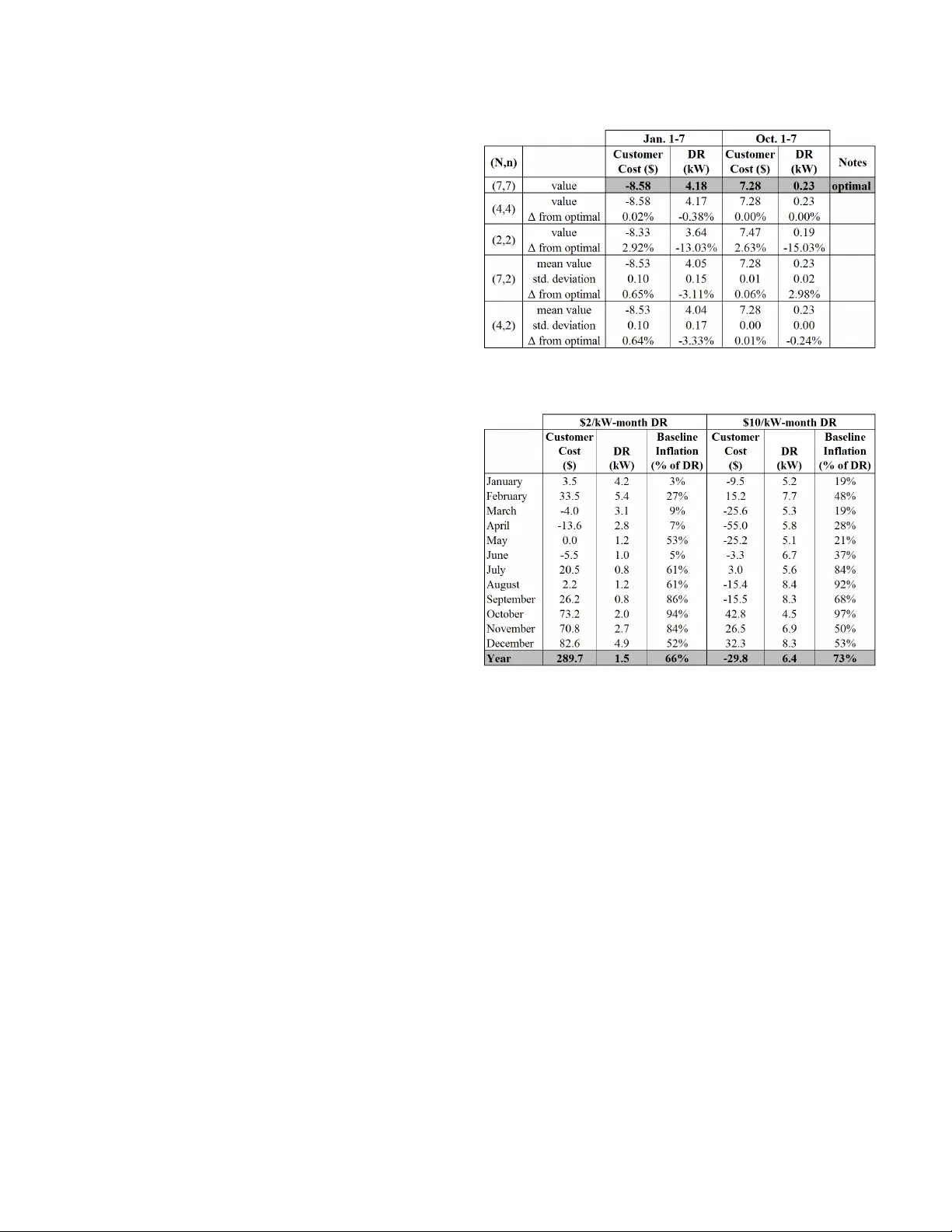
Model Pr edictiv e Contr ol-Based Battery Scheduling and Incentiv es to Manipulate Demand Response Baselines Douglas Ellman and Y uanzhang Xiao Abstract —W e study operations of a battery energy storage system under a baseline-based demand response (DR) program with an uncertain schedule of DR ev ents. Baseline-based DR programs may provide undesired incentives to inflate baseline consumption in non-event days, in order to increase “apparent” DR reduction in event days and secure higher DR payments. Our goal is to identify and quantify such incentives. T o understand customer decisions, we formulate the problem of determining hourly battery charging and discharge schedules to minimize expected net costs, defined as energy pur chase costs minus energy export rebates and DR payments, over a sufficiently long time horizon (e.g., a year). The complexity of this stochastic optimization problem gr ows exponentially with the time horizon considered. T o obtain computationally tractable solutions, we propose using multistage model predictive control with scenario sampling. Numerical results indicate that our solutions ar e near optimal (e.g., within 3% from the optimum in the test cases). Finally , we apply our solutions to study an example residential customer with solar photovoltaic and battery systems participating in a typical existing baseline-based DR program. Results rev eal that ov er 66% of the a verage apparent load reduction during DR e vents could result from inflation of baseline consumption during non-event days. I . I N T RO D U C T I O N An important mechanism for improving reliability and re- ducing costs of the power grid is demand response (DR). Among the v arious DR mechanisms that have been proposed or implemented [1] [2], we can cate gorize most of them as price-based DR and incentive-based DR. Price-based DR uses time-varying electricity prices to encourage customers to reduce consumption when prices are high. Alternativ ely , incentiv e-based DR pays customers rebates based on partici- pation or performance in the DR program. This paper focuses on baseline-based DR [3]–[11], an important and widely-used class of incentiv e-based DR. Baseline-based DR is prev alent in practice, because it can be an opt-in program without changing customer electricity rates, thus making it easier to achiev e regulatory approv al. Baseline-based DR pays customers based on the difference between energy consumption during DR e vents and baseline consumption (e.g., average consumption during previous non- ev ent days). While baseline-based DR gives customers incenti ves to reduce load during DR e vents, it may also create undesired incentiv es for customers to manipulate baselines. Randomized control trials [12] and legal settlements [13] have provided real-world e vidence that customers may manipulate baselines. In the past, manipulating DR baselines may have required substantial customer effort or diminished customer comfort The authors are with Hawaii Advanced W ireless T echnologies Institute and Department of Electrical Engineering, Uni versity of Hawaii at Manoa, Honolulu, HI 96822, USA. Email: { dellman, yxiao8 } @hawaii.edu. (e.g., manually changing air conditioner settings). But today , battery systems with automated controllers can optimize cus- tomer load profiles to maximize DR revenues with minimal customer ef fort and discomfort. Thus, customers with batter- ies may automatically use sophisticated strategies to exploit incentiv es to manipulate baseline load, perhaps without being aware that they are doing so. These behaviors may cause the utility to make significant errors in projecting demand forecasts, required DR quantities, and DR costs. Therefore, it is important to identify such behaviors and quantify their impacts. T o identify and quantify incenti ves to manipulate base- lines, we need to understand how the customer schedules hourly battery charging and discharging when participating in baseline-based DR programs ov er a suf ficiently long time horizon (e.g., a year), facing the uncertainty in when will the DR events occur . W e model the customer’ s decisions as solutions to a stochastic optimization problem of minimizing the e xpected net costs, defined as the energy purchase costs minus energy export payments and DR payments. Ho wev er, the stochastic optimization problem is intractable to solve, because its complexity grows exponentially with the time horizon. W e propose a multistage model predictiv e control (MPC) approach, which determines the battery schedule of each day by solving a stochastic program over a much shorter receding horizon (e.g., a month). Through simulations, we demonstrate that our proposed solutions are near optimal (e.g., within 3% from the optimum in the test cases). Then we apply our solutions to study an e xample residential customer with solar photo voltaic and battery systems participating in a typical existing baseline-based DR program. Results indicate that ov er 66% of the average apparent load reduction during DR ev ents could result from inflation of baseline consumption during non-ev ent days. W e summarize our major contributions as follo ws: • our work is the first to study incentiv es to manipulate DR baselines by using a battery; • our work introduces a stochastic optimization problem formulation, which is general enough to model a variety of baseline-based DR mechanisms over a long time horizon with uncertain DR e vent schedules; • our work proposes a computationally-tractable and near - optimal solution to the problem formulated, which allows us to identify and quantify customer incentives. The remainder of this paper is organized as follows: Section II discusses related work, Section III describes the problem, Section IV describes our solution, Section V describes a numerical case study for an example Honolulu residential customer , and Section VI summarizes conclusions. I I . R E L A T E D W O R K There is a huge literature on optimal battery dispatch under price-based DR (see some representative works in [14]–[18]). Some of these works use solution concepts similar to ours, namely stochastic programming and model-predictive control. Howe ver , since baselines are not part of price-based DR, these works do not study incenti ves to game baselines. Some works study optimal battery dispatch under baseline- based DR, but use pre-established baselines as inputs to their models [9]–[11]. These works essentially assume that the customer does not have the ability to manipulate the baseline, and therefore do not study incentiv es to game baselines. Many of the w orks that study gaming beha vior focus on mechanism design of the DR program [3]–[6]. In [4]– [6], customers self-report baselines, and truthful reporting is encouraged by excluding a subset of customers from each ev ent, and imposing penalties for deviations from reported baselines for those non-participating customers. In [3], there is a profit-sharing mechanism designed to discourage manip- ulating baselines for a DR program in which the baseline is the load at the start of the DR event. These works propose new DR mechanisms and do not model battery operations. In contrast, our work studies optimal battery operations under more commonly used e xisting DR mechanisms. The most related works are [7] [8], which study gaming incentiv es in baseline-based DR. The work in [7] only includes results for a two-stage model, where the second stage is the ev ent day with certainty . In comparison, our work considers uncertain event schedules ov er many days. Our prior work [8] studies a multi-day DR season with uncertain DR event sched- ules. It uses dynamic programming with backwards induction to obtain optimal energy consumption during DR windo ws of ev ent and non-event days, where there is a discrete set of daily feasible consumption le vels and the costs of realizing those consumption lev els are kno wn and independent of actions on other days. In contrast, our current work considers a battery system, where the feasible hourly char ging and discharging quantities and associated opportunity costs depend on actions taken at other times, and the action space is continuous. W e use model predictiv e control (MPC) to get a near-optimal battery dispatch, because the complexity of the model in [8] grows polynomially with the granularity of the discretization of inherently continuous action and state spaces, while our MPC approach allows continuous states and actions for free. Additionally , this work adds representation of DR mechanisms where payments depend on av erage power (kW) reduction ov er multiple ev ents (DR capacity payments). DR capacity payments could not be easily considered by the model in [8] because it would require significantly enlarging the state space to include information about prior ev ents. I I I . S Y S T E M M O D E L A N D P RO B L E M F O R M U L A T I O N A. Model Setup W e consider a customer with electric loads, a solar pho- tov oltaic system, and a battery energy storage system. The customer participates in a baseline-based demand response program and is subject to a certain electricity tarif f. W e look at a finite horizon of T days, where each day is index ed by t ∈ { 1 , . . . , T } . Due to the structure of the DR payments, these T days are di vided into I intervals (e.g., 12 months). The time- granularity of the battery charging and discharging decisions considered here is one hour, where each hour is indexed by h ∈ { 1 , . . . , H = 24 · T } . As will be useful later , we write t i as the final day of each interval i ∈ { 1 , . . . , I } , and h t as the final hour of each day t ∈ { 1 , . . . , T } . Our objecti ve is to determine the optimal schedule of battery char ging and discharging in each hour to minimize the expected total net cost for the customer ov er the T days. The demand response program aims to incentivize the cus- tomer to reduce electricity consumption during a pre-specified window of hours (e.g., 5 p.m – 9 p.m.) on demand response event days . Prior to any day , there is uncertainty on whether that day is an event day . This uncertainty can be represented by a Bernoulli random variable ω t with parameter P t , where ω t = 1 indicates that day t is an event day , and the probability that day t is an ev ent day is P t . W e assume that the random variables ω 1 , . . . , ω T are independent. At the beginning of each day , the customer is notified whether the current day is an event day . In each hour h , the customer has default electricity demand d h and solar ener gy production ρ h . The customer can charge the battery by an amount of b + h ≥ 0 or discharge the battery by an amount of b − h ≥ 0 , resulting in an hourly net load l h = d h + b + h − ρ h − b − h . Positiv e values of l h indicate that the customer purchases energy from the grid during hour h , and ne gati ve values indicate that the customer exports energy to the grid. The values d h , ρ h , b h , and l h are in the unit of kWh. The battery scheduling variables b + h and b − h are constrained by the physical characteristics of a battery system. A po wer capacity constraint requires the total amount of energy charged and dischar ged to be no lar ger than the rated power capacity P of the battery system in all hours, namely b + h + b − h ≤ P , ∀ h ∈ { 1 , . . . , H } . (1) W e denote the lev el of stored energy at each hour h by e h . The dynamics of the stored energy can be written as e h = e h − 1 + b + h · η + − b − h /η − , ∀ h ∈ { 2 , . . . , H } , (2) where η + ∈ (0 , 1) is the battery charging efficiency and η − ∈ (0 , 1) is the battery dischar ging ef ficiency . Finally , an energy capacity constraint requires that the lev el of stored energy does not exceed the rated ener gy capacity E of the battery system in all hours, namely 0 ≤ e h ≤ E , ∀ h ∈ { 1 , . . . , H } . (3) W e define b + t = ( b + h t − 1 +1 , . . . , b + h t ) as the vector of battery charging schedules in day t , and b − t = ( b − h t − 1 +1 , . . . , b − h t ) as the vector of battery dischar ging schedules in day t . B. Costs and P ayments The customer’ s economic incentiv es consist of costs and payments. The cost is the customer’ s energy purchase cost. For each hour when the net load is positi ve (i.e., l h > 0 ), the customer incurs an ener gy purchase cost c h , calculated as c h  b + h , b − h  = r c h · l h = r c h ·  d h + b + h − ρ h − b − h  , (4) where r c h is the electricity purchase rate per kWh for hour h . The payments come from energy export and the DR pro- gram. F or each hour when the net load is negati ve (i.e., l h < 0 ), the customer exports energy to the grid and receiv es an energy export payment p e h , calculated as p e h  b + h , b − h  = r e h · ( − l h ) = r e h ·  − d h − b + h + ρ h + b − h  , (5) where r e h is the electricity e xport rate per kWh for hour h . Additionally , the customer may receiv e DR energy pay- ments or DR capacity payments or both via the demand response program. Both types of DR payments are based on the quantity of demand response energy reduction, which is the dif ference between the true energy consumption and the baseline energy consumption during the DR window . W e write H t as the set of hours in the DR windo w of day t . Then the true energy consumption during the DR window of day t , denoted by s t , is calculated as s t = X h ∈H t l h . (6) At an e vent day t , the baseline consumption is calculated based on the consumption during the DR windo ws of a number of previous non-event days. W e write T B t as the set of non- ev ent days that affect the baseline in the e vent day t . Then the baseline ener gy consumption in an event day t , denoted by ¯ s B t , is defined as ¯ s B t = f ( { s τ } τ ∈T B t ) . (7) Usually , the baseline is simply the a verage consumption during the DR windo ws of rele vant non-e vent days (e.g. [19]), namely ¯ s B t =  P τ ∈T B t s τ  /   T B t   . Giv en the true and baseline consumption, the DR energy reduction in ev ent day t , denoted by ∆ t , can be calculated as ∆ t = ¯ s B t − s t . (8) Note that we allo w the reduction to be negati ve, so the customer could potentially pay a penalty for increasing the demand, as in [19]. Other programs do not penalize the customer for increasing the demand, in which case we will hav e ∆ t = max  0 , ¯ s B t − s t  . As in [20], the DR energy payment for each ev ent day t , denoted by p DR e t , is calculated by p DR e t  b + 1: t , b − 1: t ; ω 1: t  = r DR e t · ∆ t , (9) where r DR e t is the DR payment rate per kWh for day t , b + 1: t = ( b + 1 , . . . , b + t ) and b − 1: t = ( b − 1 , . . . , b − t ) are the battery charging and discharging schedules from day 1 to day t , respectiv ely , and ω 1: t = ( ω 1 , . . . , ω t ) is the sequence of e vent indicators up to day t . The customer receiv es no DR energy payment on non-ev ent days. Remark 1 (Inter-T emporal Dependence): The DR energy payment for an ev ent day t could depend on the battery scheduling decisions in day 1 , if for example, days 2 to t − 1 are all e vent days. W e write p DR e t  b + 1: t , b − 1: t ; ω 1: t  to explicitly indicate the inter-temporal dependence of the payment on the scheduling decisions. Strictly speaking, the DR energy payment depends only on the hours in the DR windows of previous days. But we use battery scheduling decisions of all previous hours b + 1: t and b − 1: t to simplify notations. Remark 2 (Randomness): In (9), we also make it clear that the DR payment p DR e t depends on the realization ω 1: t of the ev ent days from day 1 to day t , and therefore is random. This is because the set T B t of non-e vent days that af fect the baseline in day t depends on ω 1: t and is random. As a consequence, all the quantities related to DR ev ents, namely s t , ¯ s B t , ∆ t , and p DR e t depend on ω 1: t and are random. Another type of DR payment is the DR capacity payment, which is based on the average energy reduction per hour during an interval of days (e.g., a month). W e write the set of ev ent days in interv al i as T E i . Then the average energy reduction per hour during interval i , denoted by ¯ ∆ i , is calculated as ¯ ∆ i = P t ∈T E i ∆ t P t ∈T E i |H t | . (10) As in [20], the DR capacity payment during interv al i is then p DR c i  b + 1: t i , b − 1: t i ; ω 1: t i  = r DR c i · ¯ ∆ i , (11) where r DR c i is the DR capacity payment rate for interval i , and b + 1: t i and b − 1: t i are the battery char ging and discharging schedules from day 1 to the final day t i of interval i , and ω 1: t i = ( ω 1 , . . . , ω t i ) is the sequence of event indicators up to the final day t i of interval i . Again in (11), we make it clear that the DR capacity payment p DR c i depends on prior scheduling decisions and is random, as explained in Remarks 1 – 2. If there is no DR event during interval i , we set ¯ ∆ i = 0 . Note that some DR programs do giv e DR capacity payments (e.g., the prior interv al’ s amount) in the case of no ev ent. C. Pr oblem F ormulation W e aim to minimize the customer’ s expected total net cost ov er a finite time horizon of I intervals (e.g., 12 months), which consist of T days (e.g., 365 days), or equiv alently , H = 24 · T hours (e.g., 8760 hours). The decision variables are battery scheduling v ariables b + 1: T and b − 1: T during this time horizon. As sho wn in (9) and (11), the DR payments depend on the realization of random ev ent days. Therefore, the battery schedules b + t and b − t in day t should also depend on the previous and current realizations ω 1: t of ev ent days (but not future realizations due to causality). T o make this dependence explicit, we write the battery schedules as functions of the realizations, namely b + t ( ω 1: t ) and b − t ( ω 1: t ) . Giv en realizations of all events ω 1: T , the total net cost is C   b + t ( ω 1: t ) , b − t ( ω 1: t )  T t =1 ; ω 1: T  (12) = H X h =1 ( c h − p e h ) − I X i =1 p DR c i  b + 1: t i ( ω 1: t ) , b − 1: t i ( ω 1: t ); ω 1: t i  − I X i =1 X t ∈T E i p DR e t  b + 1: t ( ω 1: t ) , b − 1: t ( ω 1: t ); ω 1: t  . Our goal is to minimize the expectation of the abov e cost: minimize E ω 2: T n C   b + t ( ω 1: t ) , b − t ( ω 1: t )  T t =1 ; ω 1: T o subject to: under each ω 2: T ∈ { 0 , 1 } T − 1 , for t = 1 , . . . , T and h = h t − 1 + 1 , . . . , h t : b + h ( ω 1: t ) + b − h ( ω 1: t ) ≤ P , e h ( ω 1: t ) = e h − 1 ( ω 1: t ) + b + h ( ω 1: t ) · η + − b − h ( ω 1: t ) /η − , 0 ≤ e h ( ω 1: t ) ≤ E , variables: under each ω 2: T ∈ { 0 , 1 } T − 1 , b + t ( ω 1: t ) and b − t ( ω 1: t ) , t = 1 , . . . , T . (13) Note that the expectation is taken over the random ev ent schedules starting from day 2, namely ω 2: T , instead of ω 1: T . In practice, a customer is notified whether the next day is an ev ent day at least a few hours ahead. Therefore, at the time of solving the problem, we already know the realization of ω 1 . The problem in (13) is a multi-stage stochastic decision problem. The numbers of decision variables and constraints are lar ge and gro w exponentially with the length of the time horizon. More specifically , for each day t ∈ { 1 , . . . , T } , there are 2 t − 1 different scenarios (i.e., dif ferent realizations of ω 2: t ), and therefore 2 t − 1 different battery schedules b + t ( ω 1: t ) and b − t ( ω 1: t ) . So the total number of decision v ariables is 2 · 24 ·  1 + 2 + · · · + 2 T − 1  = 48 ·  2 T − 1  . For a one-year time horizon (i.e., T = 365 ), there are ov er 10 111 decision variables. The number of constraints gro w exponentially with the time horizon in the same way . In summary , it is impossible to obtain the exact solution to (13) under any reasonable length of time horizon. In the next section, we show how to obtain a near -optimal solution. I V . P R O P O S E D S O L U T I O N Since it is impractical to obtain the e xact solution to (13), we get near-optimal solutions by a multistage model predictiv e control approach with a receding horizon of N days, where N ≤ T . Specifically , for each day t , we solve a stochastic program that minimizes the customer’ s total cost from day t to day t + N − 1 , and obtain the battery schedules { b + τ , b − τ } t + N − 1 τ = t . W e use the decisions b + t , b − t for the day t only . For the next day t + 1 , we solve a stochastic program that minimizes the cost from day t + 1 to day t + N , in order to get the schedules b + t +1 , b − t +1 . W e repeat this process for each day . The hypothesis behind this approach is that when the receding horizon N is sufficiently large, the current day’ s action is less likely to affect the costs more than N days in ω t : ω t +1 : ω t +2 : ω t +3 : ω t +4 : 1 0 1 0 1 0 1 0 1 0 1 0 1 0 1 0 1 0 1 0 1 0 1 1 0 1 0 1 0 1 0 perfect binary tree of depth 2 sampled branch: e ω t +2: t +4 (10) sampled branch: e ω t +2: t +4 (11) Fig. 1. An example of the binary scenario tree. Day t is an event day , the receding horizon is N = 5 , all possible scenarios ω t : t +1 in the first n = 2 days are ev aluated, and one scenario e ω t +2: t +4 ( ω t : t +1 ) from day t + 2 to day t + 4 is sampled after each ω t : t +1 . the future. Therefore, the battery schedules obtained from the stochastic program ov er the smaller time horizon of N days are likely to be close to the optimal schedules. Since the receding horizon (e.g., N = 30 days) can be much smaller than the entire time horizon (e.g., T = 365 days), we solve a much smaller problem than (13). In addition to using a receding horizon of N days, we further simplify the stochastic program by approximating the objectiv e function in (13) through sampling. The objectiv e function in (13) is the expected net cost, where the expectation is taken over the random event schedules ω 2: T . Such an expectation is computed as the weighted sum of net costs in 2 T − 1 different scenarios , where each scenario is a realization ω 1: T . In the multistage model predictive control approach outlined abov e, we limit the lookahead horizon to N days, and take the expectation over the realization ω t +1: t + N − 1 (we already know ω t when solving the problem). Therefore, we need to ev aluate 2 N − 1 scenarios. Although we ha ve N < T , the number of scenarios may still be large. This motiv ates us to further reduce the number of scenarios to consider . T o better explain our approach, we can define a binary scenario tr ee to represent the scenarios to e valuate. The root indicates whether day t is an ev ent day , and the two child nodes of the root represent the two possibilities that day t + 1 is an ev ent day or a non-event day . In general, there are 2 τ − 1 nodes of depth τ ≥ 2 , representing the possibilities of day t + τ − 1 following the 2 τ − 2 scenarios ω t : t + τ − 2 from day t to day t + τ − 2 . W e will hav e a perfect binary tree of depth n ≤ N , in which all interior nodes hav e two children and all leav es have the same depth. Then each leaf node of this n -le vel perfect binary tree has one deg enerate branch of depth N − n , namely a branch in which all interior nodes ha ve exactly one child. Each degenerate branch corresponds to the selection of one scenario out of 2 N − n scenarios ω t + n : t + N − 1 from day t + n to day t + N − 1 . W e select the scenario by sampling according to the probabilities that each scenario occurs, where the probability of the scenario ω t + n : t + N − 1 is t + N − 1 Y τ = t + n (1 − P τ ) 1 − ω τ ( P τ ) ω τ (14) T o define the reformulated problem to solve, for each τ ≥ t + n , we write e ω t + n : τ ( ω t : t + n − 1 ) as the sampled realization of ev ent days from day t + n to day τ given the realization ω t : t + n − 1 of ev ent days from day t to day t + n − 1 . W e write it as function of ω t : t + n − 1 , because we need to sample one scenario after each ω t : t + n − 1 . In the scenario tree, the selected e ω t + n : t + N − 1 ( ω t : t + n − 1 ) is the degenerate branch spa wning from the leaf node of the branch ω t : t + n − 1 in the perfect binary tree of depth n . Note that e ω t + n : t + N − 1 ( ω t : t + n − 1 ) is random. For each τ ≥ t + n , we write e ω t : τ ( ω t : t + n − 1 ) as the concatenation of ω t : t + n − 1 and e ω t + n : τ ( ω t : t + n − 1 ) . Based on the above notations, we can write the decision variables in the multistage MPC problem as under each ω t +1: t + n − 1 ∈ { 0 , 1 } n − 1 , (15) for τ = t, . . . , t + n − 1 : b + τ ( ω t : τ ) , b − τ ( ω t : τ ) , for τ = t + n, . . . , t + N − 1 : b + τ [ e ω t : τ ( ω t : t + n − 1 )] , b − τ [ e ω t : τ ( ω t : t + n − 1 )] . In other words, we need to determine the battery schedules under all possible scenarios from day t + 1 to day t + n − 1 , and the schedules under only sampled scenarios from day t + n to day t + N − 1 . Hence, we limit the number of v ariables to 2 · 24 ·  1 + 2 + · · · + 2 n − 1 + 2 n − 1 · ( N − n )  = 48 ·  2 n − 1 · ( N − n + 2) − 1  . (16) W e can see that the number of decision v ariables does not depend on the full length T of the time horizon, and gro ws linearly with the receding horizon N and exponentially with n . W e control the complexity of the MPC problem through n . Next, we define the modified net cost over the receding horizon. W e write I t as the set of intervals included in the receding time horizon from day t to day t + N − 1 . F or example, if N = 20 and each interval is a month, then I 1 = { 1 } and I 15 = { 1 , 2 } . Dropping the dependence of the decision variables on the scenarios for notational simplicity , we can write the modified net cost as e C t   b + τ , b − τ  t + N − 1 τ = t ; ω t : t + n − 1  (17) = h t + N − 1 X h = h t − 1 +1 ( c h − p e h ) − X i ∈I t ˜ p DR c i  b + t : t + N − 1 , b − t : t + N − 1 ; ω t : t + n − 1  − X i ∈I t X τ ∈T E i ∩ [ t,t + N − 1] p DR e τ  b + t : τ , b − t : τ ; ω t : t + n − 1  , where the energy purchase cost c h , the energy export payment p e h , and the DR energy payment p DR e τ remain the same as in (12), but the DR capacity payment ˜ p DR c i is the approximation of the true DR capacity payment p DR c i . In our MPC approach, we may not be able to compute the true DR capacity payment, because the receding horizon may end before the end of an interval. Since we do not kno w the demand reduction in the remaining days of this interval, we cannot compute the av erage demand reduction in this interv al and the true DR capacity payment. In this case, we calculate the DR capacity payment p DR c i of interval i according to (11) ov er interval i ’ s days before the end of the horizon, and then discount it by the fraction of total days in the interv al that are considered, namely ˜ p DR c i = min { t i , t + N − 1 } − t i − 1 t i − t i − 1 · p DR c i . (18) W e discount the DR capacity payment, because the tariff costs and DR energy payments are calculated ov er a fraction of the month, and we want to use a corresponding portion of the total DR capacity payment over the month. If the receding horizon starts after the start of an interval, we use stored values of demand reductions in event days prior to the current receding horizon. Finally , it is worth to note that the modified cost e C t  { b + τ , b − τ } t + N − 1 τ = t ; ω t : t + n − 1  is random, because we ran- domly select the scenario e ω t + n : t + N − 1 ( ω t : t + n − 1 ) after day t + n − 1 . Now we can formulate the problem to solve in our MPC approach as follows. min E ω t +1: t + n − 1 n e C t   b + τ , b − τ  t + N − 1 τ = t ; ω t : t + n − 1 o s.t. under each ω t +1: t + n − 1 ∈ { 0 , 1 } n − 1 , for τ = t, . . . , t + n − 1 , and h = h τ − 1 + 1 , . . . , h τ : b + h ( ω t : τ ) + b − h ( ω t : τ ) ≤ P , e h ( ω t : τ ) = e h − 1 ( ω t : τ ) + b + h ( ω t : τ ) · η + − b − h ( ω t : τ ) /η − , 0 ≤ e h ( ω t : τ ) ≤ E , for τ = t + n, . . . , t + N − 1 and h = h τ − 1 + 1 , . . . , h τ : b + h [ e ω t : τ ( ω t : t + n − 1 )] + b − h [ e ω t : τ ( ω t : t + n − 1 )] ≤ P , e h [ e ω t : τ ( ω t : t + n − 1 )] = e h − 1 [ e ω t : τ ( ω t : t + n − 1 )] + b + h [ e ω t : τ ( ω t : t + n − 1 )] · η + − b − h [ e ω t : τ ( ω t : t + n − 1 )] /η − , 0 ≤ e h [ e ω t : τ ( ω t : t + n − 1 )] ≤ E , variables: as defined in (15) . (19) Similar to (13), we take the expectation over the random ev ent schedules starting from day t + 1 , namely ω t +1: t + n − 1 , because we already know the realization of ω t when solving the problem for day t . Remark 3 (Appr oximation and Randomness): Note that the objectiv e function and decision variables in the proposed MPC approach (19) are dif ferent from those in the original scheduling problem (13). For computational feasibility , we reduce the number of decision variables by reducing the time horizon and ev aluating only selected scenarios, and make necessary approximations in the cost function due to the reduced time horizon. Therefore, the proposed solution (19) is an approximation to the optimal solution to (13). W e can recov er the optimal solution by setting the time horizon the same as that in the original problem (i.e., N = T ) and minimizing the exact expected cost (i.e., n = N ). Note also that the objective function and the constraints in (19) are random due to the randomly sampled e ω t + n : t + N − 1 ( ω t : t + n − 1 ) after each ω t : t + n − 1 (ev en though we take the expectation ov er ω t +1: t + n − 1 ). Therefore, the solution, namely the bat- tery schedules, is random and depends on which scenario e ω t + n : t + N − 1 ( ω t : t + n − 1 ) was sampled. In Section V -B, we study the effect of random sampling numerically and find it to be negligible for the cases we inv estigated. W e will also study the suboptimality introduced by limiting the time horizon to N in the next section. V . C A S E S T U DY In this section, we apply the model and the solution in Section III and Section IV to an example residential customer participating in a tariff and DR program based on the existing Customer Grid Supply Plus tarif f [21] and the Capacity Reduction Grid Service DR program [19] 1 . W e first study several cases whose time horizons are small enough for us to compute the optimal solutions, and compare our proposed solutions with the optimal solutions. Next, we present numerical results for a case study with a full-year time horizon, in order to identify customer incenti ves to increase baseline energy consumption. A. Basic Simulation Setup W e first describe the parameters that are common to all of the cases. 1) Customer default electricity demand: The default cus- tomer electricity demand is the base-case Honolulu residential customer demand obtained from an OpenEI dataset [22], which includes synthesized hourly load profiles for a typical year’ s weather corresponding to the T ypical Meteorological Y ear 3 (TMY3) dataset [23]. 2) Solar photovoltaic energy production: The solar produc- tion is obtained from PVW atts [24], based on a 9.5 kW rooftop system with default parameters and the Honolulu TMY3 weather data. Using TMY3 data for both customer demand and solar aligns their weather-based variations. The solar system size was selected so that annual production roughly matches annual customer demand. 3) Battery ener gy stora ge system: The customer’ s battery consists of two units of the T esla Powerwall battery [25], a popular residential battery system. The round-trip efficienc y is 90%. Assuming equal charging and discharging efficiency , we ha ve η + = η − = √ 0 . 9 . The total battery system po wer capacity is 10 kW and energy capacity is 27 kWh. The battery energy capacity was selected to be similar to the customer’ s daily energy demand. 4) Customer tariff: The customer receives $0.108/kWh for energy exported to the grid, and the customer pays $0.29/kWh to purchase energy from the grid. The difference between the export rate and the purchase rate incentivizes charging the battery when solar production exceeds load, and discharging that energy later to reduce grid purchases. 1 This case study simplifies some elements of the Customer Grid Supply Plus tariff and the Capacity Reduction grid service, but aims to represent the major elements that could lead to incentives to game baselines. For example, Capacity Reduction includes separate payments to aggregators and customers, but this study considers that the aggregator and customers act as one entity . Interested readers can refer to the program documents for more information. 5) DR pr ogram details: The customer recei ves a DR ca- pacity payment based on av erage load reduction during DR ev ents each month. The DR window is from 5 p.m. to 9 p.m. in all ev ent days. Baseline energy consumption is the average energy consumption during the DR windows of some number of previous non-e vent days. 6) Pr obabilities of DR events: The probabilities of a DR ev ent occurring each day were calculated based on a logistic regression of occurrence of a DR ev ent versus daily peak temperature. The logistic regression model was created based on 2017 Hawaiian Electric system electricity demand [26] and 2017 weather data for Honolulu [27]. Capacity Reduction DR ev ents can be called up to 104 times per year [19], so e vent days were assigned to the 104 days of 2017 with the highest peak hourly electricity demand. A logistic regression model of DR ev ent occurrence versus daily peak temperature was used to calculate daily ev ent probabilities for Honolulu TMY3 weather . 7) Initial values: For the first day , the initial battery state of charge is set to 50% of the battery energy capacity , and the initial baseline is set to all zeros. B. Assessing The Quality of Pr oposed Solutions As explained in Remark 3, our proposed solution is an ap- proximation to the optimal solution, and is random. Therefore, it is important to assess its performance in terms of the cost and its variance. T o compare with the optimal solution, we need to restrict to cases whose time horizons are small enough so that it is feasible to compute the optimal solution. W e consider a time horizon of T = 7 days, which is long enough to sho w multi-day effects, and short enough to allo w computing the optimal solution. Due to the small number of days in these cases, we use a 3-day baseline (i.e., the baseline consumption is the average of previous 3 non-ev ent days), which is shorter than the standard 10-day baseline in Capacity Reduction. W e consider two periods of 7 days: the first 7 days in January (low temperature and low probabilities of e vents) and the first 7 days in October (high temperature and high probabilities of ev ents). W e set the rate r DR c i of DR capacity payments to be $2/kW (the minimum customer incentiv e lev el allowed for Capacity Reduction grid service [19]), and use the per-hour demand reduction av eraged ov er the 7 days, instead of over the entire month, to determine DR capacity payments. T able I presents the results for the 7-day case study in January and October . The table sho ws customer cost and demand response quantity , as expected values ov er the random ev ent schedules ω 1:7 . Additional metrics baseline load (i.e., av erage baseline load ov er all events in kW) and ev ent load (i.e., average load over all ev ents in kW) were also calculated. W e first show the metrics under the optimal solution, which is obtained by setting N = n = 7 . Then we ev aluate our proposed solution under different receding horizons of N = 4 and N = 2 without sampling (i.e., n = N in both cases). In these two cases with n = N , we optimize the expected cost over all ev ent schedules ω t : t + N − 1 , which results in deterministic solutions. In this way , we can focus on the impact of a shorter receding horizon. W e can see that under the 4-day receding horizon, customer cost nearly matches the optimal cost, and under the 2-day receding horizon, customer cost is about 3% higher than the optimal cost. This suggests that a shorter receding horizon can provide close to optimal results. As we would expect, the performance tends to improve with the length of the receding horizon. Next we focus on the impact of sampling the scenario tree. W e set the receding horizon as the entire time horizon (i.e., N = T = 7 ), consider all the possible scenarios in the first 2 days (i.e., n = 2 ), and sample one event schedule from day 3 to day 7 . In this case, the proposed solution depends on the sampled e vent schedule e ω 3:7 , and therefore, is random. W e run the simulations 5 times to get 5 battery schedules under different sampled ev ent schedules, and show the mean and the standard de viation of the performance metrics ov er these 5 runs. W e can see that the customer cost is within 1% of the optimum with small standard de viation. Finally , we set N = 4 and n = 2 to e valuate the proposed solution with both a shorter receding horizon and sampled event schedules. Again, since the proposed approach yields dif ferent battery schedules under dif ferent sampled ev ent schedules, we show the average metrics and standard deviations over 5 runs. The customer cost is within 1% of the optimum with small standard de viation. Comparing the cases of ( N , n ) = (7 , 2) and ( N , n ) = (4 , 2) with the case of ( N , n ) = (2 , 2) , we can see that under the same depth of the perfect binary tree (i.e., n = 2 ), we can improv e the performance (i.e., from about 3% within the optimum to within 1% from the optimum) by sampling additional days (i.e., 5 additional days when N = 7 and 2 additional days when N = 4 ). Compared to customer cost, the DR quantity metric tends to show greater percentage dif ferences from the optimal case. Howe ver , the values are still reasonably close to the optimal case in absolute magnitude and ha ve reasonably small standard deviations. This finding also holds for the baseline load and ev ent load metrics. Our conclusion from this study is that it is possible to significantly reduce the number of scenarios considered in the scenario tree and still obtain near-optimal results. W e thus use our proposed approach in the full-year study , where calculating the optimal solution is not feasible. C. Evaluating Customer Incentives W e study the battery scheduling problem with a time horizon of a full year (i.e., T = 365 ). In the proposed solution, we choose a receding horizon of N = 35 (longer than a full month, over which the DR capacity payment is calculated) and a depth n = 4 of the perfect binary scenario tree (based on results in T able I). W e consider two DR capacity payment rates of $2/kW and $10/kW . W e also create a “counter-f actual” case, as a control group, where the customer does not participate in the DR program. In this case the objective is to minimize net tariff costs (i.e., costs of ener gy purchase from the grid minus rebates for exports). The stochastic parameters representing ev ent schedule do not impact this cost, so the optimal decisions for this case can be T ABLE I A P PR OX I MATI O N S T U DY R E S ULT S T ABLE II F U LL - Y E AR R E SU LT S solved in a single scenario. Ho wever , in the counter -factual case, there are many dif ferent solutions that yield the same optimal cost with varying lev els of electricity consumption during DR windows. In order to compare e vent and baseline load between the DR cases and the counter-factual case, we need to select one from multiple optimal solutions. For this study , we selected the optimal battery dispatch schedule that char ges the battery as much as possible to absorb solar energy that exceeds load, and dischar ges the battery as much as possible to avoid purchasing power from the grid. This schedule was selected because it is a realistic and simple algorithm to implement on batteries that are deployed today , and thus represents a plausible counter-factual case. T able II sho ws results for the cases with $2/kW -month and $10/kW -month DR capacity payments. In addition to the metrics shown, we also calculated average baseline load and ev ent load. Since the proposed approach yields stochastic solutions that depend on the sampled schedules, we run the experiments 10 times to get the mean v alues of the metrics. F or these cases we calculate the baseline inflation (the difference between baseline load with DR payments and baseline load in the case with no DR payment), and use this to calculate “Baseline Inflation (% of DR), ” which shows the portion of apparent DR load reduction is actually due to baseline inflation. In the “counter-factual” case with no DR payments, av erage baseline load and event load for the year are both approxi- mately 0.1 kW , and average DR quantity is approximately 0.0 kW . This reflects that when the battery is used to minimize tariff costs via our heuristic, the battery covers most of the load during the DR windo ws of 5 p.m. to 9 p.m.. There is not a significant difference in DR window energy consumption between ev ent and non-event days. The $2/kW -month case sho ws higher baseline load (1.1 kW) and lower event load (-0.4 kW). This indicates that while the DR program does incenti vize the customer to reduce load during events, it also incentivizes e ven greater increases in energy consumption during DR windows of non-e vent days. Over the year , 66% of the apparent DR is due to baseline inflation, with monthly values ranging from 3% in January to 94% in October . The $2/kW -month case also indicates that e ven at the minimum payment lev el, the Capacity Reduction grid service successfully provides an incentiv e for the customer to modify battery charging to deliv er DR. Comparing the quantity of av erage DR (1.5 kW) to the size of the battery system (10 kW , 27 kWh), we see that the quantity of DR is much smaller than what could be obtained if the battery was solely focused on deliv ering DR. This reflects that at this relatively lo w DR payment lev el, the battery often prioritizes the high-value application of shifting solar production to reduce tarif f costs. The $10/kW -month case shows e ven higher baseline load (4.8 kW) and lower event load (-1.7 kW), indicating stronger incentiv es to reduce load during e vents and increase load during DR windo ws of non-ev ent days. Over the year , 73% of the apparent DR is due to baseline inflation, with monthly values ranging from 19% in January and March to 97% in October . While the ov erall trend w as to increase the percentage of baseline inflation compared to the $2/kW -month case, in some months (May , September , November) the percentage of baseline inflation was lower . This is because the relationship between DR payment and strength of incentiv es to lo wer ev ent load and increase baseline load can vary based on monthly parameters including event probabilities, customer default demand, and solar ener gy production. R E F E R E N C E S [1] J. S. V ardakas, N. Zorba, and C. V . V erikoukis, “A Survey on Demand Response Programs in Smart Grids: Pricing Methods and Optimization Algorithms, ” IEEE Communications Surveys and T utorials , vol. 17, no. 1, pp. 152–178, 2015. [2] B. Chew , B. Feldman, D. Ghosh, and M. Surampudy , “2018 Utility Demand Response Market Snapshot, ” Smart Electric Po wer Alliance, T ech. Rep., 2018. [Online]. A vailable: https://sepapower .org/resource/ 2018- demand- response- market- snapshot/ [3] D. G. Dobakhshari and V . Gupta, “A Contract Design Approach for Phantom Demand Response, ” IEEE T ransactions on Automatic Contr ol , p. 1, 2018. [4] D. Muthirayan, E. Baeyens, P . Chakraborty , K. Poolla, and P . P . Khargonekar , “A Minimal Incentive-based Demand Response Program W ith Self Reported Baseline Mechanism, ” 2019. [Online]. A v ailable: https://arxiv .org/pdf/1901.02923.pdf [5] D. Muthirayan, D. Kalathil, K. Poolla, and P . V araiya, “Mechanism de- sign for demand response programs, ” arXiv preprint , 2017. [6] J. V uelvas, F . Ruiz, and G. Gruosso, “Limiting gaming opportunities on incentiv e-based demand response programs, ” Applied Energy , vol. 225, pp. 668–681, sep 2018. [7] J. V uelvas and F . Ruiz, “Rational consumer decisions in a peak time rebate program, ” feb 2018. [Online]. A vailable: http: //arxiv .org/abs/1802.08112 [8] D. Ellman and Y . Xiao, “Customer Incenti ves for Gaming Demand Response Baselines, ” in Accepted by 58th IEEE Conference on Decision and Contr ol , 2019. [9] S. Bruno, G. Giannoccaro, and M. L. Scala, “Optimization of residential storage and energy resources under demand response schemes, ” in 2018 19th IEEE Mediterranean Electr otechnical Confer ence (MELECON) . IEEE, may 2018, pp. 225–230. [10] K. Garifi, K. Baker , B. T ouri, and D. Christensen, “Stochastic Model Predictiv e Control for Demand Response in a Home Energy Manage- ment System, ” in 2018 IEEE P ower & Energy Society General Meeting (PESGM) . IEEE, aug 2018, pp. 1–5. [11] A. Castelo-Becerra, W . Zeng, and M.-Y . Chow , “Cooperative distributed aggregation algorithm for demand response using distributed energy storage devices, ” in 2017 North American P ower Symposium (NAPS) . IEEE, sep 2017, pp. 1–6. [12] F . W olak, “Residential Customer Response to Real-Time Pricing: The Anaheim Critical-Peak Pricing Experiment, ” 2006. [Online]. A vailable: https://escholarship.org/uc/item/3td3n1x1 [13] J. Pierobon, “T wo FERC settlements illustrate attempts to ‘game’ demand response programs, ” 2013. [Online]. A vail- able: https://www .theenergyfix.com/2013/07/25/two- ferc- settlements- illustrate- attempts- to- game- demand- response- programs/ [14] D. T . V edullapalli, R. Hadidi, and B. Schroeder , “Optimal Demand Response in a building by Battery and HV AC scheduling using Model Predictiv e Control, ” in 2019 IEEE/IAS 55th Industrial and Commercial P ower Systems T echnical Conference (I&CPS) . IEEE, may 2019, pp. 1–6. [15] E. Vrettos, K. Lai, F . Oldewurtel, and G. Andersson, “Predictive Control of buildings for Demand Response with dynamic day-ahead and real- time prices, ” in 2013 European Contr ol Conference (ECC) . IEEE, jul 2013, pp. 2527–2534. [16] C. Keerthisinghe, A. C. Chapman, and G. V erbi ˇ c, “Energy Management of PV -Storage Systems: Policy Approximations Using Machine Learn- ing, ” IEEE Tr ansactions on Industrial Informatics , vol. 15, no. 1, pp. 257–265, jan 2019. [17] X. Jin, K. Baker , S. Isley , and D. Christensen, “User-preference-driv en model predictive control of residential building loads and battery storage for demand response, ” in 2017 American Contr ol Confer ence (ACC) . IEEE, may 2017, pp. 4147–4152. [18] Y . Xu and L. T ong, “On the operation and value of storage in consumer demand response, ” in 53rd IEEE Conference on Decision and Control . IEEE, dec 2014, pp. 205–210. [19] Hawaiian Electric, “ Addendum No. 2 T o Request for Proposals For Provision of Grid Services Utilizing Demand-Side Resources, ” 2018. [Online]. A vailable: https: //www .hawaiianelectric.com/documents/products { } and { } services/ demand { } response/dr { } rfp { } best { } and { } final { } offer .pdf [20] Con Edison, “Commercial Demand Response Program Guidelines, ” 2019. [Online]. A vailable: https://www .coned.com/- /media/files/coned/ documents/sav e- energy- money/rebates- incenti ves- tax- credits/smart- usage- rew ards/smart- usage- program- guidelines.pdf?la=en [21] Hawaiian Electric, “Customer Grid-Supply Plus. ” [On- line]. A vailable: https://www .haw aiianelectric.com/products- and- services/customer- rene wable- programs/customer- grid- supply- plus [22] Office of Energy Efficiency & Renewable Energy (EERE), “Commercial and Residential Hourly Load Profiles for all TMY3 Locations in the United States. ” [Online]. A vailable: https://openei.org/doe- opendata/dataset/commercial- and- residential- hourly- load- profiles- for- all- tmy3- locations- in- the- united- states [23] National Renewable Energy Laboratory, “National Solar Radiation Data Base: 1991- 2005 Update: T ypical Meteorological Y ear 3. ” [Online]. A v ailable: https://rredc.nrel.gov/solar/old { } data/nsrdb/1991- 2005/tmy3/ [24] ——, “PVW atts Calculator. ” [Online]. A vailable: https://pvwatts.nrel. gov/pvwatts.php [25] T esla, “Powerwall — The T esla Home Battery. ” [Online]. A v ailable: https://www .tesla.com/powerwall [26] Federal Energy Regulatory Commission, “Form 714 - Annual Electric Balancing Authority Area and Planning Area Report. ” [Online]. A vailable: https://www .ferc.gov/docs- filing/forms/form- 714/data.asp [27] W eather Underground, “W eather History & Data Archive. ” [Online]. A vailable: https://www .wunderground.com/history/