Optimal Safe Controller Synthesis: A Density Function Approach

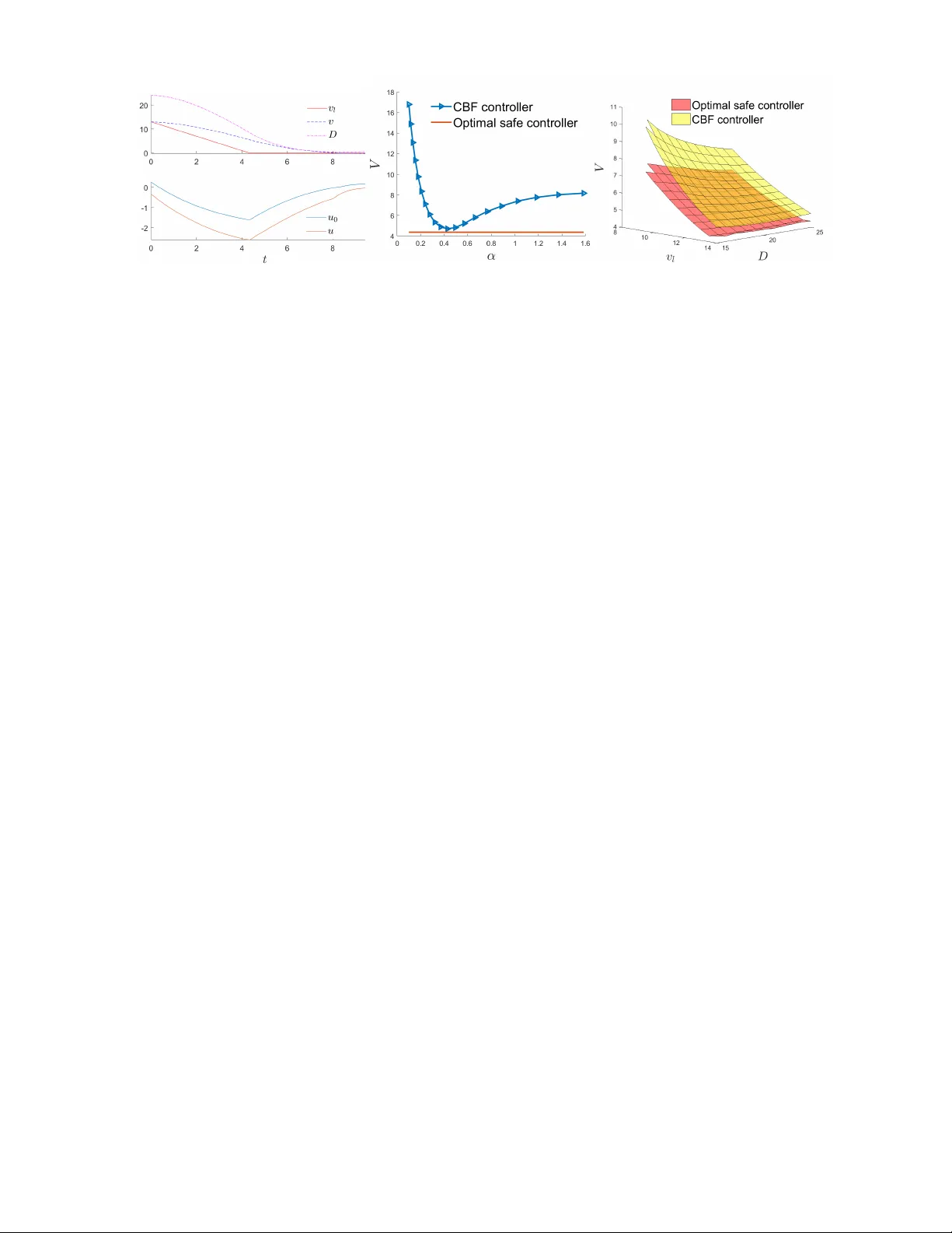
Optimal Safe Contr oller Synthesis: A Density Function A ppr oach Y uxiao Chen, Mohamadreza Ahmadi, and Aaron D. Ames Abstract — This paper considers the synthesis of optimal safe controllers based on density functions. W e present an algorithm for rob ust constrained optimal control synthesis using the duality relationship between the density function and the value function. The density function follo ws the Liouville equation and is the dual of the value function, which satisfies Bellman’s optimality principle. Thanks to density functions, constraints over the distribution of states, such as safety constraints, can be posed straightforwardly in an optimal control problem. The constrained optimal control problem is then solved with a primal-dual algorithm. This formulation is extended to the case with external disturbances, and we show that the robust constrained optimal control can be solved with a modified primal-dual algorithm. W e apply this formulation to the prob- lem of finding the optimal safe controller that minimizes the cumulative intervention. An adaptive cruise control (A CC) example is used to demonstrate the efficacy of the proposed, wherein we compare the result of the density function approach with the conv entional control barrier function (CBF) method. I . I N T RO D U C T I O N Safety is one of the fundamental goals of control syn- thesis. Controller design techniques, such as control barrier function (CBF) methods, hav e been proved to be powerful tools for guaranteeing safety of dynamical systems and their application spans over robotics [7], [10], [15], [21] and transportation systems [9], [16]. One of the strengths of the CBF is its ability to work with the legac y controller , e.g. a tracking controller, in a plug-and-play fashion. Giv en any legac y controller , the CBF acts as the supervisory controller, filtering the input from the legac y controller with minimum intervention necessary to guarantee safety . This supervisory control structure is sho wn in Fig.1. The computation of CBFs typically centers around in- variance conditions, which can be enforced via polytopic projection [16], robust optimization [8], and sum of squares constraints [22]. Howe ver , one ca veat of the CBF method is that it operates myopically , i.e., the CBF is a function of only the current state, and the intervention only depends on the current situation. Although the intervention at ev ery time instance is minimized, the cumulativ e intervention is not necessarily minimized. If a CBF controller is designed too conservati vely , it may use unnecessary intervention when the situation is not dangerous; if a CBF controller is too op- timistic, it may allow the state to get too close to the danger set and hav e to inv oke large intervention to prev ent the state from entering the danger set. Giv en a legac y controller, it is not clear how to synthesize the optimal safe controller that minimizes the cumulativ e intervention. Besides, the The authors are with the Department of Mechanical and Civil Engineer- ing, California Institute of T echnology , Pasadena, CA, 91106, USA. Emails: { chenyx, mrahmadi, ames } @caltech.edu Fig. 1: CBF as the supervisory controller computation of the CBF is nontrivial, almost all numerical methods suf fer from dif ferent lev els of conserv atism, which further compromises the performance. In terms of optimality , optimal control is one of the most well-studied problems in control. Bellman’ s principle of optimality [4] and Pontryagin’ s maximum principle [17] are two fundamental theories that solve optimal control problems. W ith Hamilton-Jacobi-Bellman (HJB) partial dif- ferential equation (PDE), we can ev en solve for the optimal control strategy for the whole state space [3]. Ho wev er, when there are safety constraints, such as those requiring that the state should nev er leave a set or enter a set, the HJB PDE cannot encode those constraints in a clear way . The constrained optimal control problem can be solved for a given initial condition with Lagrangian multipliers [5], but it only giv es solution to a single initial condition rather than the whole state space, and computing the solution online is typically not feasible due to the complexity . Density functions, proposed by Rantzer in [20], are the dual of L yapunov functions and can be used to verify the stability of nonlinear systems [18] as well as reachability analysis of polynomial systems [19]. One related concept is the occupation measure studied in [11]–[13], [23], which considers the dual relationship between functions and mea- sures and solve the optimal control problem with moment programming. W e recently showed in [6] that the density function is the dual of the value function in optimal control and one can enforce safety constraints on the density function and solv e the constrained optimal control problem with a primal-dual algorithm. In this paper , we take advantage of this duality relationship to design controllers that are both safe and optimal. Furthermore, we consider the case where the dynamical system is subject to exogenous disturbances and propose a synthesis procedure for controllers with safety and optimality . W e elucidate our proposed methodology with an adapti ve cruise control example. The rest of the paper is org anized as follo ws. In the next section, we revie w some preliminary notions and definitions used in the paper . In Section III, we discuss the duality between the density functions and the optimal control v alue functions. In Section IV, we propose a technique to syn- thesize controllers that guarantee safety and optimality . In Section V, we elucidate the efficacy of the proposed method- ology with an adapti ve cruise control e xample. Finally , in Section VI, we conclude the paper . Nomenclatur e N denotes the set of natural numbers, N + denotes the positiv e natural number , R denotes the set of real numbers. Giv en a differential equation ˙ x = f ( x ) , where f : X → R n is a locally Lipschitz function, Φ f ( x 0 , T ) denotes the flow map of the dynamics with initial state x 0 and horizon T . h a, b i X = R X a ( x ) · b ( x ) dx denotes the inner product of two functions a and b . 0 denotes a vector of all zeros or a function that is always zero, depending on the context. 1 S denotes the indicator function of a set S . W e use bold font u to denote a controller that maps state to the control input, and normal font u to denote the actual control input. For a variable x ∈ X , x [ · ] denotes its trajectory over time and X [ · ] denote the set of possible trajectories. I I . P R E L I M I NA R I E S In this section, we revie w several notion and definitions used throughout the paper . A. Density functions for dynamical systems Density function can be understood as the measure of state concentration in the state space. Gi ven a dynamical system ˙ x = f ( x ) , x ∈ X ⊆ R n , (1) the density function ρ : [0 , ∞ ) × X → R describes the concentration of states, and its e volution follo ws the Liouville PDE: ∂ ρ ∂ t + ∇ · ( ρ · f ) = φ ( t, x, ρ ) , ρ (0 , x ) = ρ 0 ( x ) , (2) where φ : [0 , ∞ ) × X × R → R is the supply function, φ ( t, x 0 , ρ ( x 0 , t )) > 0 denotes a source representing where the new states appear, and φ ( t, x 0 , ρ ( x 0 , t )) < 0 denotes a sink, indicating that some states exit the system at x 0 , time t . W e let φ depend on ρ to allow more flexible characterization of the supply . The Liouville PDE can be transformed and solved as an ordinary dif ferential equation (ODE) since ∂ ρ ∂ t + ∇ · ( ρ · f ) = dρ dt     ˙ x = f ( x ) + ( ∇ · f ) ρ = φ. (3) This implies that we can integrate the following ODE to get the density function alone the trajectory of the dynamic system ˙ x = F ( x ) as  ˙ x ˙ ρ  =  f ( x ) φ ( t, x, ρ ) − ∇ · f ( t, x ) ρ  . (4) Then, giv en an initial density distribution ρ (0 , · ) = ρ 0 and supply φ , the density at state x T , time T can be computed with the follo wing two step process: • First, solve the rev erse ODE of ˙ x = − f ( x ) with initial condition x T to get Φ − f ( x, T ) = Φ f ( x, − T ) . • Then, solve the extended ODE in (4) with initial con- dition [Φ f ( x, − T ) , ρ 0 (Φ f ( x, − T ))] | to time T . For more detail on the procedure of computing the density function, see [6]. If φ does not depend on time and as t → ∞ , ∂ ρ ∂ t = 0 ev erywhere, we say that ρ reaches a stationary distribution, and we denote the stationary density ρ s : X → R , which satisfies φ ( x, ρ s ) − ∇ · ( ρ s · f ) = 0 . (5) Remark 1. The existence and uniqueness of ρ s can be guar- anteed for certain supply functions. F or the case discussed in Section IV, they can be guaranteed if the discount factor κ is lar ge enough. Due to the space limit, we omit the analysis. B. Contr ol Barrier Functions CBF is a popular and powerful tool to guarantee safety for a dynamical system. While there are several forms of CBFs, we take the zeroing barrier introduced in [2] as an example. Consider the following dynamical system with disturbances ˙ x = F ( x, u, d ) , (6) where x ∈ X , u ∈ U and d ∈ D are the state, input and disturbance respecti vely . d can be measured or unmeasured. Suppose there exists a function b : X → R that satisfies ∀ x ∈ X s , b ( x ) ≥ 0 ∀ x ∈ X d , b ( x ) < 0 ∀ x ∈ { x | b ( x ) ≥ 0 } , ∃ u ∈ U s . t . ∀ d ∈ D , ˙ b + α ( b ) ≥ 0 , (7) where X s is the safe set and X d is the danger set where we want to keep the state aw ay from. α ( · ) is a class- K function, i.e., α ( · ) is strictly increasing and satisfies α (0) = 0 . Then, we can use the following optimization to design a controller that keeps the system safe u = arg min u ∈ U k u − u 0 k s . t . ∇ b · F ( x, u, d ) + α ( b ) ≥ 0 , (8) where u 0 is the input of the legacy controller . It can be proved that the controller in (8) would render the set { x | b ( x ) ≥ 0 } in variant and keep any state that starts within X s from entering X d . I I I . D UA L I T Y B E T W E E N D E N S I T Y F U N C T I O N A N D V A L U E F U N C T I O N In this section, we show the duality relationship between the density function and the value function. W e consider the following infinite horizon discounted cost function V ( x 0 ) = Z ∞ 0 e − κτ C ( x ( τ ) , u ( τ )) dτ , s . t . ˙ x = F ( x, u ) , x (0) = x 0 , (9) where κ > 0 is the discount factor , and the dynamics depends on the control input. Remark 2. Disturbance is not allowed here since it would r ender the density function undetermined. W e will later show how to incorporate disturbance in Section IV. This is an infinite horizon optimal control problem. Sup- pose a positiv e supply function φ + is given, i.e., initial states emerge with rate φ + ( x ) at x , then we want to minimize the ov erall cost rate, which can be computed with the following optimization problem: J ? p = h V , φ + i s . t . C + ∇ V · F u ? − κV = 0 u ? ( x ) = arg min u ∈ U C + ∇ V · F , (10) where F u ? ( x ) . = F ( x, u ? ( x )) . The cost can be written this way since for every initial state entering into the state space at x , it induces a cost V ( x ) . The second and third line is simply Bellman’ s optimality condition. W e denote this problem as the primal optimization. W e posit the follo wing assumption, which apply to most applications. Assumption 1. It is assumed that φ + is nonzer o only inside a compact set, and zero everywher e else. If the Liouville PDE con verges to a stationary density function ρ s , the overall cost rate can also be computed as the inner product of ρ s and the running cost, and the two values should be equiv alent. Therefore, the dual problem in density function is formulated as J ? d = min ρ s , u h ρ s , C u i X s . t . ∇ · ( ρ s · F u ) = φ + − κρ s , ∀ x ∈ X , u ( x ) ∈ U , ρ s ( x ) ≥ 0 , (11) where C u ( x ) . = C ( x, u ( x )) , and − κρ s is the negati ve supply caused by the discount factor . Before presenting the main result, we need the following additional assumption. Assumption 2. The solutions ρ s and V to (10) and (11) ar e bounded and dif fer entiable. W e are now ready to present the main result of this paper: Theorem 1. F or a contr ol system described in (9) , if F is bounded, i.e., ∀ x ∈ X , ∀ u ∈ U , k F ( x, u ) k 2 ≤ M , and Assumption 1, 2 ar e true, the optimization in (10) and (11) ar e dual to each other . If both pr oblems are feasible, ther e is no duality gap. Before proving Theorem 1, we need the follo wing lemma: Lemma 1. F or a ρ s that satisfies (5) with φ ( x, ρ s ) = φ + ( x ) − κρ s , φ + satisfying Assumption 1, let S ( R ) be the spher e with radius R center ed around the origin. F or a given vector field ˙ x = f ( x ) satisfying ∀ x ∈ X , k f ( x ) k 2 ≤ M , define g ( R ) = Z S ( R ) ρ s f · * n dS, (12) then lim R →∞ g ( R ) = 0 . Pr oof. T ake the deriv ative of g over R : dg dR = lim ∆ R → 0 R S ( R +∆ R ) ρ s f · * n dS − R S ( R ) ρ s f · * n dS ∆ R (13) Note that the numerator is the surface integral of the thin hull between S ( R ) and S ( R + ∆ R ) , defined as H ( R , R + ∆ R ) , { x ∈ R n | R ≤ k x k ≤ R + ∆ R } (14) Then by the di vergence theorem: Z S ( R +∆ R ) ρ s f · * n dS − Z S ( R ) ρ s f · * n dS = I ∂ H ( R,R +∆ R ) ρ s f · * n dS = Z H ( R,R +∆ R ) ∇ · ( ρ s f ) dx = Z H ( R,R +∆ R ) ( φ + − κρ s ) dx (15) The argument x is omitted for notational simplicity . By Assumption 1, there exists a R 0 > 0 , ∀ k x k ≥ R 0 , φ + ( x ) = 0 . By the boundedness of f , g ( R ) = Z S ( R ) ρ s f · * n dS ≤ M Z S ( R ) ρ s dS. Therefore ∀ R ≥ R 0 , dg dR = lim ∆ R → 0 − 1 ∆ R Z H ( R,R +∆ R ) κρ s dx = − 1 ∆ R κ Z S ( R ) ρ s dS · ∆ R ≤ − g ( R ) M (16) which indicates that lim R →∞ g ( R ) = 0 . Pr oof of Theor em 1. W e sho w one direction, from (11) to (10), and the other direction is similar . The Lagrangian is formulated as L = h C u , ρ s i + h µ, φ + − κρ s − ∇ · ( ρ s · F u ) i − h λ, ρ s i , (17) where µ : X → R and λ : X → R + are the Lagrangian multipliers. By Lemma 1, we can use the adjoint relationship: h µ, ∇ · ( ρ s F u ) i = − h∇ µ, ρ s F u i = − h∇ µ · F u , ρ s i . Then the Lagrangian can be simplified to L = h C u + ∇ µ · F u − κµ − λ, ρ s i + h µ, φ + i . (18) The Kuhn-Karush-T ucker (KKT) condition reads: • Stationarity condition: ∂ L ∂ ρ s = C u + ∇ µ · F u − κµ = 0 ∂ L ∂ u = ∂ C ∂ u + ∇ µ · ∂ F ∂ u = 0 (19) • Complementary slackness: µ · ( φ − ∇ · ( ρ s · F u )) = λ · ρ s = 0 (20) This implies that when ρ s > 0 , i.e. for area in X with nonzero density , u ? ( x ) = arg min u ∈ U C ( x, u ) + ∇ µ · F ( x, u ) , C u ? + ∇ µ · F u ? − κµ = 0 , (21) which directly comes from the stationarity condition and utilized the fact that ρ s > 0 → λ = 0 . Replacing µ with V , we get the primal optimization in (10). Besides, from (18), if such an solution to the optimal problem exists, the dual objectiv e becomes J ? d = max λ,µ min ρ s , u L = h φ + , µ i = J ? p , (22) which sho ws that there is no duality gap. I V . O P T I M A L S A F E C O N T R O L U S I N G D E N S I T Y F U N C T I O N S In this section, we present the synthesis method for the optimal safe controller and compare the proposed density function based method to some benchmarks. A. Optimal Safe Contr ol with Density Function Optimization W e would like to solv e the follo wing constrained optimal control problem: min Z ∞ 0 e − κt C ( x, u ) dt s . t . ∀ x 0 ∈ X 0 , ∀ d [ · ] ∈ D [ · ] , ∀ t ∈ [0 , ∞ ) , Φ F ( · , u ( · ) ,d [ · ]) ( x 0 , t ) / ∈ X d , (23) where Φ F ( · , u ( · ) ,d [ · ]) denotes the flo w map of the dynamics in (6) under controller u and disturbance trajectory d [ · ] . First, we solve the safe control synthesis problem with the disturbance as a fixed function of state d ( t ) = d ( x ( t )) . In this case, the constrained optimal control problem can be stated in the density form as min u ,ρ s h C u , ρ s i s . t . h 1 X d , ρ s i ≤ 0 ∇ · ( ρ s · F ( x, u ( x ) , d ( x ))) = φ + − κρ s ∀ x ∈ X , u ( x ) ∈ U . (24) where 1 X d is the indicator function of the danger set X d . T ake the Lagrangian of (24), comparing to (17), an addi- tional term shows up due to the safety constraint, and the Lagrangian becomes L = h C u − λ, ρ s i + h µ, φ + − κρ s − ∇ · ( ρ s F u , d ) i + h σ, ρ s 1 X d i = h C u + ∇ µ · F u , d − κµ − λ + σ 1 X d , ρ s i + h µ, φ + i , (25) where F u , d ( x ) . = F ( x, u ( x ) , d ( x )) is the dynamics under u and d , and σ is the dual variable induced by the safety constraint. This sho ws that the safety constraint adds a perturbation term σ 1 X d to the optimality condition for the primal value function optimization, and the primal v alue function problem becomes ∇ V · F u ? , d + C u ? + σ 1 X d − κV = 0 , u ? ( x ) = arg min u ∈ U ∇ V · F ( x, u, d ( x )) + C ( x, u ) . (26) This relationship is then used to design a primal-dual al- gorithm that solves the constrained optimal control problem, as sho wn in Algorithm 1. The algorithm iterates between the primal value function optimization and the density function ev aluation. In each iteration, the primal optimal control problem is solved with the current σ and gives an optimal control policy u ? , which is then used to ev aluate the density function. Then the perturbation term σ is updated based on the density function under u ? , and the iteration continues until the KKT condition is satisfied up to precision  . Algorithm 1 Primal-dual algorithm for optimal control with safety constraint 1: σ (0) ← 0 , k = 0 2: do 3: Solve (26) with σ ( k ) , get u ? . 4: Estimate stationary density ρ s under u ? . 5: σ ( k + 1) ← max { 0 , σ ( k ) + α ( ρ s 1 X d ) } . 6: k ← k + 1 7: while k ρ s 1 X d k ∞ >  8: return u ? , ρ s , V W e then proceed to solve the robust safe control synthesis problem. Based on the solution for fix ed d , the robust density function optimization takes the following form: min u ,ρ s h C u , ρ s i s . t . ( max d h 1 X d , ρ s i s . t . ∇ · ( ρ s · F u , d ) = φ + − κρ s , d ( x ) ∈ D ) ≤ 0 , ∀ x ∈ X , u ( x ) ∈ U , (27) The optimization in (27) solves for u and ρ s such that under an y possible disturbance as a function of state, the stationary density inside the danger set is zero. This is a robust optimization as the constraint should hold for the worst-case d . Note that the value inside the parentheses in (27) is an op- timal control problem in the form of density function. From Theorem 1, the density function optimization is equiv alent to the follo wing optimal control problem: max d Z ∞ 0 e − κt 1 X d ( x ) dt s . t . ˙ x = F ( x, u ( x ) , d ( x )) , (28) which can be solv ed with standard HJB PDE. Proposition 1. Under Assumption 3, the worst-case distur- bance signal is a function of x . Pr oof. By Assumption 3, the input only depends on the current state x and the dynamics is time in variant. Given a state x , the status of the differential game is completely determined by x . Let V d be the value function of the optimal control problem in (28), the worst case disturbance input at x is then: d ? = arg max d ∈ D ∇ V d · F ( x, u ? ( x ) , d ) , (29) which is a function of x . Next, we slightly modify the primal-dual algorithm in Algorithm 1 to solve the robust synthesis problem in (27). Starting with the rob ust constraint, denote the solution to (28) as d ? u , since it only depends on u . Then, the robust optimization in (27) is simplified to min u ,ρ s h C u , ρ s i s . t . h 1 X d , ρ s i ≤ 0 ∇ · ( ρ s · F ( x, u ( x ) , d ? u ( x ))) = φ + − κρ s ∀ x ∈ X , u ( x ) ∈ U . (30) The following primal-dual algorithm solves the robust safe synthesis problem. Algorithm 2 Primal-dual algorithm for robust safe control synthesis 1: σ (0) ← 0 , k = 0 2: do 3: Solve (26) with σ ( k ) , get u ? . 4: Solve (28) with u ? to get the worst case d ? 5: Estimate stationary density ρ s under u ? and d ? . 6: σ ( k + 1) ← max { 0 , σ ( k ) + α ( ρ s 1 X d ) } . 7: k ← k + 1 8: while k ρ s 1 X d k ∞ >  9: return u ? , ρ, V The only difference to Algorithm 1 is the additional step that computes the worst-case disturbance d ? . Coming back to the problem of synthesizing the optimal safe controller . For a gi ven legac y controller u 0 , the imple- mentation of CBF in (8) is minimizing the intervention of the CBF , but it does not necessarily minimize the cumulative intervention o ver time. T o simplify the problem, we make the following assumption. Assumption 3. The le gacy controller u 0 is a memoryless state feedback contr oller . Then let C ( x, u ) = k u − u 0 ( x ) k 2 , (31) which fits into the setup in (27) and can be solved with Algorithm 2. B. Comparison and discussion Similar to the control barrier function, the density function-based safe control synthesis can also guarantee safety robustly under disturbance, but solves a horizon op- timization instead of solving myopic optimization at ev ery time step. It is expected to perform better than the CBF , as will be shown in Section V. In fact, the result of the robust safe control synthesis in (27) should be the optimal safe controller . Comparing to the finite-horizon HJI approach in [14], the density approach solves two optimal control problems instead of one. In the dif ferential game setup in [14], the disturbance and control share the same value function and solves a zero-sum game; while in the density optimization in (27), the control and disturbance optimize different cost functions, and the control strategy has to rob ustly satisfy a constraint that depends on the disturbance strategy . This separation of cost and constraint allo ws the method to optimize the performance while guaranteeing safety . Comparing to the occupation measure approach, the occu- pation measure depends on the input, and does not explicitly use Bellman’ s principle of optimality . Therefore, there is no value function defined. Density function can be viewed as the projection of the occupation measure when the input is determined by a certain controller , and we enforce that controller to satisfy Bellman’ s principle of optimality . V . A P P L I C A T I O N T O A DA P T I V E C R U I S E C O N T RO L Adaptiv e Cruise Control (A CC) using CBFs was studied in [1] and we use this example to demonstrate the proposed density approach. W e consider a simple kinetic model  ˙ v l , ˙ v , ˙ D  | =  a l , a, v l − v  | , (32) where v l and a l are the velocity and acceleration of the lead vehicle, v and a are the velocity and acceleration of the ego vehicle, and D is the distance between the two. W e assume v , v l ∈ [0 , v max ] , a, a l ∈ [ − a max , a max ] . (33) The safety constraint is given by D ≥ D min . For this simple dynamics and simple constraint, there exists a critical CBF: b ( x ) = D − D min − v 2 − v 2 l 2 a max . (34) Proposition 2. When b < 0 , ther e exists a disturbance strate gy that r esults in violation of the safety constraint for all possible contr ol strate gy; when b ≥ 0 , there e xists a contr ol strate gy that guarantees safety . Pr oof. The optimal control and worst-case disturbance strategies are both taking the minimum acceleration − a max . Simple algebraic calculation pro ves the proposition. Then, the CBF is implemented with the QP shown in (8). For simplicity , we let the class- K function to be a linear function α · b with tuning parameter α . The design of u 0 follows a simple LQR approach. The goal is to maintain a desired time headway τ des = 1 . 4 s , i.e. V = Z  ( D − τ des v ) 2 + R a 2  dt. (35) After solving the Riccati equation and obtained the gains K v and K D , u 0 is defined as u 0 ( x ) = Sat [ − a max ,a max ] ( K v ( v − v l ) + K d ( D − τ des v )) , (36) where Sat S ( · ) saturates the signal to keep it within S . W ith the u 0 giv en, the robust density optimization is solved with the primal-dual algorithm introduced in Section IV. The HJB PDE is solved by discretizing the state space and integrating numerically , and the density function is ev aluated with the two-step ODE procedure introduced in Section II-A. The resulting controller u is an array that assigns value to every grid point in the HJB computation and we use linear interpolation to obtain a continuous controller . (a) (b) (c) Fig. 2: Simulation result T o compare the controller obtained with density optimiza- tion and the CBF controller , we pick one initial condition  13 13 25  | and v ary α in the CBF implementation. Fig. 2(a) shows one simulation run with the optimal safe controller and the safety constraint is satisfied under the worst-case disturbance. Fig. 2(b) shows the induced cost of CBF with different values of α , and the cost associated with the optimal safe controller is lower than all of them. Fig. 2(c) further shows the cost with different initial conditions, and the optimal safe controller clearly outperforms the CBF . In problems where an analytical and exact CBF is not known, one needs to use numerical methods to get an CBF , which is inevitably conservati ve. In those cases, the performance gap is expected to be ev en larger . V I . C O N C L U S I O N This paper propose a density function approach for safe control synthesis. The approach utilizes the duality between density function and value function and constructs a primal- dual algorithm that solves the constrained optimal problem. By solving the worst-case disturbance as an optimal control problem, robust safety is guaranteed. When applied to the design of optimal safe control synthesis, since the proposed approach optimize the cumulati ve intervention, the obtained controller outperforms myopic controller such as the CBF controller . One issue with the proposed approach is the computation complexity , which is dominated by the complexity of the HJB PDE. Possible solutions to this issue may include low- complexity approximation and parametrization of the value function and density function. R E F E R E N C E S [1] A. D. Ames, J. W . Grizzle, and P . T abuada. Control barrier function based quadratic programs with application to adaptiv e cruise control. In Decision and Control (CDC), 2014 IEEE 53rd Annual Conference on , pages 6271–6278. IEEE, 2014. [2] A. D. Ames, X. Xu, J. W . Grizzle, and P . T abuada. Control barrier function based quadratic programs for safety critical systems. IEEE T ransactions on Automatic Control , 62(8):3861–3876, 2017. [3] M. Bardi and I. Capuzzo-Dolcetta. Optimal control and viscosity solutions of Hamilton-J acobi-Bellman equations . Springer Science & Business Media, 2008. [4] R. Bellman. Dynamic pro gramming . Courier Corporation, 2013. [5] M. Bergounioux and K. Kunisch. Augemented lagrangian techniques for elliptic state constrained optimal control problems. SIAM Journal on Control and Optimization , 35(5):1524–1543, 1997. [6] Y . Chen and A. D. Ames. Duality between density function and value function with applications in constrained optimal control and markov decision process. arXiv preprint , 2019. [7] Y . Chen, H. Peng, and J. Grizzle. Obstacle avoidance for low-speed autonomous vehicles with barrier function. IEEE Tr ansactions on Contr ol Systems T echnolo gy , 26(1):194–206, 2018. [8] Y . Chen, H. Peng, J. Grizzle, and N. Ozay . Data-driven computation of minimal robust control inv ariant set. In Decision and Control (CDC), 2018 IEEE 57th Annual Conference on. IEEE , 2018. [9] Y . Chen, H. Peng, and J. W . Grizzle. V alidating noncooperative control designs through a lyapunov approach. IEEE T ransactions on Control Systems T echnology , (99):1–13, 2018. [10] P . Glotfelter , J. Cort ´ es, and M. Egerstedt. Nonsmooth barrier functions with applications to multi-robot systems. IEEE control systems letters , 1(2):310–315, 2017. [11] M. K orda, D. Henrion, and C. N. Jones. Con vex computation of the maximum controlled in variant set for polynomial control systems. SIAM Journal on Control and Optimization , 52(5):2944–2969, 2014. [12] J. B. Lasserre, D. Henrion, C. Prieur, and E. T r ´ elat. Nonlinear optimal control via occupation measures and lmi-relaxations. SIAM journal on contr ol and optimization , 47(4):1643–1666, 2008. [13] A. Majumdar, R. V asudevan, M. M. T obenkin, and R. T edrake. Con ve x optimization of nonlinear feedback controllers via occupation mea- sures. The International J ournal of Robotics Resear ch , 33(9):1209– 1230, 2014. [14] I. M. Mitchell, A. M. Bayen, and C. J. T omlin. A time-dependent hamilton-jacobi formulation of reachable sets for continuous dynamic games. IEEE T ransactions on automatic contr ol , 50(7):947–957, 2005. [15] Q. Nguyen, A. Hereid, J. W . Grizzle, A. D. Ames, and K. Sreenath. 3d dynamic walking on stepping stones with control barrier functions. In 2016 IEEE 55th Conference on Decision and Control (CDC) , pages 827–834. IEEE, 2016. [16] P . Nilsson, O. Hussien, Y . Chen, A. Balkan, M. Rungger, A. Ames, J. Grizzle, N. Ozay , H. Peng, and P . T abuada. Preliminary results on correct-by-construction control software synthesis for adaptive cruise control. In Decision and Contr ol (CDC), 2014 IEEE 53rd Annual Confer ence on , pages 816–823. IEEE, 2014. [17] L. S. Pontryagin. Mathematical theory of optimal pr ocesses . Rout- ledge, 2018. [18] S. Prajna, P . A. Parrilo, and A. Rantzer . Nonlinear control synthesis by conv ex optimization. IEEE T ransactions on Automatic Contr ol , 49(2):310–314, 2004. [19] S. Prajna and A. Rantzer . Conv ex programs for temporal verification of nonlinear dynamical systems. SIAM Journal on Control and Optimization , 46(3):999–1021, 2007. [20] A. Rantzer . A dual to lyapunov’ s stability theorem. Systems & Contr ol Letters , 42(3):161–168, 2001. [21] L. W ang, A. D. Ames, and M. Egerstedt. Safety barrier certificates for collisions-free multirobot systems. IEEE T ransactions on Robotics , 33(3):661–674, 2017. [22] X. Xu, P . T abuada, J. W . Grizzle, and A. D. Ames. Robustness of con- trol barrier functions for safety critical control. IF AC-P apersOnLine , 48(27):54–61, 2015. [23] P . Zhao, S. Mohan, and R. V asudev an. Optimal control of polyno- mial hybrid systems via con ve x relaxations. IEEE T ransactions on Automatic Contr ol , 2019.