Sensor-Augmented Neural Adaptive Bitrate Video Streaming on UAVs
Recent advances in unmanned aerial vehicle (UAV) technology have revolutionized a broad class of civil and military applications. However, the designs of wireless technologies that enable real-time streaming of high-definition video between UAVs and …
Authors: Xuedou Xiao, Wei Wang, Taobin Chen
1 Sensor -Augmented Neural Adapti v e Bitrate V ideo Streaming on U A Vs Xuedou Xiao, W ei W ang, Member , IEEE, T aobin Chen, Y ang Cao, Member , IEEE, T ao Jiang, F el- low , IEEE, Qian Zhang, F ellow , IEEE Abstract —Recent advances in unmanned aerial v ehicle (U A V) technology hav e revolutionized a broad class of civil and military applications. Howev er , the designs of wireless technologies that enable real-time streaming of high-definition video between U A Vs and ground clients present a conundrum. Most existing adaptive bitrate (ABR) algorithms are not optimized f or the air-to-gr ound links, which usually fluctuate dramatically due to the dynamic flight states of the U A V . In this paper , we present SA-ABR, a new sensor -augmented system that generates ABR video streaming algorithms with the assistance of various kinds of inherent sensor data that are used to pilot U A Vs. By incorporating the inherent sensor data with network observations, SA-ABR trains a deep reinf orcement learning (DRL) model to extract salient featur es from the flight state information and automatically learn an ABR algorithm to adapt to the varying U A V channel capacity through the training process. SA-ABR does not rely on any assumptions or models about U A V’s flight states or the envir onment, but instead, it makes decisions by exploiting temporal pr operties of past thr oughput through the long short-term memory (LSTM) to adapt itself to a wide range of highly dynamic en vironments. W e hav e implemented SA-ABR in a commer cial U A V and ev aluated it in the wild. W e compar e SA-ABR with a variety of existing state- of-the-art ABR algorithms, and the results show that our system outperforms the best known existing ABR algorithm by 21.4% in terms of the average quality of experience (QoE) reward. Index T erms —Unmanned aerial vehicle, adaptive bitrate al- gorithm, video streaming, sensor -augmented system, deep rein- for cement learning. I . I N T RO D U C T I O N Inexpensi ve commercially a vailable unmanned aerial ve- hicles (UA Vs) are rising rapidly , making drones a popular host of a wide class of applications, including en vironment monitoring [1], precision agriculture [2], photography [3], policing [4], firefighting [5], and package deli very [6]. An essential functionality enabling these applications is to record high-definition videos of superior quality and seamlessly share them with ground base stations or clients for manual inspection and further analysis. Despite the excitement, today’ s UA Vs are struggling to deliv er high-quality video in real time to ground recei vers. T oday’ s commercial U A Vs adopt fixed-bitrate video streaming strategies which may result in severe rebuf fering under poor X. Xiao, W . W ang, T . Chen, Y . Cao and T . Jiang are with the School of Electronic Information and Communications, Huazhong Univ ersity of Science and T echnology , W uhan, China (e-mail: xuedouxiao@hust.edu.cn; weiwangw@hust.edu.cn; chentaobin@hust.edu.cn; ycao@hust.edu.cn; tao- jiang@hust.edu.cn). Q. Zhang is with the Department of Computer Science and Engineering, Hong K ong Univ ersity of Science and T echnology , Clear W ater Bay , Hong K ong (e-mail:qianzh@cse.ust.hk). channel conditions [7]. In addition, many studies have adopted various kinds of adaptive bitrate (ABR) algorithms [8]–[30], including learning methods [20]–[30], under various network conditions on the ground. These algorithms make ABR de- cisions based on netw ork observations and video playback states. Howev er , it is challenging for them to fit well in U A V communications, as the channel capacity of air-to-ground links fluctuate dramatically and the primary causes come from factors including varying environments and dynamic motion states, such as flight velocities, intense vibrations and distances from the ground clients. These factors result in unique patterns in the channel capacity variances, which can hardly be learned from models b uilt for ground-to-ground links. Consequently , the majority of ABR algorithms either fail to transmit higher- quality video streaming [9] or e xceed the channel capacity [11] due to unexpected situations. T o break this stalemate, dedi- cated models tailored for air-to-ground links are required to cope with such unique variance patterns. Instead of solely relying on the network observations and video playback states which are not sufficient enough to adapt to the highly dynamic air-to-ground links, we argue to incorporate more inherent sensor data that can reflect UA V flight states in the ABR algorithm. Through field tests and measurements, we observ e that the U A V’ s flight-state-related sensor data can provide hints about channel variance patterns, which can guide the design of ABR algorithms. In addition, the temporal patterns in the past throughput variances can be further extracted and exploited to obtain valuable information about current channel conditions. Thus, we belie ve it is essen- tial to incorporate the flight-state-related sensor data as side information to design video streaming strategies for U A Vs. In this work, we present SA-ABR , a new sensor-augmented system that generates ABR video streaming algorithms based on deep reinforcement learning (DRL) [31], [32], which aims at obtaining optimal bitrate selection strate gies under varying U A V channel conditions. The goal of SA-ABR is to maximize the video quality of experience (QoE) [33], [34] for viewers through the training process. As illustrated in Fig. 1, apart from the state information of past throughput e xperience and video playback, SA-ABR also feeds the inherent sensor data, including GPS coordinates, acceleration and velocity , which indicates the flight state of the U A V , into the neural network. The sensor data is updated in real time at the beginning of each video chunk. Additionally , the average throughput of past video chunks is calculated by recording the number of packets. The focus of our model is on ho w to capture the salient features from the time-series throughput sequences and 2 W i re l e s s ne t w ork : IE E E 802 . 11 n S e ns or da t a P re proc e s s i ng Ca l c ul a t i ng t hroughput V i de o p l a yba c k s t a t e I nput 240 p 1080 p 720 p 360 p D R L - b as e d A BR age n t Bi t ra t e s e l e c t i on Buf fe r , l a s t bi t ra t e + Re buffe ri ng t i m e Re w a rd ( Q oE m e t ri c ) ( G P S , a c c e l e ra t i ons , s pe e d ) L S T M t h r o u g h p u t Fig. 1. An overvie w of SA-ABR architecture. make full use of the sensor data to better estimate the future throughput trend. After the training process, our model can automatically adapt to the throughput dynamics and make optimal bitrate decisions for the next video chunks. A ke y challenge in our design is how to make full use of the sensor data to extract features that are indicative of throughput dynamics. Although there are some relations between the sensor value and the throughput, it is prohibitively complex to describe these relations in analytical expressions or clear rules. For example, the acceleration pattern is gen- erally v ery misleading due to the existence of the UA Vs’ own vibrations, making it intractable for the DRL model to distinguish whether the acceleration data comes from the change of flight states or vibrations. T o overcome this hurdle, SA-ABR applies quantization-based preprocessing to sensor data before directly feeding it to the neural network. This not only ensures the full use of the sensor data that provide hints about channel conditions, but also eliminates irrele vant noise and disturbance. Another obstacle stems from how to ef fec- tiv ely analyze the temporal characteristics of throughput when making predictions about future throughput. W e incorporate the long short-term memory network (LSTM) [35] into the DRL model, which e xploits the unique memory function of the LSTM to better capture the temporal properties and impro ve the accuracy of throughput forecasts. W e implement SA-ABR on a DJI Matrice 100 and compare the performance of our system with state-of-the-art ABR algorithms in the wild. The results sho w that SA-ABR achie ves up to a 21.4 % gain in the a verage QoE re ward o ver the best known e xisting ABR algorithm [24]. The main contrib utions of this paper are summarized as follows. • W e conduct a comprehensiv e measurement study to ex- plore the impact of U A V’ s motions on throughput, which provides hints to optimize the video streaming strategies from the flight-state perspecti ve. • W e propose a new DRL-based ABR architecture with the assistance of the sensor data. The model exploits the inherent sensor data that is used to pilot U A Vs to better adapt to the highly dynamic air-to-ground links. • W e implement our design on a commercial U A V and conduct a series of experiments in the wild to v alidate our system. The results demonstrate the feasibility of adapting to the air-to-ground channel dynamics, resulting in a 21.4 % increase in the average QoE reward compared to the best kno wn e xisting ABR algorithm. The remainder of this paper is structured as follo ws. W e begin in Section II to e xplore the impact of the UA V’ s flight states. Section III describes the system design of our sensor- augmented DRL algorithm. Section IV describes the system implementation and Section V ev aluates the performance of SA-ABR. Sections VI and VII present the related work and conclusion. I I . E X P L O I T I N G F I G H T S T AT E A W A R E N E S S In this section, we start by gi ving a brief introduction of the flight-state-related sensor data a vailable on U A Vs. Then, we conduct experiments in controlled flight states to re veal the specific relationship between throughput and the sensor data. Finally , we proceed to take a deeper inspection of the complex relationship and summarize counter-intuiti ve observations and irregular phenomena, which moti vates our DRL-based design. A. Flight States of the U A V U A Vs such as multi-rotor drones need to identify their flight states at all times, including 3D position, 3D orientation, and their deriv atives. Therein, the positions and velocities are important data for the U A V to determine whether it is hov ering or mo ving. As U A Vs normally adjust the postures to generate thrusts in certain directions, they also need to measure their o wn current 3D orientations in real time. T ogether with corresponding accelerations and angular velocities, there are a total of fifteen state quantities that are required to identify the flight states. W ith various sensor technologies, including GPS, inertial measurement unit (IMU), barometer and geomagnetic com- pass, equipped on U A Vs, we can obtain all fifteen state quantities that comprehensiv ely reflect the flight conditions. T o explore how the flight states affect the air-to-ground channel conditions, we collect the sensor data, including GPS coordinates, velocities, accelerations and further analyze the relationship between sensor data and throughput. B. Impact of Flight States As the capability of throughput forecast plays an essential role in the ABR video streaming algorithm to make bitrate selection meeting viewers’ QoE requirements, we start with a series of tests to analyze the underlying relationship between the sensor data and the throughput in controlled flight states. In these tests, the transmitter is a DJI Matrice 100 U A V and sends the data file through the IEEE 802.11n protocol. The ground receiv er uses the commercial W iFi network card with a USB interf ace embedded on the laptop. The sites of measurements are selected to validate the generalization of our observations, including a playground, a plaza and a pool on campus, each with its own channel charac- teristics that cover a majority of different scenarios. The air-to- ground propagation on the playground can be described as an ordinary two-ray model [36]. Different from the unobstructed playground, the plaza is surrounded by buildings and trees. Under such circumstances, the propagation is af fected by the 3 10 20 30 40 50 60 Distance (m) 0 4 8 12 16 20 Throughput (Mbps) Hovering (a) Throughput vs. distance in hover - ing state. 20 30 40 50 60 Distance (m) 0 4 8 12 16 20 Throughput (Mbps) (b) Throughput vs. distance at an av- erage speed of 8 m/s. Fig. 2. Throughput vs. distance in controlled flight states. 0-4 4-8 8-12 >12 Velocity (m/s) 0 2 4 6 8 10 12 14 16 Throughput (Mbps) (a) Throughput vs. velocity at an av- erage distance of 20 m. 0-4 4-8 8-12 >12 Velocity (m/s) 0 2 4 6 8 10 12 14 16 Throughput (Mbps) (b) Throughput vs. velocity at an av- erage distance of 50 m. Fig. 3. Throughput vs. velocity in controlled flight states. shadowing losses and the multipath div ersities. Moreover , the surface reflectivity and roughness of the pool are different from the ground, resulting in v arying parameters in propagation models. For each flight state, we collect data lasting more than 150 s in each place. Impact of distance. W e perform a set of tests to analyze the impact of the distance between the ground client and the UA V on throughput. This set of experiments includes two groups of measurements according to the U A V’ s flight states, i.e., the hov ering and moving states. In the hovering experiment, we collect throughput and sensor data when the U A V hovers at a height of 10 m and the link distances v ary from 10 m to 60 m. In the moving experiment, we consider a higher altitude of 20 m for safety reasons, with various distances ranging from 20 m to 60 m. In addition, the U A V is controlled to fly at different distances at a constant velocity of 8 m/s. The e xperimental results are presented in Fig. 2. From the mediums, the quartiles and the ends of each boxplot, we can conclude that the throughput decreases with distances no matter whether the UA V is moving or hov ering. This rule provides a basis for SA-ABR to incorporate the distance v alue that affects the throughput, into the algorithm. Impact of velocity . The experiments with dif ferent veloc- ities are also conducted by di viding the testing process into two sets: one is at a distance of around 20 m and the other is around 50 m. W e control the UA V to fly around the ground client at stable distances while the v elocity sweeps from 0 to 16 m/s. The throughputs achiev ed at different velocity ranges (in- cluding 0-4 m/s, 4-8 m/s, 8-12 m/s, > 12 m/s) are shown in Fig. 3. The throughput diminishes quickly when the velocity range increases, no matter whether the link distance is around 20 m or 50 m. Based on the impact of velocity on throughput, we can exploit the velocity data in our algorithm design to better forecast throughput. Impact of acceleration. T o obtain a better bitrate adaptation model, we further perform tests and inv estigate the impact of acceleration. The acceleration data includes three dimensions: a x , a y , a z . During the flight, the U A V continuously accelerates and decelerates while the distance from the ground client remains stable. The results are demonstrated in Fig. 4. For the acceleration data, the low v alue is dominated by the UA V vibrations, while the high v alue can indicate the changes in flight states. Thus, we can pick out the high v alues of acceleration data to analyze their impact on throughput. Note that the v ariances in acceleration and velocity are synchronous to some extent, which may compromise the impact of acceleration data on throughput prediction. Nev ertheless, when the acceleration increases rapidly at 8s, the velocity value has not reached large enough to determine if the channel quality becomes worse. Therefore, the utilization of acceleration data can make up for this weakness in our algorithm and serve as a supplement to velocity data to perform better throughput forecast. Summary . The general relationships between the sensor data and the throughput in the controlled flight states can be summarized as follows: (1) the throughput monotonically decreases as the distance and the speed increase, and (2) the acceleration fluctuations are able to reflect the throughput changes, i.e., the larger the variance in acceleration data, the more likely the throughput will be affected. These rules exist due to complex latent f actors including the path loss, the multipath effects, the modulation coding scheme (MCS) con versions and the fast changes in en vironments caused by the high-speed movements of the UA V . Thus, the flight-state- related sensor data is indicati ve of channel state information, which provides hints for SA-ABR to enhance the forecast capability and achieve the best QoE from the flight-state perspectiv e. C. Deeper Inspection The abov e experiments are conducted with preset or con- trolled flight states. In this part, we proceed to conduct experiments where the U A V is allowed to fly on random paths at arbitrary speeds in various en vironments (see Fig. 8), to take a deeper in vestigation of the relationship between throughput and sensor data. The analyses include three aspects: throughput vs. distance, v elocity , and acceleration, respecti vely . The detailed results of throughput vs. distance and through- put vs. velocity are visualized in Fig. 5. W e first observe the general rule in Fig. 5(a), i.e., the throughput decreases with velocities. Howe ver , the throughput value at lower distances cov ers almost the entire range (0-16 Mbps), as indicated in the bottom and top edges of the boxplots. The reason for this phenomenon may be the uncertainties caused by the rapidly changing velocities of the U A V in the wild. 4 5 10 15 20 25 30 35 40 0 5 10 15 Throughput (Mbps) 0 5 10 15 20 25 30 35 40 45 Time (s) 0 10 20 Acceleration (m/s 2 ) 0 10 20 Velocity (m/s) 8m/s Throughput Velocity 18m/s 2 a x / a y / a z Fig. 4. Profiling data patterns including three-dimensional accelerations, velocities and throughput. In addition, the cumulative distribution function (CDF) in Fig. 5(b) further demonstrates that for lower distances, the throughput is more likely to be distributed in the higher nu- merical area and less in the lower area, while the throughput at high distances follo ws an opposite pattern. This phenomenon transforms the regular impact characteristics of distances into a probabilistic problem with uncertainty due to the changing velocities, which is more complex than what we observed in previous experiments. Similar phenomena are also observed in the experiments regarding velocity (see Fig. 5(c) and Fig. 5(d)). After deeper inspection, some counter-intuitiv e observations can also be noted in the acceleration data. For example, during the deceleration phase (see Fig. 4 at around 38 s), the velocity curve drops and the throughput sho ws an upward trend. The acceleration data, howe ver , sho ws a sharp fluctuation due to the sudden change in velocity . These irregular phenomena occasionally happen when the impact of acceleration data on throughput contends with other influencing f actors, such as distance and velocity , which might result in a misjudgment for the throughput predictor . Summary . Based on these irregular phenomena and counter-intuiti ve observations, we observe that the monotonic- ity in relationships between sensor data and throughput is not as clear as the experiments in controlled flight states. For example, the U A Vs at lo w velocities do not necessarily lead to high-quality wireless channel due to the dominant influence of path loss at long link distance. In other words, various sensor data comprehensi vely af fects the throughput, which makes the con ventional ABR algorithms prohibitively complex to describe these relations in analytical e xpressions. This problem motiv ates us to exploit neural networks without 20 30 40 50 60 Distance (m) 0 2 4 6 8 10 12 14 16 Throughput (Mbps) (a) Throughput vs. distance. 0 2 4 6 8 10 12 14 16 Throughput (Mbps) 0 0.2 0.4 0.6 0.8 1 CDF (b) Throughput vs. distance in the from of CDF . 0-4 4-8 8-12 >12 Velocity (m/s) 0 2 4 6 8 10 12 14 Throughput (Mbps) (c) Throughput vs. velocity . 0 2 4 6 8 10 12 14 16 Throughput (Mbps) 0 0.2 0.4 0.6 0.8 1 CDF 0 =< v <4 m/sec 4 =< v <8 m/sec 8 =< v <12 m/sec v >= 12m/sec (d) Throughput vs. velocity in the from of CDF . Fig. 5. Throughput vs. distance and velocity in uncontrolled flight states. relying on preconfigured analytical expressions. Through the training process, the neural networks can gradually learn the experience to cope with the irregular phenomena and extract effecti ve features from these complex relations to improve forecast capability . I I I . L E A R N I N G S E N S O R - A U G M E N T E D A L G O R I T H M S SA-ABR generates ABR algorithms based on the DRL model and LSTM network. The objectiv e of SA-ABR is to maximize the expected re wards of user feedback ov er the whole video. Thus, instead of simply using neural networks to emphasize each temporal step of video playback, DRL enables SA-ABR to focus on the o verall performance and generates the optimal bitrate selection policy ov er the whole video sequence. Furthermore, SA-ABR can take advantages of DRL to essentially improv e the bitrate selection mechanism by forcing the agent to automatically learn better strategies without manual configuration about the throughput traces and video states. W e first design a training methodology to faithfully model the dynamics of video streaming in client applications, which accelerates the training process. Then, we introduce the quantization-based preprocessing performed on sensor data before directly feeding it to the networks. Finally , we char- acterize the DRL training process in various aspects. As shown in Fig. 6, the training algorithm and the networks are established based on the DRL policy . The networks recei ve a v ariety of inputs (e.g., the video states, the sensor data) through data sampling process and output bitrate selections for future chunks. The reward is an assessment of video quality , which motiv ates the network parameters constantly updated 5 D R L T r ai n i n g P r oc e s s I n p u t a n d N e t w o r k T r a i n i n g A l g o r i t h m D R L Po l i c y R e w a r d P a ra m e t e r U pd a t e Bi t ra t e S e l e c t i on D e s i gn V i de o S t a t e s In pu t D a t a s a m p l i n g Fig. 6. DRL training process. to achieve better video quality . The DRL training process is implemented as a prior task and our ABR model is running on the ground client. A. T raining Methodology The first step is to design a training methodology that faithfully models the dynamics of video streaming. In fact, using actual video clients for training need to employ a video player to continuously do wnload videos and observ e video state changes. This process is very time-consuming since the download time is long and the model cannot be updated until all video chunks are downloaded. For example, the video in our e xperiment is set to ha ve 41 chunks, with each chunk lasting two seconds. That is to say , the model needs to wait tens of seconds before being updated. In order to save the video download time and accelerate the training process, our training methodology directly calculates the new video states (including the buf fer occupancy and the rebuf fering time) based on current information. The buf fer oc- cupancy , shown as the progress bar of video players, indicates how long the video can continue to play . Moreover , video transmissions from U A Vs are mainly li ve streaming, which may have a time-to-live requirement of 15-45 s. This bounds the buffer level that video players can build [17]. Thus, we set the maximum buf fer boundary and the maximum reb uffering time to 20 s. Once the b uffer level or rebuf fering time exceeds this boundary , our model will be punished and obtain a v ery low QoE reward. Additionally , there exists a half of the round- trip-time (R TT) delay deri ved from the video requests sent by the client to the U A V . Howe ver , the delay is belo w the millisecond le vel which has been proved to hav e minimal impact on the chunk-le vel ABR systems [24]. At the end of each video chunk t ’ s do wnload, the update of video states can be di vided into two cases. First, if the download time f t of the video chunk t is less than the beginning buf fer v alue b t ( b t < 20 s ) , no rebuffering will happen. W e update the new buffer size b t +1 by subtracting the do wnload time f t , and then adding a two-second duration of one chunk t chunk . The updated b uffer size b t and the rebuf fering time T t can be e xpressed as ( b t +1 = b t + t chunk − f t , T t = 0 , if b t > = f t . (1) Therein, the do wnload time f t solely relies on the video chunk’ s bitrate selection l t and network throughput traces x trace,t . The throughput traces x trace,t employed are collected in advance by keeping track of the wireless channel quality of U A Vs in the wild. The av ailable video bitrates in our experiment are { 300, 750, 1850, 2850 } Kbps that correspond to video types of { 240, 360, 720, 1080 } p. For the second case where the download time f t of the current video chunk exceeds the beginning buf fer v alue b t , the rebuf fering occurs. In these scenarios, our model is configured to wait for 500 ms before retrying to request the playback of next video chunk. In addition, the video chunks cannot be played until they are downloaded. Thus, the buf fer size and rebuf fering time are updated by ( b t +1 = t chunk , T t = l f t − b t 0 . 5 m × 0 . 5 , if b t < f t . (2) After each chunk is do wnloaded, SA-ABR passes ne w observations of video states, including the buf fer size b t +1 and rebuf fering time T t , to the RL agent. The agent then assesses the video QoE and obtains the reward to periodically update the policy . Guided by the policy , the agent makes the next bitrate decisions based on the received states. Then, ne w video states are regenerated by Eq. (1)-(2) for the next round of update. B. Pr epr ocessing sensor data Recall that the general relationships between the inherent sensor data and the throughput are summarized in Section II. W e incorporate the sensor data into SA-ABR to provide hints about channel variance patterns. Howe ver , the raw sensor data (such as the acceleration patterns, sho wn in Fig. 4) keeps fluctuating. These noises, incurred by U A V vibrations, ha ve little impact on throughput, while the resulting uncertainty in sensor data can interfere with the model’ s prediction of future throughput. Moreov er , when the link distance is relati vely short, the path loss is dominated by the constructiv e and destructiv e interference caused by the multipath ef fect [37]. That means, the distance increment within a closer area has little impact on throughput (sho wn in Fig. 2(a)). Ho wever , such a distance change may interfere with the model’ s throughput forecast. Therefore, in order to ensure the full use of the sensor data that is indicati ve of throughput dynamics while eliminat- ing these noises and disturbances, we quantize the sensor data according to the de grees of its impact on throughput, instead of directly feeding it to the neural network. The quantization scheme is designed as follows. Recall that the a vailable video bitrates are { 300, 750, 1850, 2850 } Kbps. Thus, the throughput for video transmission can be roughly divided into < 0.75 Mbps, 0.75-1.85 Mbps, 1.85-2.85 Mbps and > 2.85 Mbps, each of which can satisfy the corresponding video bitrate, with an av erage interval of 0.95 Mbps. That is to say , when the throughput drops by 0.95 Mbps, the optimal bitrate selection may change. Then, we sort the throughput in ascending order of the corresponding sensor data and mov e a sliding window to obtain the a verage throughput. The experimental data is from Section II.C and the UA V is allowed to fly on random paths at arbitrary speeds. When the a verage 6 S t at e s t V i de o s t a t e v t B u f f e r b t L a s t c h u n k b i t r a t e lt - 1 U A V s t a t e u t D i s t a n c e d t V e l o c i t y p t A c c e l e r a t i o n a t V al u e V ( s t ; w ) Ac t o r n e t wo r k Cr it ic n e t wo r k L S T M P ol i c y π θ ( s t , a t ) F u l l y c o n n e c t e d l a y e r F u l l y c o n n e c t e d l a y e r F u l l y c o n n e c t e d l a y e r F u l l y c o n n e c t e d l a y e r P a s t c hunk t hrou ghput x t - 8 x t - 2 x t - 1 . . . L S T M Fig. 7. The network architecture designed for UA V video transmissions. throughput drops by 0.95 Mbps, the corresponding sensor value is set as a quantization threshold. This quantization process is for the overall value of the sensor data, and it is not necessary to consider the partitions of the 3D state space. After tra versing the entire experimental data corpus, we can obtain the quantization results as follows. • Preprocessing distance data. W e encode distances over 50 m into “1”, and distances within 50 m into “0”. • Preprocessing velocity data. The first le vel “0” repre- sents velocity below 8 m/s, and the second level “1” indicates velocity within 8-12 m/s, while the third “2” is velocity over 12 m/s. • Preprocessing acceleration data. The acceleration data which exceeds 18 m/s 2 is marked as “1”, while the other is marked as “0”. C. DRL training pr ocess W e use the Adv antage Actor-Critic [38], [39] method to generate ABR algorithms with the assistance of sensor data and LSTM networks. The training algorithm is based on on- policy policy . Although both generated by DRL algorithm, SA-ABR is very dif ferent from Pensiev e [24]. SA-ABR first incorporates the sensor data as input to accommodate the changes in the U A V channel. Then, it quantizes the sensor data to eliminate the noise and disturbance in the UA V channel. Moreov er, it also explores the role of the LSTM netw ork in analyzing past throughput sequences and predicting future changes. T o summarize, SA-ABR takes into account the flight states of U A Vs and is optimized to impro ve QoE in U A V video streaming, which are brand new compared to existing DRL-based solutions, including Pensie ve [24]. Input and network. W e take the current state ~ s t as input to the two neural networks. As sho wn in Fig. 7, ~ s t is defined as ~ s t , ( ~ u t , ~ v t , ~ x t ) = ( d t , p t , a t , b t , l t − 1 , ~ x t ) . The subscript t indicates that the model has finished downloading chunk t − 1 and intends to choose chunk t . The U A V’ s state ~ u t refers to its motion characteristics, obtained at the beginning of each video selection, which consists of distance d t , velocity v t and acceleration data a t . The video playback state ~ v t consists of the buf fer size b t and last bitrate selection l t − 1 . The vector ~ x t represents the av erage throughput of past eight chunks. In short, our input consists of fiv e parameters and a 1 × 8 vector . The typical input dimensions of RL-based ABR algorithms [20]–[25] range from two parameters [23] to 25 × 64 × 36 matrices [25]. As shown in Fig. 7, the past throughput data { x t − 8 , ..., x t − 1 } is fed into an LSTM network in time order for feature extraction. W e choose the LSTM network because it can make full use of the temporal characteristics in the throughput sequence. That means, the earlier the throughput, the smaller its impact on the throughput forecast. This adv antage improves the forecast capability and prompts us to choose the LSTM network instead of con volutional neural network (CNN). Then, the feature v ectors obtained from the LSTM network are concatenated with other state information and finally fed into the hidden layers. Although using the same structure, the actor network and the critic network are separate and hav e dif ferent output. Deep reinfor cement learning policy . Almost all RL problems can be formulated as Mark ov decision processes (MDPs) [16], [40] to achiev e the optimal solutions. Generally , the whole MDP consists of a state set S , an action set A and a re ward set R , each of which can be expressed as a sequence tuple M = { s ( t ) , a ( t ) , r ( t ) , s ( t + 1) } . In our system, s ( t ) denotes the current state at video chunk t and a ( t ) indicates the selected video bitrate based on the current state. The re ward r ( t ) entirely depends on the states and model’ s reactions and is expressed as r ( s ( t ) , a ( t )) . In the context of video streaming, each time a video chunk is downloaded, SA-ABR obtains a rew ard to e valuate the current state and action. The discounted cumulativ e reward can be e xpressed as R t = r t + γ r t +1 + γ 2 r t +2 + γ 3 r t +3 + · · · , (3) where γ ∈ [0 , 1] denotes the discounted factor , and R t represents the discounted cumulativ e rew ard from time chunk t to the end. As shown in Fig. 7, two neural networks are included in our proposed model. The goal of actor network is to find a strategy π : π θ ( s, a ) → [0 , 1] to maximize the total rew ard. In our system, π θ ( s, a ) is the probability distribution over different video bitrate choices. W ith this distribution, each video bitrate is selected based on its probability via a stochastic policy , i.e., the one with the highest probability is the most likely to be picked up. The duty of critic network is to make an objective assessment V ( s t ; w ) for the current state s t . Nev ertheless, SA-ABR does not directly increase the dis- counted cumulati ve re ward R t as the update direction [39]. Instead, R t is subtracted by a baseline b t , and R t − b t can be replaced by the advantage function A π θ ( s t , a t ) = Q π θ ( s t , a t ) − V ( s t ; w ) in the network. This represents the difference in the cumulativ e rew ard between the expected value and the actual v alue after selecting the action a t based on policy π θ at s t . T raining algorithm. The key step in the actor network is to calculate the advantage function A π θ ( s t , a t ) . In our system, 7 we use the n-step T emporal-Dif ference (TD) method [41] to calculate the advantage function in the actor network, which is giv en as Q π θ ( s t , a t ) = k = n − 1 X k =0 γ k r t + k + γ n V ( s t + n ; w ) , (4) where γ ∈ [0 , 1] denotes the discounted factor . Q π θ ( s t , a t ) is not simply the discounted cumulati ve reward from chunk t . Instead, it sets the final reward as V ( s t + n ; w ) , which is the assessment from the critic network of chunk t + n . In our experiment, the subscript t + n refers to the end chunk in a video. By performing the subtracting operation, we can finally obtain the adv antage function A π θ ( s t , a t ) . At the training phase, the goal of the actor network is to maximize the advantage function, i.e., making better decisions than the current policy . Thus, the parameter of the actor network θ is updated via a stochastic gradient ascent algorithm θ ← θ + α X t ∇ θ log π θ ( s t , a t ) A π θ ( s t , a t ) , (5) where α is the learning rate. ∇ θ log π θ ( s t , a t ) sho ws how to change the parameter θ in order to achieve the goal. Addi- tionally , in order to improv e the generalization capability of the network, SA-ABR applies the dropout technique to reduce ov erfitting and add a re gularization term to the update of the actor netw ork. This term is the entrop y of the probabilities o ver bitrate selections H ( π θ ( ·| s t )) , which encourages exploration and prev ents o verfitting. For the critic network, it aims at making an accurate assessment for all the states of experiments during training. W e use the standard TD method to calculate the loss function of the critic network and minimize the value. Therefore, we can update the parameter of the critic network w through a stochastic gradient descent algorithm w ← w − α 0 X t ∇ w ( r t + γ V ( s t +1 ; w ) − V ( s t ; w )) 2 , (6) where α 0 is the learning rate, V ( s t ; w ) and V ( s t +1 ; w ) are respectiv e assessments from the critic network of chunk t and chunk t + 1 . Data sampling. Based on the on-policy learning algorithm, the RL agent is updated periodically as data arriv es, and then follows the updated strategy to sample the new data. T o reduce the correlation between the data sampled from one agent and accelerate the training process, we run ten agents in parallel to experience different states, transitions and en vironments. These elements form a minibatch of { s t , a t , r t , s t +1 } tuples and are sent back to the central agent. The central agent then uses the actor -critic algorithm to compute the polic y gradient (Eq. (5) and Eq. (6)) and updates the networks. Note that this algorithm does not require replay memory (e.g., Deep Q-Netw ork (DQN)) and the extreme version can be directly trained on video clients to adapt to the v arying U A V conditions, which shows the adv antages of using actor-critic algorithm to adapt to the UA V video transmission. Reward. Rew ard r is giv en after each chunk is downloaded. It reflects the performance of each bitrate selection according to whether the video quality meets the requirements of vie w- ers. In our system, we consider a general QoE metric [14], [24] as a re ward judging criterion, which is defined as QoE = q ( l t ) − µT t − | q ( l t ) − q ( l t − 1 ) | , (7) where q ( l t ) represents the user perception for video bitrate l t , T t the rebuffering time and | q ( l t ) − q ( l t − 1 ) | the jitters between video chunks. Thus, the QoE is determined by three factors including the bitrate utility q ( l t ) , the rebuf fering penalty µT t and the smoothness penalty | q ( l t ) − q ( l t − 1 ) | . Generally , there are several definitions of q ( l t ) [12], [14], [24] in QoE metrics. W e use the following definition [12], [24] QoE log : q ( l t ) = log ( l t /l min ) . (8) The QoE log is chosen because this kind of metric does not pursue excessi ve clarity , for the increase in rew ard gradually shrinks when switching to high bitrate selection. Therefore, it is more practical to decline the rebuf fering time and improv e the smoothness to maximize the re ward. This preference is also very suitable in the video transmission scenario, since U A Vs are often used for real-time video capturing and transmission. I V . I M P L E M E N TA T I O N This section encompasses three aspects. T o begin with, we characterize the neural network architecture and all the hyperparameter settings during the training process. Next, we give a brief introduction of our U A V platform. Finally , we elaborate on the collected network traces used in our experiment. Neural network architecture. In this part, we elaborate on the specific design of our neural network architecture and all the hyperparameters in the e xperiment. First, we feed a sequence of past eight chunks’ throughput in time order to an LSTM network, which is constructed with two-layer LSTM cells, with 64 hidden unites each. Each input contains one throughput in the past and the step size is one. Then, the resulting vector from this LSTM network is flattened and combined with other inputs including video playback states and U A V’ s flight states before being imported to two fully connected layers, with 30 and 10 hidden units, respecti vely . The actor network and the critic network have the same input and structure, while they are dif ferent in network parameters and output. W e add a softmax layer and obtain a probability distribution of the bitrate selections for the actor network, while setting the state e valuation as output for the critic network. Furthermore, the input sizes of both networks are 13. Within the training period, we set the discount factor γ to 0.99, and configure the learning rates α and α 0 to 3 × 10 − 5 and 1 × 10 − 2 , respecti vely . Additionally , the rew ard factor µ is set to 2.26 according to the QoE metric we choose. Hardwar e setup. As shown on the right part of Fig. 8, we build a wireless link between a U A V and a laptop on the ground through the IEEE 802.11n protocol. SA-ABR is a client-based model and the ke y ABR algorithm runs on the laptop. An Android smartphone is attached on our U A V platform, DJI Matrice 100, and transmits the video and sensor 8 D JI M 100 L a p t o p S m a r t p h o n e Pl a y g r o u n d Pl a z a Po o l Fig. 8. The sites of our experiments and the experimental platform. The white circles in the left picture denote the flying areas of our experiments including a playground, a plaza and a pool. The right part is a DJI Matrice 100 UA V platform. data to the laptop on the ground. Additionally , the data file is programmed to be transmitted through a W iFi channel, which is dif ferent from the control channel of the U A V to av oid interference. W e use the 2.4 GHz band for transmission with a channel bandwidth of 20 MHz. During the transmission process, the laptop on the ground calculates the number of TCP packets in the application layer per second to obtain the av erage throughput, which tracks the wireless-link dynamics. Another function of the laptop is to emulating the video playback states, which we specifically describe in Section III. Based on these a vailable messages, SA-ABR can gradually adapt to the throughput dynamics through the training process. Network traces. In order to model the real-world wireless channel condition on UA V , we collect the throughput data by flying the UA V in the wild. Since the a vailable video bitrates in our experiment are { 300, 750, 1850, 2850 } Kbps, the throughput is multiplied by weight to match the video quality , which is common in the scenes where the U A V transmits videos to multiple clients. The experimental sites includes a playground, a plaza and a pool. The flight trajectories are randomly distributed in these areas and the flying v elocities range from 0 to 19.5 m/s. The height of the U A V is set at around 25 m for safety . W e record a total of 1000 throughput traces, with each trace spanning 100 s. In our experiment, we use a random sample of 80 % in the data corpus as the training set, while the remainder 20 % is used as the test set. The throughput ranges from 0 to 20 Mbps. V . E V A L UAT I O N In this section, we conduct a series of experiments to ev aluate SA-ABR from three aspects as described belo w . • How does SA-ABR compar e with state-of-the-art ABR algorithms in terms of video QoE? W e test several ABR schemes including kinds of fixed control rules and RL algorithms, and then perform comparati ve experiments with SA-ABR. The result sho ws that SA-ABR always performs better compared with other algorithms and is able to outperform the best ABR schemes by 21.4 % in terms of a verage QoE value (Figs. 9, 10, and 11). • Does SA-ABR benefit fr om LSTM network? In the frame- work design of SA-ABR, we exploit the LSTM netw ork to extract the time-series features from the past through- put experience. T o specifically ev aluate the advantage, we propose a baseline model that is similar to our network architecture, but replacing the LSTM network with CNN. By comparing these two models, we find SA-ABR still presents its impro vements in a verage QoE (Fig. 12). • What is the advantage of feeding various sensor data into the neural network and can the network effectively filter out the confusing information and extract useful features fr om it? W e conduct an experiment to compare SA- ABR with the same netw ork architecture without sensor assistance. Results in Fig. 14 sho w the performance improv ement for SA-ABR with the assistance of sensor data. A. SA-ABR vs. Existing ABR Algorithms W e compare SA-ABR with a v ariety of existing state- of-the-art algorithms which generate the ABR algorithm in completely different ways including fix ed control rules and RL. These algorithms perform bitrate adaptations mainly based on the past throughput experience and video playback states without the assistance of sensor data. The detailed principles of these algorithms are illustrated below . • Buffer-based policy [11] is an algorithm that chooses the video bitrate only based on the playback b uffer occupancy . The goal is to reach balanced states that ensure the avoidance of unnecessary rebuf fering while maximizing the av erage video bitrate. The model is manually configured to keep the b uffer occupancy abov e fiv e seconds and when the buf fer occupancy exceeds 15 s, the highest a vailable bitrate is automatically selected. • Rate-based policy [9] exploits the harmonic bandwidth estimator to compute the harmonic mean of the last fiv e throughput samples, which provide robust bandwidth estimates for future chunks. Thus, this model can auto- matically select the highest bitrate that does not exceed the expected channel capacity . • MPC [14] proposes a concrete ABR workflow that can optimally combine the adv antages of future throughput prediction and buffer -based functions. The algorithm uses the same approach as Rate-based models to provide throughput forecasts, based on the past throughput tra- jectory . Then, MPC can map the collected information including the throughput prediction v alue, pre vious bitrate and buf fer occupancy to future bitrate selections of video chunks. • Pensieve [24], which is based on the RL algorithm, has been experimented to use in the video bitrate adaptation subject with no pre-programmed control rules or explicit assumptions of the en vironments. The model uses CNN to extract effecti ve features from the input data, including the past throughput trajectories and video states, and learns automatically through the RL algorithm to make better ABR decisions. In our experiment, SA-ABR is trained to obtain the optimal policy for higher QoE metric re wards, using the training set described in Section IV. Although SA-ABR is generated from the limited training set, its performance can be extended to the test period in which SA-ABR can still make right decisions 9 QoE Bitrate utility Rebuffering penalty Smoothness penalty 0 0.2 0.4 0.6 0.8 1 1.2 Average value Buffer-based Rate-based MPC Pensieve SA-ABR Fig. 9. Comparing SA-ABR with a variety of existing ABR algorithms by not only presenting the average QoE value for one chunk, but also analyzing their respectiv e performance on each individual component of our considered QoE metric (presented in Section III). 0 0.2 0.4 0.6 0.8 1 Average QoE 0 0.2 0.4 0.6 0.8 1 CDF Buffer-based Rate-based MPC CNN SA-ABR (a) The corresponding CDF picture of the average QoE value 0 0.2 0.4 0.6 0.8 1 1.2 Average bitrate utility 0 0.2 0.4 0.6 0.8 1 CDF Buffer-based Rate-based MPC CNN SA-ABR (b) The corresponding CDF picture of the average bitrate utility 0 0.1 0.2 0.3 0.4 0.5 Average rebuffering penalty 0 0.2 0.4 0.6 0.8 1 CDF Buffer-based Rate-based MPC CNN SA-ABR (c) The corresponding CDF picture of the average rebuf fering penalty 0 0.2 0.4 0.6 0.8 Average smoothness penalty 0 0.2 0.4 0.6 0.8 1 CDF Buffer-based Rate-based MPC CNN SA-ABR (d) The corresponding CDF picture of the av erage smoothness penalty Fig. 10. The results of comparisons between SA-ABR and other existing ABR algorithms in the form of CDF . when encountering states that are nev er present in the training set. The reason is that what SA-ABR learns through DRL in the training process is not just the limited state-action pairs, but a continuous neural network function that maps the successiv e state space to actions. Moreov er , the parameters of the aforementioned existing ABR algorithms are also adjusted accordingly to adapt to the varying U A V channel capacity . W e ev aluate the performance of all the ABR algorithms based on the same test set (Section IV). In addition, we use the same QoE function (Eq. (7)) to assess all the ABR algorithms. Besides, three components (Eq. (7)) of the QoE definition, including the bitrate utility , the reb uffering penalty and the smoothness penalty , are also analyzed to better e valuate the video performance. Fig. 9 sho ws the average and variance values of QoE for one video chunk. Note that the av erage QoE reward of SA- ABR is 21.4 % higher than that of Pensieve, which presents as the best known ABR algorithm. The detailed causes of the QoE improv ement are represented in the following histograms. The main reasons for the gain in the average QoE compared with Pensieve are improv ements in bitrate utilization and smoothness. The a verage bitrate utility exceeds Pensiev e by 10.8 % while the smoothness penalty is reduced by 35.3 % . As mentioned above, the characteristics of the QoE log metric lead to its slower gro wth in v alue as the bitrate increases, i.e., the reward of selecting higher bitrates (1850 Kbps and 2850 Kbps) may not counteract the rebuf fering and smooth- ness punishment to some extent. Ho wever , keeping playing videos at lower bitrates (300 Kbps and 750 Kbps) all the time will undoubtedly af fect the users’ vie wing experience. W ith the assistance of the LSTM network and sensor data, our RL- based system can better weigh the gains and losses of choosing higher video bitrates, i.e., increasing the average bitrate utility in smoother trend on the basis of no rebuf fering increases. It is a step forward in ABR video streaming algorithm under the U A V channel en vironments. In addition, as illustrated in Fig. 9, we observe that the bitrate utility of SA-ABR and Pensie ve all present lower than MPC and buf fer-based algorithms. The reason accounting for this phenomenon is that the DRL algorithm prompts SA- ABR to achie ve performance gain in a more balanced way . Thus, although not achieving the maximum bitrate utility , SA-ABR has the minimum rebuf fering time and the highest smoothness, which achie ves a balanced state in three com- ponents of the QoE metric. In contrast, MPC and b uffer - based algorithms perform poorly in decreasing rebuf fering and improving smoothness. The distributions of three QoE components are also explicitly exhibited in Fig. 10 in the form of CDF , which sho w gaps between different ABR algorithms. Nev ertheless, to further increase the av erage video bitrates is a constant challenge we need to o vercome in the future. Fig. 11 (top subfigure) first depicts the network throughput traces and respectiv e bitrate selections made by MPC, Pensie ve and SA-ABR over a period of video in our data corpus. W e can observe that MPC selects the highest bitrate (2850 Kbps) at 56 s. Howe ver , it immediately switches to a lower bitrate (750 Kbps) when the throughput begins to fall. Throughout the entire playback process, the bitrate selections of MPC fluctuate constantly with the throughput dynamics, which giv es vie wers bad experiences. As for Pensieve, the model does not make 10 0 10 20 30 40 50 60 70 80 0 1 2 3 4 Bitrate (Mbps) Throughput trace MPC Pensieve SA-ABR 0 10 20 30 40 50 60 70 80 Time (s) 0 5 10 15 20 Buffer size (s) MPC Pensieve SA-ABR Fig. 11. The upper figure is a complete network throughput trace and respectiv e bitrate selections including MPC, Pensieve and SA-ABR ov er an entire video. The bottom figure is the corresponding buf fer occupancy curves caused by bitrate selections above. full use of the channel capacities and switches to a lo wer bitrate at 56 s due to the uncertainties in the future ev en though the current throughput is still very high. In contrast, SA-ABR is courageous to select the high bitrate (1850 Kbps) at 48 s and keep the bitrate for a while for video smoothness, which verifies the forecast accuracy and the ability to balance the bitrate utility and b uffer occupancy . Moreov er, Fig. 11 (bottom subfigure) further sho ws the changes in b uffer occupancy corresponding to each chunk’ s bitrate selection for these three ABR algorithms. Compared with other algorithms, SA-ABR can make full use of the buf fer occupancy , while the other models waste a lot of buffer resources. B. LSTM Network vs. CNN SA-ABR applies the LSTM network to extract ef fective time-series features from the past throughput experience, which is described in detail in Section III. Howe ver , despite the fact that it outperforms all the listed state-of-the-art ABR algorithms, it still cannot certify whether SA-ABR benefits from the LSTM networks, as Pensieve lacks the assistance of sensor data to become the comparati ve experiment. Therefore, we set a baseline model which has the same architecture as SA-ABR but replaces the LSTM network with CNN. The results of comparisons are shown in Fig. 12. SA-ABR’ s av erage QoE is 17.5 % higher than the baseline and the gain comes from its ability to limit rebuf fering and smoothness penalty . Therein, SA-ABR reduces reb uffering penalty by 88.6 % through maintaining sufficient buffer occupancy to handle the risk of unpredicted fluctuations in channel capacity . This phenomenon indicates that the LSTM network masters the dramatically v arying features of communication dynamics through analyzing past throughput experience. Additionally , with the assistance of the LSTM network, SA-ABR decreases the smoothness penalty by 49.4 % , based on the robust pre- dictiv e function, which pro vides a more comfortable vie wing experience. QoE Bitrate utility Rebuffering penalty Smoothness penalty 0 0.2 0.4 0.6 0.8 1 Average value CNN+sensor SA-ABR Fig. 12. Comparing SA-ABR with the same architecture that doesn’t exploit LSTM network. Instead, this baseline model uses CNN, also with the assistance of sensors. Moreov er, to analyze how many past throughput samples are necessary to be fed to the LSTM network for better throughput forecast, we conduct an experiment to compare sev eral v ersions of SA-ABR, each with a different number of throughput samples. As sho wn in Fig. 13, compared to two throughput samples, eight throughput samples enable the LSTM network to e xtract more temporal information from the throughput sequence, which leads to a significant gain in the av erage QoE rew ard. Howe ver , when increasing the past throughput samples to 16, the QoE gain is marginal. That means, eight throughput samples are suf ficient for the throughput prediction and we select the past eight throughput samples as input to the LSTM network. C. Sensor Assistance vs. No Sensor Assistance For the purpose of better understanding the QoE gains obtained from the assistance of sensor data, we analyze SA- ABR’ s performance on individual terms of the QoE metric. T o av oid interference from other related factors, such as the network type, we present another baseline model for comparison which also has the same netw ork architecture as SA-ABR b ut lacks the assistance of sensor data. This baseline model is also trained to obtain the optimal policy for higher QoE reward in the experiment. Specifically , Fig. 14 shows the results of comparisons be- tween SA-ABR and the baseline without sensor assistance. W e observe that SA-ABR outperforms the baseline and the gain in the QoE re ward ranges from 7.0 % to 30.7 % . The reason for such a variance in the performance gain is that the improvement from the sensor data is closely connected to the flight conditions of the U A V . When the UA V flies slowly and the channel is relativ ely stable, the benefit of the sensor data is marginal, resulting in a lower performance gain. Whereas, when the U A V flies at a high speed, it causes unpredicted fluctuations in the UA V channel capacity . In this case, the sensor data can indicate the throughput changes and provide hints for SA-ABR to enhance the forecast capability and achiev e better QoE rewards. Other ev aluation metrics such as the bitrate utility and the rebuf fering penalty also verify the important role of the sensor data. As shown in Fig. 14, SA-ABR increases the bitrate utility by 6.9 % . Although the gain is not large, it still embodies the raising abilities to challenge high-definition video chunks, resulting from the enhanced predictive accurac y . Moreov er, SA-ABR is able to minimize the rebuf fering time 11 -1 -0.8 -0.6 -0.4 -0.2 0 0.2 0.4 0.6 0.8 1 Average QoE 0 0.2 0.4 0.6 0.8 1 CDF Raw sensor data 2 past chunks 8 past chunks 16 past chunks Fig. 13. Comparing se veral versions of SA-ABR that fed by dif ferent numbers of throughput samples or raw sensor data. while ensuring the bitrate utility of video chunks, ev en if the channel condition is poor . As depicted in Fig. 14, the reduction ratio of the reb uffering penalty reaches 57.1 % . Furthermore, the change in the smoothness penalty is negligible, which indicates that the use of sensor data does not play a major role in maintaining suf ficient smoothness. T o further verify the advantages of quantizing the sensor data, we conduct a comparative experiment in which we feed the raw sensor data into the networks. The results are shown in Fig. 13. Note that without the quantization process, the v ariance lev el of QoE increases while the average value declines, which indicates that the disturbance and noise from the raw sensor data prevent models from getting the optimal strategy . In other words, the quantization process eliminates the noise while ensuring full utilization of the sensor data. V I . R E L A T E D W O R K ABR algorithm. The ABR algorithm essentially follows a dynamic selection mechanism that has been widely used in various fields [42], [43]. Existing ABR algorithms fall into two cate gories: fixed control rules [9]–[19] and learning method [20]–[30]. The majority of existing fixed control rules generate ABR algorithms based on the av ailable bandwidth estimates (rate-based algorithms [9], [10]), playback b uffer occupancy (buf fer-based algorithms [11], [12], [18]) or the hy- brid methods of combining these two approaches ( [13]–[16]). The rate-based algorithms first estimate the future av ailable bandwidth according to past throughput e xperience, and then select the highest bitrate below the bandwidth. The buffer - based algorithms, ho wever , only consider the current buffer conditions when making bitrate decisions. The hybrid methods integrate these two technologies, i.e., using future throughput estimates and buf fer occupancy information to select the proper bitrates for future chunks. Based on these fixed control rules, Akhtar et al. [17] dynamically adjust the configurable parameters of rules to make ABR algorithms work better ov er a wide range of network conditions. Xie et al. [18] and Xu et al. [19] respectiv ely propose a buf fer-based ABR algorithm with dynamic threshold and a QoE-dri ven adaptiv e k-push algorithm for low-latenc y liv e streaming. Ho wev er, all these ABR algorithms with fixed control rules need substantial preprogramming overhead, which is not suitable for adapting to the dramatically v arying channel capacity of UA Vs. Recently , there has been a gro wing interest in de veloping the optimal learning-based ABR algorithms. Before Pensieve [24], QoE Bitrate utility Rebuffering penalty Smoothness penalty 0 0.2 0.4 0.6 0.8 1 Average value No sensor SA-ABR Fig. 14. Comparing SA-ABR with the same architecture without the use of sensor data. A separate line of studies [20]–[23] propose to generate ABR algorithms based on reinforcement learning. Howe ver , all of these algorithms store the value function for all states instead of using value function approximation, which cannot generalize to large state and action space. Pensie ve [24] is the first model to apply the actor -critic network to the ABR algorithm which learns the optimal polic y automatically . In addition, QARC [25] employs a DRL model to select the bitrate by jointly considering the predicted video content and network states. NAS [26] directly applies neural networks (NN)-based quality enhancement on the receiv ed video con- tent to maximize the user QoE. Moreover , Jiang et al. [27] lev erage the correlations of video content to dynamically pick the best configurations for analytics pipelines. Furthermore, based on the DRL algorithms, HotD ASH [28] considers the prefetching of user-preferred temporal video segments, while Guo et al. [29] perform dynamic resource optimization for wireless buf fer-aw are video streaming. Kan et al. [30] design a DRL-based rate adaptation algorithm for 360-degree video streaming. These algorithms have their o wn advantages in different video transmission applications. Howe ver , they are not specifically designed for the U A V video transmission, and thus are not optimized to adapt to the dramatically changing U A V en vironments. Application of sensor data. The sensor data brings great con venience for IoT device communication [44], especially in mobile scenarios. The sensor data is widely used in mobile devices. Se veral studies [45]–[48] use sensor information to infer the motion states and surrounding en vironments of objects, which optimize wireless communications by adjusting protocols including client roaming, bit rate adaptation, frame aggregation and beamforming. Santhapuri et al. [46] employ light sensor readings on the phone to distinguish indoor or outdoor locations and exploit the on-phone accelerometers to identify the mobility states of users, such as walking patterns and vehicular motion, which is beneficial to improv e the user experience. Zhang et al. [47] take as input users’ location information through planned routes, and then predict the band- width along the route to make online transmission decisions. Furthermore, se veral studies use W iFi signal strength [49] or PHY layer information [50] to detect the users’ motion states, which are contrary to the above studies. Asadpour et al. [51] analyze in detail the impact of the relative motion between two U A Vs on throughput and W ang et al. [45] experiment to add the GPS information of the U A V to the ABR video streaming algorithm, which enables the model to indicate more U A V 12 channel information. V I I . C O N C L U S I O N SA-ABR exploits the flight-state-related sensor data that is readily-av ailable on today’ s commercial U A Vs to generate ABR algorithms that provide stable and better QoE under various flight scenarios. The sensor data we analyze and exploit in experiments include GPS coordinates, accelerations, and velocities. W ith the help of sensor data, our model can better infer the future channel condition and effecti vely miti- gate the negativ e impact caused by sudden changes in flight states. The e xperimental results hav e v erified that SA-ABR outperforms the best known ABR algorithm by 21.4 % in terms of average QoE reward. SA-ABR can be seamlessly integrated into existing wireless protocols and commercial hardware. W e believ e that with these features, SA-ABR can provide some insights for future U A V transmission policy designs. R E F E R E N C E S [1] Micro aerial projects L.L.C., “UA Vs in agricultural; en vironmental monitoring. ” accessed July 20, 2018. [2] A. Meola, “Exploring agricultural drones: The future of farming is precision agriculture, mapping, and spraying, ” accessed Aug 1, 2017. [3] J. Fleureau, Q. Galvane, F .-L. T ariolle, and P . Guillotel, “Generic drone control platform for autonomous capture of cinema scenes submission, ” in Proc. ACM MobiSys , 2016, pp. 35–40. [4] W ired, “Surrey now has the uk’s ‘largest’ police droneproject. ” accessed Nov 01, 2016. [5] T echcrunch, “Firefighting drone serves as a reminder to be careful with crowdfunding campaigns. ” accessed Nov 01, 2016. [6] Amazon, “ Amazon Prime Air. ” accessed Nov 01, 2016. [7] Y uneec, “H520 overvie w - commercial UA V, ” accessed 2017. [8] T . Stockhammer , “Dynamic adaptive streaming over HTTP –:standards and design principles, ” in Proc. ACM MMSys , 2011, pp. 133–144. [9] J. Jiang, V . Sekar, and H. Zhang, “Improving fairness, efficiency , and stability in HTTP-based adaptiv e video streaming with festive, ” IEEE/ACM Tr ansactions on Networking , vol. 22, no. 1, pp. 326–340, 2014. [10] Y . Sun, X. Y in, J. Jiang, V . Sekar, F . Lin, N. W ang, T . Liu, and B. Sinopoli, “CS2P:improving video bitrate selection and adaptation with data-driv en throughput prediction, ” in Pr oc. ACM SIGCOMM , 2016, pp. 272–285. [11] T . Y . Huang, R. Johari, N. Mckeown, M. Trunnell, and M. W atson, “ A buf fer-based approach to rate adaptation: evidence from a large video streaming service, ” in Pr oc. A CM SIGCOMM , 2014, pp. 187–198. [12] K. Spiteri, R. Urgaonkar , and R. K. Sitaraman, “BOLA: Near-optimal bitrate adaptation for online videos, ” in Pr oc. IEEE INFOCOM , 2016, pp. 1–9. [13] Z. Li, X. Zhu, J. Gahm, R. Pan, H. Hu, A. C. Be gen, and D. Oran, “Probe and adapt: Rate adaptation for HTTP video streaming at scale, ” IEEE Journal on Selected Areas in Communications , vol. 32, no. 4, pp. 719–733, 2014. [14] X. Y in, A. Jindal, V . Sekar, and B. Sinopoli, “ A control-theoretic approach for dynamic adaptiv e video streaming over HTTP, ” in Pr oc. ACM SIGCOMM , 2015, pp. 325–338. [15] S. Kim and C. Kim, “XMAS: An efficient mobile adaptiv e streaming scheme based on traf fic shaping, ” IEEE T ransactions on Multimedia , vol. PP , pp. 1–1, 2018. [16] C. Zhou, C.-W . Lin, and Z. Guo, “mD ASH: A markov decision- based rate adaptation approach for dynamic HTTP streaming, ” IEEE T ransactions on Multimedia , vol. 18, no. 4, pp. 738–751, 2016. [17] Z. Akhtar , Y . S. Nam, R. Govindan, S. Rao, J. Chen, E. Katz-Bassett, B. Ribeiro, J. Zhan, and H. Zhang, “Oboe: Auto-tuning video abr algorithms to network conditions, ” in Proc. ACM SIGCOMM , 2018, pp. 44–58. [18] L. Xie, C. Zhou, X. Zhang, and Z. Guo, “Dynamic threshold based rate adaptation for HTTP liv e streaming, ” in Proc. IEEE ISCAS , 2017, pp. 1–4. [19] Z. Xu, X. Zhang, and Z. Guo, “QoE-driven adaptiv e K-push for HTTP/2 liv e streaming, ” IEEE T ransactions on Cir cuits and Systems for V ideo T echnology , vol. 29, no. 6, pp. 1781–1794, 2018. [20] M. Claeys, S. Latre, J. Famaey , and F . De T urck, “Design and evalu- ation of a self-learning HTTP adaptive video streaming client, ” IEEE communications letters , vol. 18, no. 4, pp. 716–719, 2015. [21] F . Chiariotti, S. D’Aronco, L. T oni, and P . Frossard, “Online learning adaptation strategy for D ASH clients, ” in Proc. ACM MMSys , 2016, pp. 8:1–8:12. [22] M. Claeys, S. Latr, J. Famaey , T . W u, W . V . Leekwijck, and F . D. T urck, “Design and optimisation of a Q-learning-based HTTP adaptive streaming client, ” Connection Science , vol. 26, no. 1, pp. 25–43, 2014. [23] J. V . D. Hooft, S. Petrangeli, M. Claeys, J. Famaey , and F . D. Turck, “ A learning-based algorithm for improved bandwidth-awareness of adaptive streaming clients, ” in Pr oc. IFIP/IEEE IM , 2015, pp. 131–138. [24] H. Mao, R. Netrav ali, and M. Alizadeh, “Neural adaptive video stream- ing with pensie ve, ” in Pr oc. ACM SIGCOMM , 2017, pp. 197–210. [25] T . Huang, R.-X. Zhang, C. Zhou, and L. Sun, “QARC: V ideo quality aware rate control for real-time video streaming based on deep rein- forcement learning, ” in Pr oc. A CM MM , 2018, pp. 1208–1216. [26] H. Y eo, Y . Jung, J. Kim, J. Shin, and D. Han, “Neural adaptiv e content- aware internet video delivery , ” in Proc. ACM OSDI , 2018, pp. 645–661. [27] J. Jiang, G. Ananthanarayanan, P . Bodik, S. Sen, and I. Stoica, “Chameleon: scalable adaptation of video analytics, ” in Pr oc. ACM SIGCOMM , 2018, pp. 253–266. [28] S. Sengupta, N. Ganguly , S. Chakraborty , and P . De, “HotDASH: Hotspot aware adaptiv e video streaming using deep reinforcement learning, ” in Proc. IEEE ICNP , 2018, pp. 165–175. [29] Y . Guo, R. Y u, J. An, K. Y ang, Y . He, and V . C. Leung, “Buffer - aware streaming in small scale wireless networks: A deep reinforcement learning approach, ” IEEE T ransactions on V ehicular T echnology , 2019. [30] N. Kan, J. Zou, K. T ang, C. Li, N. Liu, and H. Xiong, “Deep reinforcement learning-based rate adaptation for adaptiv e 360-degree video streaming, ” in Pr oc. IEEE ICASSP , 2019, pp. 4030–4034. [31] I. Goodfellow , Y . Bengio, and A. Courville, Deep learning , 2016, vol. 1. [32] R. S. Sutton and A. G. Barto, Reinforcement learning: An intr oduction , 2018. [33] C. Ge, N. W ang, G. Foster, and M. W ilson, “T owards QoE-assured 4k video-on-demand delivery through mobile edge virtualization with adaptiv e prefetching, ” IEEE T ransactions on Multimedia , vol. 19, no. 10, pp. 2222–2237, 2017. [34] Z. Lu, S. Ramakrishnan, and X. Zhu, “Exploiting video quality infor - mation with lightweight network coordination for HTTP-based adaptiv e video streaming, ” IEEE Tr ansactions on Multimedia , vol. 20, no. 7, pp. 1848–1863, 2018. [35] L. S. Memory , “Long short-term memory , ” Neural Computation , vol. 9, no. 8, pp. 1735–1780, 2010. [36] A. A. Khuwaja, Y . Chen, N. Zhao, M.-S. Alouini, and P . Dobbins, “ A survey of channel modeling for uav communications, ” IEEE Communi- cations Surveys & T utorials , vol. 20, no. 4, pp. 2804–2821, 2018. [37] A. Chowdhery and K. Jamieson, “ Aerial channel prediction and user scheduling in mobile drone hotspots, ” IEEE/ACM T r ansactions on Networking , vol. 26, no. 6, pp. 2679–2692, 2018. [38] V . Mnih, A. P . Badia, M. Mirza, A. Gra ves, T . Lillicrap, T . Harley , D. Silver , and K. Kavukcuoglu, “ Asynchronous methods for deep reinforcement learning, ” in Pr oc. ICML , 2016, pp. 1928–1937. [39] R. S. Sutton, “Policy gradient methods for reinforcement learning with function approximation, ” Advances in Neur al Information Processing Systems , vol. 12, pp. 1057–1063, 1999. [40] H. Mao, M. Alizadeh, I. Menache, and S. Kandula, “Resource manage- ment with deep reinforcement learning, ” in Pr oc. A CM HotNets , 2016, pp. 50–56. [41] V . R. Konda and J. N. Tsitsiklis, On Actor-Critic Algorithms . Society for Industrial and Applied Mathematics, 2003. [42] Y . Chen, X. Tian, Q. W ang, M. Li, M. Du, and Q. Li, “ ARMOR: A secure combinatorial auction for heterogeneous spectrum, ” IEEE T ransactions on Mobile Computing , vol. PP , pp. 1–1, 2018. [43] W . W ang, Y . Chen, Q. Zhang, and T . Jiang, “ A software-defined wireless networking enabled spectrum management architecture, ” IEEE Communications Magazine , vol. 54, no. 1, pp. 33–39, 2016. [44] W . W ang, S. He, L. Sun, T . Jiang, and Q. Zhang, “Cross-technology communications for heterogeneous iot devices through artificial doppler shifts, ” IEEE T ransactions on Wir eless Communications , vol. 18, no. 2, pp. 796–806, 2018. [45] X. W ang, A. Chowdhery , and M. Chiang, “Skyeyes: adaptiv e video streaming from U A Vs, ” in Proc. ACM HotW ireless , 2016, pp. 2–6. [46] N. Santhapuri, J. Manweiler, S. Sen, R. R. Choudhury , and S. Nelakudi- tiy , “Sensor assisted wireless communication, ” in Pr oc. IEEE LANMAN , 2010, pp. 1–5. 13 [47] W . Zhang, R. Fan, Y . W en, and F . Liu, “Energy-efficient mobile video streaming: A location-aw are approach, ” ACM T r ansactions on Intelligent Systems and T echnology , vol. 9, pp. 6:1–6:16, 2017. [48] Y . Li, D. Jin, Z. W ang, P . Hui, L. Zeng, and S. Chen, “ A markov jump process model for urban vehicular mobility: Modeling and applications, ” IEEE T ransactions on Mobile Computing , vol. 13. [49] J. Krumm and E. Horvitz, “LOCADIO: inferring motion and location from wi-fi signal strengths, ” in MobiQuitous , 2004, pp. 4–13. [50] L. Sun and D. Koutsonikolas, “T o wards motion-aware wireless lans using phy layer information, ” in Proc. IEEE ICNP , 2015, pp. 467–469. [51] M. Asadpour, D. Giustiniano, K. A. Hummel, S. Heimlicher , and S. Egli, “Now or later? - delaying data transfer in time-critical aerial communication, ” in Proc. ACM CoNEXT , 2013, pp. 127–132.
Original Paper
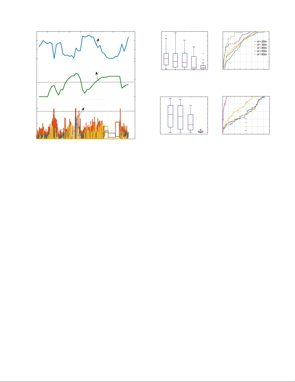
Loading high-quality paper...
Comments & Academic Discussion
Loading comments...
Leave a Comment