High Impedance Fault Detection and Isolation in Power Distribution Networks using Support Vector Machines

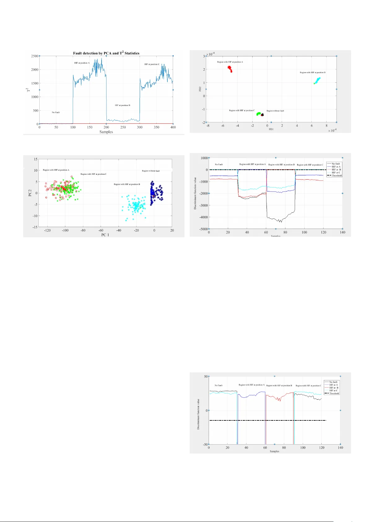
High Impedance Fault Detection and Isolation in Po wer Distrib ution Networks using Support V ector Machines Muhammad Sarwar ∗ , Faisal Mehmood, Muhammad Abid, Abdul Qayyum Khan, Sufi T abassum Gul, Adil Sarw ar Khan Department of Electrical Engineering, P akistan Institute of Engineering and Applied Sciences Islamabad, P akistan Abstract This paper proposes an accurate High Impedance Fault (HIF) detection and isolation scheme in a power distribution network. The proposed schemes utilize the data av ailable from voltage and current sensors. The technique employs multiple algorithms consisting of Principal Component Analysis, Fisher Discriminant Analysis, Binary and Multiclass Support V ector Machine for detection and identification of the high impedance fault. These data dri ven techniques hav e been tested on IEEE 13-node distribution network for detection and identification of high impedance faults with broken and unbroken conductor . Further , the robustness of machine learning techniques has also been analysed by examining their performance with variation in loads for di ff erent faults. Simulation results for di ff erent faults at v arious locations have sho wn that proposed methods are fast and accurate in diagnosing high impedance faults. Multiclass Support V ector Machine gi ves the best result to detect and locate High Impedance Fault accurately . It ensures reliability , security and dependability of the distrib ution network. K eywor ds: Fisher Discriminant Analysis, High Impedance Fault, Principal Component Analysis, Support V ector Machines 1. Introduction Detection of high impedance faults poses a highly challeng- ing problem because of the random, asymmetric and nonlin- ear nature of high impedance fault (HIF) current. Most of the time, these faults cannot be detected and isolated by conv en- tional over -current schemes, because magnitude of fault current is considerably lower than nominal load current ( Jones , 1996 ). High impedance faults typically occur when an ener gised conductor comes in contact with ground through any high impe- dance object such as dry asphalt, wet sand, dry grass and sod etc. which limits the flo w of current to wards ground ( Jones , 1996 ). T imely detection of high impedance faults is neces- sary for e ffi cient, reliable and safe operation of power systems. Probability of occurrence of high impedance fault in distribu- tion networks is more than in transmission network because dis- tribution feeders are more likely to come in contact with high impedance objects like trees etc. Howe ver , in underground ca- bles high impedance faults are caused by insulation de grada- tion that exposes the energised conductor to high impedance objects ( Bakar et al. , 2014 ). High impedance faults occur at voltage level of 15KV or belo w in most of the cases. Mag- nitude of HIF current is independent of the conv entional short circuit fault current le vel ( Bishop , 1985 ). High impedance faults are extremely di ffi cult to detect and isolate by con ventional protection schemes, because fault cur- rent magnitude is much lower than nominal current. According to report by Power System Relaying Committee (PSRC), only 17% of HIFs can be detected by con ventional relaying schemes ( Jones , 1996 ). Detection of HIFs helps in prognostic mainte- nance in po wer distribution system. High impedance faults in- volv e arcing which makes fault current asymmetric and nonlin- ear . As a result of arcing, HIFs inv olve high frequency com- ponents similar to load and capacitor switching which makes detection much more di ffi cult ( Sahoo and Baran , 2014 ). Previous research on diagnosis of HIFs was focused on lab- based staged f ault studies. Howe ver , with the adv ancement in technology and better understanding of features of HIFs, the focus has shifted to wards simulations and software studies ( Brahma , 2013 ). Due to its critical nature, researchers from both industry and academia hav e proposed various techniques to detect HIFs in distribution networks. Majority of the studies were reported as early as 1980s and 1990s, but the simulation methods and ad- vanced detection techniques are still being dev eloped and pro- posed. HIF detection methods can be broadly classified into time domain algorithms, frequency domain algorithms ( Lima et al. , 2018 ), hybrid algorithms ( Samantaray et al. , 2008 ) and knowledge-based systems ( Etemadi and Sanaye-P asand , 2008 ). K. Zoric and M. B. Djuric presented a method to detect high impedance f ault based on harmonic analysis of voltage signals ( Zoric et al. , 1997 ). James Stoupis introduced a new relaying scheme manufactured by ABB in the area of artificial neural networks ( Stoupis et al. , 2004 ). Sedighi proposed two methods based on soft computing for detection of HIF ( Sedighi et al. , 2005 ). Mark Adamiak proposed signature based high impedance fault diagnoses which in volves expert system pat- Pr eprint submitted to Journal of King Saud Univer sity - Engineering Sciences September 25, 2019 tern recognition on harmonic energy le vels in arcing current ( Adamiak et al. , 2006 ). S.R. Samantaray presented an intelligent approach to de- tect high impedance f aults in distribution systems ( Samantaray , 2012 ). In ( Zanjani et al. , 2012 ), authors hav e proposed a new approach to detect HIF based on PMU (Phasor Measurement Unit). F . V . Lopes presented a method to diagnose HIF in smart distribution systems ( Lopes et al. , 2013 ). Authors in ( Brahma , 2013 ; Hou , 2007 ) presented a method to detect HIF based on mathematical morphology . A new model for high impedance faults has been present in ( T orres et al. , 2014 ). Results of this model are quite closer to what is observed in staged faults. This research activity also detected HIF using harmonic analysis of current wa veform. Recenlty , Kavi presented a method to detect HIF in Single W ire Earth Return (SEWR) system ( Kavi et al. , 2016 ). Sekar and Mohanty proposed fuzzy rule base approach for high impe- dance fault detection in distribution systems ( Sekar and Mo- hanty , 2018 ). The y present a filter-based morphology gradient (MG) to di ff erentiate non-HIF e vents from HIF events. W . C. Santos presented a transient based approach to identify HIF in power distribution systems ( Santos et al. , 2017 ) . In ( Ferdo wsi et al. , 2017 ), real time complexity measurement (RCM) based approach is used to detect HIF . In ( Ghaderi et al. , 2016 ) HIF de- tection techniques are ev aluated and compared with each. W ith the advancement in technology , the trend has been shifted to- wards smart grids and smart distribution systems. Smart dis- tribution systems include measurements (such as voltage and current) at each node that helped to discover and develop digi- tal signal processing based fault detection techniques ( Lai et al. , 2005 ; Elkalashy et al. , 2007 ; Sheelv ant , 2015 ). Prior studies ha ve helped to re veal many of the hidden char- acteristics of High Impedance Faults. But the major drawback of aforementioned techniques is that the y are not capable of de- tecting all types of high impedance faults. Furthermore, active methods of HIF detection use signal injection which deterio- rates the power quality . Some methods employ data gathered by PMUs, which are quite expensiv e and also man y distribution systems currently don’t deploy PMUs. Another disadv antage is that most of the proposed methods use a lot of computing po wer and thus can not be implemented on an embedded system as a portable numerical relay . The motiv ation for this research work lies in manifold short- comings of the prior research. The proposed method is compu- tationally less rigorous, so it can be implemented on an embed- ded system as a numerical relay . The method ensures po wer quality as it does not inject any signal into power system for HIF detection. The technique de veloped can detect all types of HIF i.e., broken and unbroken conductor HIFs and can lo- cate the faulty section of network. Furthermore, input data is gathered using CTs and PTs which are already deployed in all distribution networks, so no additional hardware installation is needed for data acquisition. The proposed method is accurate and highly reliable as it can distinguish load switching from faults, and can also detect and isolate multiple high impedance faults in the power network. The training model used for de- tecting faults is of low order and can easily be implemented on any embedded hardware for real time prototyping and HIF detection. In proposed method, data obtained from voltage and cur- rent sensors is fed to three fault detection algorithms i.e., Prin- cipal Components Analysis (PCA), Fischer Discriminant Anal- ysis (FDA) and Support V ector Machines (SVM). PCA extracts principal components of data and use them for fault detection. FD A reduces the data to a lower dimension to maximise dis- tance among various classes for increased accurac y . Binary class SVM is used only for detection of HIFs. T o determine type and location of f ault multiclass SVM is deployed to signal the presence of an incipient or sudden high impedance fault. Once the fault is detected, the faulty system can be isolated from the network by issuing a trip signal to traditional ov er cur - rent relays in substation. The speed and accuracy of proposed method is comparable to con ventional fault detection of ov er- current faults. The rest of research paper is organised as follows. Sec- tion II details characteristics and features of high impedance faults. Theoretical foundation for data driven techniques is laid down in Section III. Proposed techniques have been tested on IEEE 13-node test system and results are discussed in Section IV . Section V concludes the research. 2. High Impedance Fault Characteristics In this section, prominent features of high impedance faults are described. T o obtain training data from simulation, a fault model is simulated in Simulink and training data is obtained from voltage and current sensors installed in the netw ork. 2.1. Pr operties of High Impedance F aults Arcing is a prominent phenomena in HIFs. The arc is formed due to air gap between energised conductor and high impedance object. Arc ignition occurs when magnitude of voltage is higher than air gap breakdown voltage. Consequently , arc extinction occurs when v oltage is lo wer than breakdown v oltage ( Ghaderi et al. , 2016 ). The value of break do wn voltage changes during each cycle. Thus, in e very c ycle of voltage, the HIF current includes two arc re-ignitions and two arc extinctions. There- fore, current conducting path changes during each cycle which changes the magnitude of HIF current making it non-linear , also HIF current is intermittent in nature ( Ghaderi et al. , 2016 ). Some of the typical features of high impedance faults are as follows: • Non linearity: V oltage-current characteristics are highly nonlinear due to change in current conducting path ( Chen et al. , 2013 ). • Asymmetric nature of HIF current: Peak values of cur- rent are di ff erent in positiv e and negati ve half cycle due to the presence of v arying break down voltage ( Ghaderi et al. , 2016 ; Biswal , 2017 ). • Intermittent natur e: HIF current is not steady due to intermittent nature of arc ( Mai et al. , 2012 ). 2 Fig. 1: The selected HIF model ( Brahma , 2013 ) • Build up: Current magnitude progressi vely increases till it reaches it maximum value ( Bisw al , 2017 ) • Randomness: Magnitude of HIF current and its shape changes with time due change in impedance of conduct- ing path ( Sykulski , 2006 ). • Low and high frequency components: HIF current in- cludes low frequency components due to non-linearity of HIF . Additionally , HIF current also contains high fre- quency components due to intermittent nature of arc ( Ghaderi et al. , 2016 ). 2.2. Simulation of High Impedance F ault T o obtain training data from simulation, appropriate model of HIF is required which w ould sho w real behaviour of an HIF . This paper utilises an HIF model sho wn in Fig. 1 , connected between any of phase and ground ( Brahma , 2013 ). The model is simulated in MA TLAB, the parameters of model are tuned according to test feeder . In this HIF model, two diodes D p and D n are connected to two DC v oltage sources V p and V n , respectiv ely . The DC sources have di ff erent magnitude and their magnitude randomly changes around V p and V n after e very 0.11 ms. This models the asymmetric nature of arc current and intermediate arc extinc- tion. T o model the randomness in duration of arc e xtinction in high impedance fault, voltage polarity also changes at every sampling instant ( Brahma , 2013 ). When the instantaneous value of phase voltage is greater than V p , current flows to wards ground, when the instantaneous value of phase voltage is less than V n , current reserves its direction, when the instantaneous value of phase voltage is between V p , and V n , no current flows. In order to incorporate varying arc resistance, the model of HIF also in- cludes two variable resistances, R p and R n , such that values of these resistances vary randomly after e very 0.11 ms. The parameters used for HIF model with IEEE 13-node test feeder in Simulink are: Fig. 2: Arc current and voltage during HIF Fig. 3: The v-i characteristics of HIF V p = 1 . 0 kv , wit h ± 10% var iat ion V n = 0 . 5 kv , wit h ± 10% var iat ion R p , R n = 1000 Ω − 1500 Ω , wit h rand om var iation The abov e model is simulated in Matlab R  . There are two steps in volv ed in modelling HIF; in first step, v ariable DC v olt- age sources are modelled using controlled voltages source; in second step, variable resistances are modelled using controlled current sources. First part is implemented using only random number generator , constant block, and controlled voltage source is used to obtain v arying DC voltages. Second step in volv es a b uild-up series R-L circuit and a sinusoidal signal of 60 Hz. Both of these generate an exponentially growing sine wav e. The sine wa ve is multiplied with a random number of amplitude 1 and variance of 0.12 to obtain a randomly v arying resistance. Fig. 2 shows arc current and voltage wa veforms obtained as a result of modelling HIF in Simulink, using HIF model of Fig. 1 . It is clear that the arc current is small, random, asym- metric, and nonlinear in nature. The voltage wav eform in Fig. 2 3 also shows the random behaviour . Fig. 3 shows the v-i char- acteristics of HIF , the v-i characteristics of HIF and the cur - rent wa veform are quite similar to those got from a staged fault ( Brahma , 2013 ). 3. Theoretical F oundation Data driven techniques are the perfect candidate for fault diagnoses in large systems where enough amount of data is av ailable. Principal Component Analysis, Fischer Discrimi- nant Analysis, and Support V ector Machines are widely used for addressing diagnosis problems due to their simplicity and e ffi ciency in processing large amount of data. Here the theoret- ical basis for applied algorithms is giv en. 3.1. Principal Component Analysis Principal Component analysis is linear dimensional reduc- tion technique, it projects higher dimensional data into lower dimensions while keeping significant features. PCA has ability to retain maximum variation that is possible in lo wer dimen- sions such that transformed features are linear combination of primary features. In reduced dimensions, di ff erent statistical plots such as T 2 or Q-charts are utilised for visualisation of dif- ferent trends. PCA is known as po werful tool for feature e xtrac- tion and data reduction in f ault detection techniques because of simplicity and its ability to process large amount of data ( Jamil et al. , 2015 ). Application of PCA for fault diagnoses consists of three steps; first of all, loading vectors (transformation vectors) are calculated by performing o ffl ine computations on training data; in second step, the loading vectors are utilised to transform on- line data (higher dimensional data) into lower dimensions; in third step, test statistics such as T 2 are used to detect fault ( Jamil et al. , 2015 ). Let us assume that a training set of m process v ariables, with set of n observations, is normalised to unit variance and zero mean by subtracting each process variable by its mean and di- viding by standard deviation of data, and is shown in the form of input matrix X ∈ R n × m . W ith the help of singular value decompo- sition of input data matrix X, loading vectors or transformation vectors are calculated. 1 √ 1 − n X = U Σ V T (1) In equation ( 1 ), U and V are unitary matrices, and Σ is called diagonal matrix and its singular values are in decreasing order . The transformation vectors are orthonormal vectors of matrix V ∈ R m × m . Training set’ s variance projected along the u th col- umn of V is equal to σ 2 u . In PCA, loading vectors or trans- formation vectors related to a largest singular value are kept to capture large data v ariation in lower dimensions. Let us assume that P ∈ R m × a is the matrix with first a column of V ∈ R m × m , and projection of observed data X into reduced dimensions are incorporated in the score matrix T is giv en as, T = X P (2) Fig. 4: Flowchart for o ffl ine f ault computation using PCA Once the data is projected in lower dimensions, Hotteling’ s T 2 statistics is used for fault detection. Hotteling’ s T 2 - statistics can be calculated as ( Jamil et al. , 2015 ; Chiang et al. , 2000 ), T 2 = x T P Σ − 1 a P T x (3) where Σ is the diagonal matrix of first a singular v alues, P is the loading vector matrix corresponding to first a singular val- ues. The Hotteling’ s T 2 - statistics ( 3 ) is scaled squared 2-norm of observation space X, measures systematic variations of the process, and if there is violations, it will indicate that system- atic variations are out of control. If α is the level of significance, the threshold of T 2 statistics can be calculated as ( Chiang et al. , 2000 ), T 2 α = m ( n − 1)( n + 1) n ( n − m ) F α ( m , n − m ) (4) Where F α ( m , n − m ) is known as F-distribution with m and (n- m) de gree of freedom ( Chiang et al. , 2000 ). Essential condition for fault detection occurs if Hotteling’ s T 2 - statistics exceeds its threshold value, that is, T 2 ≤ T 2 α F ault f ree ca se T 2 > T 2 α sF ault ca se A complete flowchart for o ffl ine and online computation of the PCA algorithm for fault detection is shown in Fig. 4 and 5 , respectiv ely . 3.2. F isher discriminant analysis Fisher discriminant analysis is one of the most powerful methods for dimensionality reduction. In case of fault detec- tion, PCA gi ves very good results. Howe ver , it has poor prop- erties of fault classification because it does not consider infor- mation (variance) among di ff erent classes of data during com- putation of loading vectors ( Jamil et al. , 2015 ). FD A consid- ers information among di ff erent classes of data, so it is more fa vourable for fault classification. It determines a set of trans- formation vectors, known as FD A vectors. FD A v ectors max- imise the information (distance) among di ff erent classes of data, 4 Fig. 5: Flowchart for online f ault computation using PCA while minimising information within each class in projected space. FD A tries to centralise di ff erent data classes and fea- ture recognition rates of FDA is better than PCA. According to ( Adil et al. , 2016 ), performance of FD A for fault detection and classification is quite better than that of PCA. The procedure to implement FDA is similar to PCA. First of all, FD A v ectors are computed using training data, then these FD A vectors are utilised to transform online data into lower di- mensional space. Finally , a discriminant function isolates the fault. In FDA training data, both normal and faulty data is used for computation of FDA vectors, howe ver , in PCA only nor- mal data is used for computation of loading v ectors ( Adil et al. , 2016 ; Chiang et al. , 2000 ). In order to detect f ault with the help of FD A, Hotteling’ s T 2 - statistics is used. Let us assume that a training set of m process variables, with set of n observations, is sho wn in the form of input matrix X ∈ R n × m . Consider q as number of classes in di ff erent faults and n k is number of observations in k t h class, let x i be the transpose of i th row of matrix X. The transformation v ector ν is computed using training data such that following optimisation is solv ed. J F D A ( ν ) = arg ma x ν , 0 ν T S b ν ν T S w ν (5) Where S w shows within class scatter matrix gi ven by S w = Σ q k = 1 S k (6) W ith S k = Σ n x i ∈ χ k ( x i − x k )( x i − x k ) T (7) and the mean of kth class x k = 1 n k Σ x i ∈ x k x i similarly S b is be- tween class scatter matrix giv en by S b = Σ q 1 ( x i − x k )( x i − x k ) T (8) W ith x shows the combined (total) mean vector given by x = 1 n Σ n i = 1 x i it is stated that solution to abov e optimisation problem is identical to eigen value decomposition problem ( Ding , 2014 ), S b ν h = λ h S w ν h (9) Where λ h is generalised eigenv alue representing the extent of separability between classes and λ h are respective eigen vec- tors. Equation ( 5 ) shows optimisation problem that ensures minimum scatter within class and maximum scatter between di ff erent data classes. This feature helps to classify faults. In order to project online data into lo wer dimensional space, a ma- trix V q ∈ R ( m × q − 1) with q-1 FD A v ectors is defined as, such data projected data z i ∈ R ( q − 1) is giv en by z i = V T q x i (10) For fault detection Hotteling’ s T 2 - statistics is used ( Y in et al. , 2012 ), giv en by T 2 k = x T V a ( V T a S k V a ) − 1 V T a x (11) Where a shows the number of non-zero eigenv alues. For a giv en lev el of significance α , threshold for Hotteling’ s T 2 - statistics is giv en by: T 2 α = a ( n − 1)( n + 1) n ( n − 1) F α ( a , n − a ) (12) T 2 k ≤ T 2 α F ault f ree ca se T 2 > T 2 α F ault ca se For fault classification, the discriminant function is used as given below: g k ( x ) = − 1 2 ( x − x k ) T V q ( 1 n k − 1 V T q S k V q ) − 1 V T q ( x − x k ) + ln ( q i ) − 1 2 ln [ d et ( 1 n k − 1 V T q S k V q )] (13) In abov e equation, g k (x) is the discriminant function associ- ated with class k, provided a data vector x ∈ R m , online data is associated with class i provided that the discriminant function belonging to i t h class is maximum for a fault in class i , can be expressed as, g i ( x ) > g k ( x ) (14) A complete flowchart for o ffl ine training of the FDA algorithm is shown in Fig. 6 . 3.3. Support V ector Machines (SVM) SVM is a well-known data driv en technique used for detec- tion and classification of faults due to its generalisation abil- ity and being less susceptible to the curse of dimensionality ( Burges , 1997 ). For the first time, Support vector machines were used by V apnik ( Zhang , 2010 ). It is one of the new ma- chine learning tools for classification of linear and nonlinear data. SVM is a binary classifier that maximises the margin be- tween two data classes through a hyper-plane as shown in Fig. 7 . SVMs maximise the mar gin near separating hyperplane. The decision of separation is fully identified by the support vectors. Solution of SVM is obtained through solution of quadratic pro- gramming. In SVM, a discriminant function is used to di ff erentiate dif- ferent classes of data giv en by: f ( x ) = w T x + b (15) 5 Fig. 6: Flowchart for o ffl ine training of FD A Where b, the bias, x, the data points, and w , the weighting vector , are obtained through training data. In two-dimensional space, the discriminant function is a line, in three-dimensional space, the discriminant function is a plane, and in n-dimensional space, the discriminant function is a hyperplane. SVM gener- ates the optimal separating hyperplane by calculating the value of bias, weighting vector in such way that maximum mar gin is achiev ed. The points in training set with least perpendicular distance to the hyperplane are known as support vectors. The margin of the optimal separator can be defined as width of sep- aration between support vectors. ρ = 2 f ( x 0 ) w = 2 r (16) 3.3.1. The K ernel T rick (F eature Space) The cases in which training data is not linearly separable in the original space using above methods, then, this kind of data can be mapped to a higher-dimensional space which makes the data separable ( Nayak , 1998 ), as shown in Fig. 8 . A kernel function is a type of function that corresponds to an inner product in the higher dimensional space. For e xample, if data is mapped to feature space through a transformation Φ : x → ϕ ( x ), then, the inner product results: K ( xi , x j ) = φ ( x i ) T φ ( x j ) (17) There are di ff erent types of kernels, such as, polynomial, linear , Radial Basis Function (RBF) etc. The discriminant function of SVM, can be written as: f ( x ) = w T x + b (18) Fig. 7: Linear separating hyperplane ( Nayak , 1998 ) Fig. 8: Mapping of data to feature space ( Nayak , 1998 ) According to Representer theorem, w can be written as linear combination of input vectors. w = Σ N j = 1 α j x j (19) Thus f ( x ) = w T x + b = b + Σ N l = 1 α l x T l x (20) All the dot products can be replaced with k ( c , d ) = c T d (21) Optimisation problem: min a , b 1 2 Σ N j , l = 1 α j α l k ( x j , x k ) + C Σ N j = 1 ξ j (22) Where ξ j > 0 y j Σ N l = 1 α l k ( x l , x j ) + b ≥ 1 − ξ j (23) In order to test the pattern, we use: f ( x ) = b + Σ N l = 1 α l k ( x l , x ) (24) Euclidean dot product can be substituted with dot product in feature space “ Φ ”, which will permit nonlinear classification. k ( c , d ) = Φ ( c ) T Φ ( d ) (25) k ( c , d ) is kno wn as kernel function and corresponding SVM is called kernelized SVM. This type of SVM can solve the issue of classification of not linear separable data. Steps in volved in implementation of kernelized SVM are: 6 Fig. 9: IEEE 13-node Distribution T est Feeder Step 1: Input data is normalised. Step 2: T raining of SVM. Step 2.1: Selection of kernel function. Step 2.2: Selection of kernel parameter . Step 2.3: Optimisation of penalty factor (C). Step 2.4: Cross validation. Step 3: Classification of SVM test data. 3.3.2. Multiclass SVM Binary class SVM can be used for fault detection, b ut it can- not be used for fault classification. Ho we ver in practical cases, discrimination of more than two classes is required, hence, mul- ticlass pattern recognition is often required in real world prob- lems ( Xue , 2014 ). In majority of cases, multiclass pattern recog- nition problems are decomposed into series of binary problems such that binary pattern recognition techniques can easily be applied in practical cases. multiclass SVM algorithms such as one-versus-one, one-versus-all, can be applied be applied to classify more than two faults. 4. Application of Data Dri ven T echniques to Diagnose HIF HIF is introduced at di ff erent positions and di ff erent phase conductors of IEEE 13-node test feeder as shown in Fig. 9 . In data structure, data is generated from Simulink model of test feeder . There are 29 variables of singles phase, two phase and three phase voltages of 13-node test feeder . Data has been placed in input matrix in such a way that each column of in- put matrix represents v oltage and each ro w of input matrix rep- resents number of observations. There were 400 observations recorded for bus voltages, first 100 observations correspond to normal data, while other 300 observations correspond to three HIF locations at di ff erent positions of test feeder . 4.1. Detection of HIF using PCA and Hotteling’ s T 2 statistics For diagnoses of HIF using PCA, training data consisting of 60 samples of normal condition (without fault) has been se- lected while testing data is consist of 100 samples of non-f aulty Fig. 10: Projection of training data and testing in two dimensional space for PCA Fig. 11: The results of Hotteling’ s T 2 statistics to detect HIF data and 100 samples of faulty data. PCA algorithm has been applied on training data and 29 principal components are ob- tained. Out of 29 principal components only 5 principal com- ponents have been retained, the decision is made on the basis of total variance captured by these 5 principal components. The value of α , as mentioned in ( 4 ), is taken 0.001. As we have retained 5 principal components so ( 1 . 6983 1 . 72 ) = 98% of total v ari- ance has been captured by first fiv e principal components. Fig. 10 shows projection of training data and testing in two dimensional space. It can be observed that first two components capture most of variation in higher dimensional data. Fig. 11 shows the results of Hotteling’ s T 2 statistics to detect HIF after applying (3.3) on test data. It can be seen that normal data (first 100 samples) lies belo w threshold value of T 2 statistics, where threshold value is 22.0108. This threshold value was found using significance lev el of 0.1% and confidence region of 99%. PCA can successfully detect high impedance fault as sho wn in Fig. 11 . In some cases, it is required to classify di ff erent types of HIFs such as broken conductor and unbroken con- ductor HIFs at di ff erent locations of feeder . For this purpose, High impedance faults at three di ff erent locations are analysed. Fig. 12 sho ws plot of Hotteling’ s T 2 statistics to detect HIFs at three di ff erent locations. Results show that PCA can suc- cessfully detect these three HIFs. Only 5 principal components are retained such that (1.6983 / 1.72) = 98% of total variance has been captured. Fig. 13 shows projection of training data and test 7 Fig. 12: Plot of Hotteling’ s T 2 statistics to detect multiple HIFs Fig. 13: Projection of training and test data in 2-D space for multiple faults data in two dimensional space, it can be seen that PCA cannot discriminate between di ff erent types of HIFs, this is due to the reason that PCA do not consider information among di ff erent classes of data. W e can conclude that PCA is suitable for HIF detection but it cannot classify di ff erent types of HIFs. 4.2. Detection of HIF using FD A FD A is applied for detection and isolation of high impedance faults in power distribution systems. In order to compute FD A vectors, both normal and faulty data is used, in this work, 60 samples in training data and 40 samples in test data correspond- ing to each scenario, that is, faulty and non-faulty case. Fig. 14 shows projection of training data in two-dimensional space by FD A. In second step, after computation of transformation vec- tors (FD A vectors), the discriminant function is used to test on- line data. Fig. 15 shows plot of discriminant function in each category . It can be observed that up to first 30 samples, v alue of discriminant function corresponding to normal case has max- imum magnitude, which shows that there is no fault in test feeder . Similarly , after 30 samples, value of discriminant func- tion corresponding to fault at position A has maximum magni- tude, which sho ws that fault at position has occurred. Same is the case with fault at position B and C. Zoomed vie w of plot is shown in Fig. 16 . The abo ve results hav e shown that FD A can successfully isolate / locate HIF . This technique is very well suited for moni- toring of power distrib ution systems. Fig. 14: Projection of training data in two dimensional space by FD A Fig. 15: Plot of discriminant function for multiple HIF detection using FD A 4.3. Detection of HIF using SVM Support vector machine algorithm has been applied for 29- dimensional data without any dimensional reduction technique. Selection of optimal value of penalty factor is important, this is done by performing nested 3-fold cross v alidation in original data. W ith the help of cross validation, av erage area under the curve was computed for 1000 values of penalty factor between 0.1 and 100. After selection of optimal v alue of C, SVM classi- fiers were trained with optimal penalty factor and validated on training data so that generalisation would be checked. T est data of HIF was classified by validated SVM classifier . The pre- dicted labels of test data fairly detects the occurrence of fault, that is -1 for non-faulty data and + 1 for faulty data as shown in Fig. 16: Zoomed view of discriminant function for multiple HIF detection using FD A 8 Fig. 17: Classification of an HIF using binary-class SVM Fig. 17 . 4.4. Detection and Classification of HIF using M-SVM Binary class SVM can be used for fault detection, but it cannot be used for fault classification. Howe ver , in Power dis- tribution systems, discrimination of more than two classes is re- quired, hence, multiclass pattern recognition is often required in monitoring Power distrib ution systems. Multiclass SVM (M– SVM) classifier is obtained using training of non-fault cases with class label 4, fault at position A with class label 3, fault at position B with class 2, and fault at position C with class 1. In each classifier , during training, a Gaussian Radial Basis Function kernel with a scaling factor , sigma ( σ ), of 0.5 and a penalty factor of 10 is used. The tolerance value for Karush- Kuhn-T ucker (KKT) condition for the training of data is taken as 0.001. The v alue of regularization parameter , lambda ( λ ) is 1. T est data is classified using the trained classifiers for 50 observations of each data class and predicted labels were di ff er- entiated with known data labels. Fig. 18 shows that up to 50 samples, the predicted labels belong to normal class data, indicating that there is no fault. After first 50 samples, predicted labels belong to class label 3, indicating that the fault is occurred at position A. After first 100 samples, predicted labels belong to class label 2, indicating that the fault is occurred at position B. similarly , after first 150 samples, predicted labels belong to class label 1, indicating that the fault is occurred at position C. Similarly , Fig. 19 show the score plot of test data for each class of data. A comparison is presented to ev aluate the results of the proposed technique with those from literature and observ ations hav e been recorded in T able 1 . After testing the technique on 400 test cases, it is found that proposed method is extremely quick and e ffi cient in detecting HIFs. The proposed method is ev aluated through the following performance indices: Dependability: Predicted HIF cases / Actual HIF cases. Security: Predicted non-HIF cases / Actual non-HIF cases. T able 1 compares the performance indices of the proposed method. It is noted that the proposed method detects all HIF faults under various operating conditions and disturbances. Thus, the proposed method is accurate, reliable and prompt in the de- tection of High Impedance Faults. Fig. 18: Predicted labels of test data using Multiclass–SVM classifier Fig. 19: Predicted labels of test data using M–SVM classifier on a 2-D plane It can be seen that M-SVM can easily classify high impedance faults at di ff erent locations with load variation and capacitor switching. So, we can conclude that SVM based techniques can successfully detect and locate HIFs in a Po wer Distribution Network. 5. Conclusion In this research paper , high impedance fault detection and classification in po wer distribution systems has been studied us- ing data driv en techniques. Source-diode-resistance model con- sisting of two diodes with opposite polarity connected to DC sources is utilised to simulate the high impedance fault. Data driv en techniques including PCA, FDA, and SVM are applied to detect / classify HIFs. PCA along with Hotteling’ s T 2 statis- tics to detect HIFs, it is demonstrated that PCA successfully detects HIF but it cannot classify HIFs. Compared to that, FD A can also successfully classify / locate the fault. Further supe- rior results are achieved by M-SVM, fault classification rate of SVM is better than FD A. M-SVM algorithm can detect all types of HIF and is also robust against capacitor and load switching transients in distribution netw ork. Conflict of Interest The authors declare no conflict of interest. 9 T able 1: Comparison of performance indices of the proposed M-SVM method with previous techniques Method Security (%) Dependability (%) W av elet transform ( Chen et al. , 2016 ) 68.5 72 T ime frequency transform Samantaray et al. ( 2008 ) 81.5 98.3 Morphological gradient ( Sarlak and Shahrtash , 2011 ) 96.3 98.3 Mathematical Morphology ( Gautam and Brahma , 2012 ) 100 100 The proposed method (M-SVM) 100 100 References Adamiak, M., W ester , C., Thakur , M., Jensen, C., 2006. High impedance fault detection on distribution feeders. GE Industrial solutions . Adil, M., Abid, M., Khan, A.Q., 2016. Comparison of PCA and FDA for monitoring of coupled liquid tank system,. Pakistan. Bakar , A.H.A., Ali, M.S., T an, C., Mokhlis, H., Arof, H., Illias, H.A., 2014. High impedance fault location in 11 kv underground distribution systems using wa velet transforms,. Electrical Power and Ener gy Systems 55, 723– 730. Bishop, R.E.L.M.T ., 1985. A comparison of measured high impedance fault data to digital computer modeling results,. IEEE Transactions on Power Apparatus and Systems 104, 2754–2758. Biswal, A.P .K.T ., 2017. Detection of high impedance fault in distrib ution sys- tem considering distributed generation,. Bangalore, India. Brahma, S.G.S.M., 2013. Detection of high impedance fault in power distri- bution systems using mathematical morphology ,. IEEE TRANSA CTIONS ON PO WER SYSTEMS 28, 1226–1234. Burges, C.J.C., 1997. A T utorial on Support V ector Machines for Pattern Recognition,. Kluwer Academic Boston. Chen, J., Phung, T ., Blackburn, T ., Ambikairajah, E., Zhang, D., 2016. De- tection of high impedance faults using current transformers for sensing and identification based on features extracted using w av elet transform. IET gen- eration, transmission & distribution 10, 2990–2998. Chen, J.C., Phung, B.T ., Zhang, D.M., Blackbur , T ., 2013. Study on High Impedance Fault Arcing Current Characteristics,. T AS, AustraliA, Hobart. Chiang, L., Russel, E., Braatz, R., 2000. Advanced T extbooks in Control and Signal Processing. Springer New Y ork. Ding, S.X., 2014. Data-driven Design of Fault Diagnosis and Fault-tolerant Control Systems. Duisburg,German y: Springer. Elkalashy , N.I., Lehtonen, M., Darwish, H.A., 2007. A novel selectivity tech- nique for high impedance arcing fault detection in compensated mv net- works,. EUROPEAN TRANSA CTIONS ON ELECTRICAL POWER 18, 344–363. Etemadi, A., Sanaye-Pasand, M., 2008. High-impedance fault detection using multi-resolution signal decomposition and adapti ve neural fuzzy inference system. IET generation, transmission & distribution 2, 110–118. Ferdowsi, F ., V ahedi, H., Edrington, C.S., 2017. High impedance fault detection utilizing real-time complexity measurement,. TX, USA. Gautam, S., Brahma, S.M., 2012. Detection of high impedance fault in power distribution systems using mathematical morphology . IEEE Transactions on Power Systems 28, 1226–1234. Ghaderi, A., Ginn, H.L., Mohammadpour, H.A., 2016. High impedance fault detection: A revie w ,. Electric Power Systems Research 143, 376–388. Hou, D., 2007. Detection of High-Impedance Faults in Power Distribution Systems,. Jamil, F ., Abid, M., Haq, I., Khan, Q.A., Iqbal, M., 2015. Fault diagnosis of pakistan research reactor-2 with data-dri ven techniques,. Annals of Nuclear Energy 90, 433–440. Jones, B.M.A.R.H., 1996. High impedance f ault detection implementation is- sues,. IEEE 11, 139. Kavi, M., Mishra, Y ., V ilathgamuwa, D.M., 2016. Detection and identification of high impedance faults in single wire earth return distribution networks,. QLD, Australia, Brisbane. Lai, T .M., Snider , L.A., Lo, E., Sutanto, D., 2005. High-impedance fault detec- tion using discrete wa velet transform and frequency range and rms conv er- sion,. IEEE TRANSACTIONS ON PO WER DELIVER Y 20, 397–407. Lima, ´ E.M., dos Santos Junqueira, C.M., Brito, N.S.D., de Souza, B.A., de Almeida Coelho, R., de Medeiros, H.G.M.S., 2018. High impedance fault detection method based on the short-time fourier transform. IET Gen- eration, T ransmission & Distribution 12, 2577–2584. Lopes, F .V ., Santos, W .C., Fernandes, D., Ne ves, W .L., 2013. A transient based approach to diagnose high impedance f aults on smart distribution networks. Mai, W ., Phung, B.T ., Ambikairajah, E., 2012. Detection of high impedance faults in medium voltage distrib ution networks,. V ietnam. Nayak, C.M.P ., 1998. Support vector machines and machine learning on docu- ments,. In Introduction to information Retriev al. Sahoo, S., Baran, M.E., 2014. A method to detect high impedance faults in distribution feeders, in: 2014 IEEE PES T&D Conference and Exposition, IEEE. pp. 1–6. Samantaray , S., Panigrahi, B., Dash, P ., 2008. High impedance fault detection in po wer distrib ution networks using time–frequency transform and proba- bilistic neural network. IET generation, transmission & distribution 2, 261– 270. Samantaray , S.R., 2012. Ensemble decision trees for high impedance fault de- tection in po wer distrib ution network,. Electrical Po wer and Energy Systems 43, 1048–1055. Santos, W .C., Lopes, F .V ., Brito, N.S.D., 2017. High-impedance fault iden- tification on distribution networks,. IEEE TRANSA CTIONS ON POWER DELIVER Y 32, 23–32. Sarlak, M., Shahrtash, S., 2011. High impedance fault detection using combi- nation of multi-layer perceptron neural networks based on multi-resolution morphological gradient features of current wav eform. IET generation, trans- mission & distribution 5, 588–595. Sedighi, A.R., Haghifam, M.R., Malik, O.P ., 2005. Soft computing applications in high impedance fault detection in distribution systems,. Electric Power Systems Research 76, 136–144. Sekar , K., Mohanty , N.K., 2018. A fuzzy rule base approach for high impedance fault detection in distribution system using morphology gradi- ent filter . Journal of King Saud University-Engineering Sciences . Sheelvant, B.P .P .V .R., 2015. High-impedance fault detection using wav elet transform,. International Journal of Engineering Research and General Sci- ence 3, 166–172. Stoupis, J., Maharsi, M., Nuqui, R., 2004. Ground alert: Reliable detection of high-impedance fault caused by do wned conductor . ABB Review , Jan . Sykulski, N.Z.J.K., 2006. Modelling arcing high impedances faults in relation to the physical processes in the electric arc,, Lisbon, Portugal. T orres, V ., Guardado, J.L., Ruiz, H.F ., Maximov , S., 2014. Modeling and de- tection of high impedance faults,. Electrical Power and Ener gy Systems 61, 163–172. Xue, Z.W .X., 2014. Multi-Class Support V ector Machine in Support V ector Machines Applications. Springer . Y in, S., Ding, S.X., Haghani, A., Hao, H., Zhang, P ., 2012. A comparison study of basic data-driv en fault diagnosis and process monitoring methods on the benchmark tennessee eastman process. Journal of Process Control 22, 1567–1581. Zanjani, M.G.M., Kargar , K.H., Zanjani, M.G.M., 2012. High impedance fault detection of distribution network by phasor measurement units,, T ehran, Iran. pp. 2–3. Zhang, Y .Z.Y ., 2010. A New Multi-class Classification Algorithm of Support V ector Machine,. Guangzhou, China. Zoric, K.J., Djuric, M.B., V , V ., 1997. Arcing faults detection on overhead lines from the voltage signals. International Journal of Electrical Power & Energy Systems 19, 299–303. 10