A Layered Architecture for Active Perception: Image Classification using Deep Reinforcement Learning

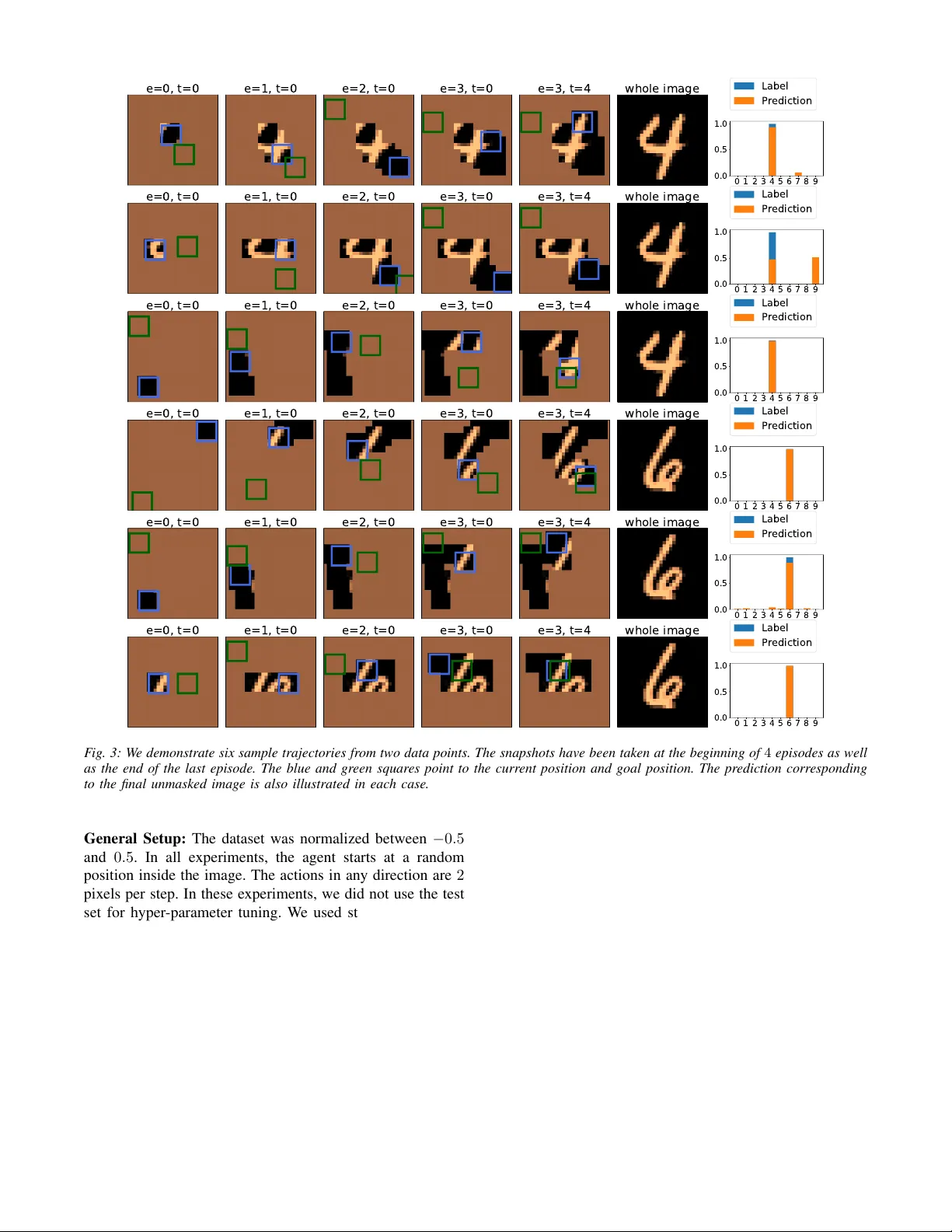
A Layer ed Ar chitecture f or Activ e P erception: Image Classification using Deep Reinf orcement Lear ning Hossein K. Mousavi, Guangyi Liu, W eihang Y uan, Martin T ak ´ a ˘ c, H ´ ector Mu ˜ noz-A vila, and Nader Motee 1 Abstract — W e propose a planning and perception mechanism for a robot (agent), that can only observe the underlying en vironment partially , in order to solve an image classification problem. A three-layer architecture is suggested that consists of a meta-layer that decides the intermediate goals, an action-layer that selects local actions as the agent navigates towards a goal, and a classification-layer that evaluates the reward and makes a prediction. W e design and implement these layers using deep reinf orcement learning . A generalized policy gradient algorithm is utilized to learn the parameters of these layers to maximize the expected reward. Our proposed methodology is tested on the MNIST dataset of handwritten digits, which pr ovides us with a level of explainability while inter preting the agent’ s intermediate goals and course of action. I . I N T RO D U C T I O N There has been a rapidly growing interest in goal rea- soning in recent years; planning mechanisms for agents that are capable of explicitly reasoning about their goals and changing them whenev er it becomes necessary [1], [2]. The potential applications of goal reasoning spans o ver sev eral research fields, for example, only to name a few , controlling underwater unmanned v ehicles [3], playing digital games [4], and air combat simulations [5]. One of the promising recent frame works for goal-based planning and reasoning is hierarchical deep Q-networks (hDQN) [6], which consists of two layers: a meta-layer that plans strate gically and an action-layer that plans local navigation. The meta-layer recei ves a state as its input and outputs a goal, a condition that can be e valuated in a giv en state. The action-layer receives a state and a goal as its input. Then, it selects and executes actions until the agent reaches a state where the goal is achiev ed. Both layers use a deep neural network similar to that of DQN with some important differences: the meta-layer selects goals in order to maximize external rewards from the en vironment, while the action- layer selects actions to maximize designer-defined intrinsic rew ards (e.g., 1 for reaching the goal state and 0 otherwise). In this work, we consider the problem of exploring an en vironment by a robot for classification purposes. Contrary to the standard assumptions made in the literature, we assume that robot can only partially observe the en vironment, where each observation depends on the actions taken by the robot. The first and second layers of our proposed architecture are 1 H.K.M., G.L., and N.M. are with the Department of Mechanical Engineering and Mechanics, Lehigh University , Bethlehem, P A 18015, USA { mousavi,gul316, motee } @lehigh.edu . W .Y . and H.M. are with the Department of Computer Science and Engineering, Lehigh Univ ersity { hem4, wey218 } @lehigh.edu . M.T . is with the Department of Industrial and Systems Engineering, Lehigh University { takac.mt } @gmail.com . similar to those of hDQN, while the third layer perform a classification task and ev aluates the reward in a differentiable manner . Our approach has other differences from hDQN. First, note that in hDQN requirement, the action-layer reaches a state achieving the goal. Ho wev er , find that this assumption is too restrictiv e, unnecessary , and potentially unrealizable due to partial observability for our purposes. Instead, our method relaxes this requirement by allowing a robot to mov e a few steps tow ards the goal, but not necessarily reaching to it. This fle xibility is needed because our intrinsic objecti ve is to explore the en vironment. Therefore, the goal planner should only dictate a desired general direction of exploration rather than imposing a hard constraint to reach a specific position. In this sense, our goals play a similar role to tasks in hierarchical task network planning [10], where the tasks are processes inferred from the agent’ s execution (e.g., “explore in this direction”) rather than goals, which need to be validated in a particular state (e.g., “reach coordinate (3 , 5) ”). Second, the nature of our problem motiv ates a single unified reward for the meta-layer and action-layer rather than separate rew ards. As already mentioned, this rew ard is the output of the classification layer . Lastly , the partial observability of our problem motiv ates deriv ation and use of policy-gradient approaches for learning the model parameters. As illustrated in [11], such generalized policy gradient algorithms allow co-design of goal generator , action planner , and classifier modules. Our methodology incorporates goal reasoning capabili- ties with deep reinforcement learning procedures for robot navigation by introducing intermediate goals, instead of requiring the robot to take a sequence of actions. In this way , our architecture provides transparency in terms of what the robot is trying to accomplish and, thereby , provides an explanation for its o wn course of action. The statement of the classification problem is identical to that of [11], but with some important dif ferences. In [11], we employ multiple agents with a recurrent network architecture, while robots do not enjoy goal reasoning capabilities. Related Literatur e: W e cast the classification problem as a planning and perception mechanism with a three-layer architecture that is realized through a feedback loop. W e are particularly interested in planning for perception. A related line of research is active perception: how to design a control architecture that learns to complete a task and at the same time, to focus its attention to collect necessary observations from the en vironment (see [12], [13] and references therein). The coupling between action and perception has been also e=0, t=0 e=1, t=0 e=2, t=0 c channels d 2 2 Conv. + ReLU d+c channels 2 2 MaxPool d+c channels 3d+c channels 2 2 MaxPool 2d 2 2 Conv. + ReLU q c d+c channels 10 2 2 Conv + Avg. Pool +softmax 10 scalar channels u c p c c+2 channels d 2 2 Conv. + ReLU d+c+2 channels 2 2 MaxPool d+c+2 channels 2d+c+2 channels 2 2 MaxPool d 2 2 Conv. + ReLU q a d+c+2 channels 2 2 2 Conv + Avg. Pool +softmax 2 scalar channels u a p a c+3 channels d 2 2 Conv. + ReLU d+c+3 channels 2d+c+3 channels d 2 2 Conv. + ReLU q g d+c+3 channels 1 2 2 Conv + Avg. Pool +softmax u g 1 channel p g Goal Planner Action Planner Classifier y (0 , 0) y (1 , 0) y (2 , 0) F ig. 1: Snapshots of the pr oposed pr oblem at the beginning of thr ee episodes. The blue and green squares point to the curr ent position of the a gent and the goal of each episode. During each episode, the agent has moved towards the goal. inspired by human body functionalities [14]. V isual attention is another related line of work. It is based on the idea that for a giv en task, in general, only a subset of the environment may have necessary information, motiv ating the design of an attention mechanism [15], [16]. These have been motiv ating for saliency-based techniques for computer vision and machine learning, where the non-relev ant parts of the data are purposely ignored [17]–[21]. Notations: The i ’th element of a vector π is denoted by π [ i ] , where indexing may start from 0 . F or an integer T > 0 , [ T ] denotes the sequence of labels [0 , 1 , . . . , T − 1] . For two images y 1 ∈ R c 1 × n × n and y 2 ∈ R c 2 × n × n that have the same dimensions but different number of channels, their concate- nation is denoted by concat([ y 1 , y 2 ]) ∈ R ( c 1 + c 2 ) × n × n . The categorical distribution ov er the elements of a probability matrix (or vector) π , whose elements add up to 1 , is denoted by categorical( π ) . For two probability vectors, π 1 , π 2 ∈ R D , the cross-entropy between the corresponding categorical distributions is denoted by CrossEn trop y ( π 1 , π 2 ) . I I . P RO B L E M S TA T E M E N T Let us consider an agent (robot) that is capable of moving in some pre-specified directions (such as up, down, right, and left) in order to explore an image (e.g., map of a region) during a sequence of E > 0 episodes, where the duration of each episode is T > 0 steps in time. F or integers c, n > 0 , we represent an instance of an image by a c × n × n matrix. Suppose that at the beginning of episode e ∈ [ E ] a goal g ( e ) is assigned to the robot and at every time step t ∈ [ T ] (within that episode), the robot mov es to wards g ( e ) to discov er a portion of image x ∈ R c × n × n based on its current pose p ( e, t ) ∈ R 2 . The robot takes an action to update its position. Based on its past history , the agent has unco vered portions of x up to time t , which is denoted by y ( e, t ) ∈ R c × n × n . The undiscov ered portions of x in y ( e, t ) are set to 0 . Fig. 1 illustrates this scenario through an example, where the discov ered image y ( e, t ) , the robot’ s position, and its goal are demonstrated at different episodes and times. The pr oblem is to design a layered architecture that generates meaningful goals and plans na vigation tow ards assigned goals, with the objectiv e of performing image classifcation. I I I . A M U LT I - L A Y E R E D A R C H I T E C T U R E W e propose an architecture where a robot collects local observations from an image, generates intermediate goals based on what it has been observ ed, takes local actions to mov e tow ards these goals, and, finally , makes a prediction based on the disco vered information by the end of the last episode to classify the underlying image. This architecture consists of three layers, where each receiv es a different set of information as their inputs. These inputs are defined using some auxiliary internal variables. For given e ∈ [ E ] and t ∈ [ T ] , we define an auxiliary image l ( e, t ) ∈ R n × n whose pixels are set to 1 ev erywhere except over a m × m patch of pixels with 0 values, where m denotes the width and height of the partial observ ation by the agent This variable solely depends on the robot position p ( e, t ) . Similarly , we define an auxiliary image h ( e, t ) ∈ R n × n where the value of a pixel is set to 0 if robot has visited that pixel before, otherwise to 1 . This variable keeps track of the history of the agent. A. Goal Planner W e consider a fully-con volutional architecture of ResNet style [22] for the planner , where the skip connections are modified to have concatenation form instead of summation (similar to densely connected architecture [23]). The top portion of Fig. 2 illustrates our architecture. At the beginning of episode e , information input u g ( e ) ∈ R ( c +2) × n × n is formed by concatenating three inputs: (i) Undiscov ered image up to this episode and instant, which is defined by y ( e − 1) := y ( e − 1 , T − 1) ∈ R c × n × n . (1) W e recap that y ( e, t ) is the undiscov ered portions of the underlying image at episode e and time t . (ii) An image that encapsulates the position of the robot in the en vironment by the end of the pre vious episode, which is defined by l ( e − 1) := l ( e − 1 , T − 1) ∈ R n × n . (2) (iii) An image that encapsulates the history of all visited positions up to that episode, which is defined by h ( e − 1) := h ( e − 1 , T − 1) ∈ R n × n . (3) W e feed the following input to the planner u g ( e ) := concat( [ y ( e − 1) , l ( e − 1) , h ( e − 1) , g l ( e − 1) ] ) , where g l ( e − 1) is deri ved from the previous goal g ( e − 1) according to a procedure that is explained at the end of this subsection. Then, we utilize the con volution architecture that outputs a single channel n × n image. By applying softmax on this image, we arrive at an n × n probability matrix that can be characterized by a nonlinear map π g ( e ) = f 1  u g ( e ); θ 1  , (4) where θ 1 is a trainable parameter . W e define a categorical probability distribution over the pixels using π g ( e ) , which c channels d 2 2 Conv. + ReLU d+c channels 2 2 MaxPool d+c channels 3d+c channels 2 2 MaxPool 2d 2 2 Conv. + ReLU q c d+c channels 10 2 2 Conv + Avg. Pool +softmax 10 scalar channels u c p c c+2 channels d 2 2 Conv. + ReLU d+c+2 channels 2 2 MaxPool d+c+2 channels 2d+c+2 channels 2 2 MaxPool d 2 2 Conv. + ReLU q a d+c+2 channels 2 2 2 Conv + Avg. Pool +softmax 2 scalar channels u a p a c+3 channels d 2 2 Conv. + ReLU d+c+3 channels 2d+c+3 channels d 2 2 Conv. + ReLU q g d+c+3 channels 1 2 2 Conv + Avg. Pool +softmax u g 1 channel p g Goal Planner Action Planner Classifier c channels d 2 2 Conv. + ReLU d+c channels 2 2 MaxPool d+c channels 3d+c channels 2 2 MaxPool 2d 2 2 Conv. + ReLU q c d+c channels 10 2 2 Conv + Avg. Pool +softmax 10 scalar channels u c p c c+2 channels d 2 2 Conv. + ReLU d+c+2 channels 2 2 MaxPool d+c+2 channels 2d+c+2 channels 2 2 MaxPool d 2 2 Conv. + ReLU q a d+c+2 channels 2 2 2 Conv + Avg. Pool +softmax 2 scalar channels u a p a c+3 channels d 2 2 Conv. + ReLU d+c+3 channels 2d+c+3 channels d 2 2 Conv. + ReLU q g d+c+3 channels 1 2 2 Conv + Avg. Pool +softmax u g 1 channel p g Goal Planner Action Planner Classifier c channels d 2 2 Conv. + ReLU d+c channels 2 2 MaxPool d+c channels 3d+c channels 2 2 MaxPool 2d 2 2 Conv. + ReLU q c d+c channels 10 2 2 Conv + Avg. Pool +softmax 10 scalar channels u c p c c+2 channels d 2 2 Conv. + ReLU d+c+2 channels 2 2 MaxPool d+c+2 channels 2d+c+2 channels 2 2 MaxPool d 2 2 Conv. + ReLU q a d+c+2 channels 2 2 2 Conv + Avg. Pool +softmax 2 scalar channels u a p a c+3 channels d 2 2 Conv. + ReLU d+c+3 channels 2d+c+3 channels d 2 2 Conv. + ReLU q g d+c+3 channels 1 2 2 Conv + Avg. Pool +softmax u g 1 channel p g Goal Planner Action Planner Classifier F ig. 2: A schematic diagram of the 3-layer ed deep learning arc hitecture for goal gener ator , action planner , and classifier . The dots corr espond to repeating the pr eceding modules for r times. In the planners, the number of c hannels in the convolutional filters is fixed and equal to d in the consecutive layers. F or the classification module, the number of output channels fr om the convolutions is doubled each time. Thus, in each case we will have differ ent numbers of intermediate channels q g , q a , and q c (the components ar e not drawn). will allow us to sample goal g ( e ) ∈ R 2 from this distribution g ( e ) ∼ categorical  π g ( e )  . (5) As a feedback signal for this layer and action-layer in the next episode, auxiliary variable g l ( e ) ∈ R n × n is created, which is an image whose pixel v alues are set to 0 only at the m × m patch corresponding to the goal g ( e ) and 1 elsewhere (similar to l ( e ) ). B. Action Planner for Local Navigation During each episode, the robot takes T actions towards an assigned goal. It is assumed that the actions taken by the robot are at most a fixed number of pixels to the left, right, up, or down. Giv en the goal of the episode, one can inspect that there is always at most one horizontal action (either left or right) and one vertical action (either up or down) that we count as moving to wards the goal. Therefore, given current position p ( e, t ) and goal g ( e ) , the problem of planning local actions can be formulated as finding a probability vector π a ( e, t ) ∈ R 2 that will allow the robot to choose between vertical and horizontal actions and mo ve to wards the goal. In situations where only one of these actions takes the robot closer to the goal, we do not use this distrib ution. More precisely , robot’ s action protocol is gi ven by a ( e, t ) =    vertical action if p ( e, t )[0] = g ( e )[0] horizontal action else if p ( e, t )[1] = g ( e )[1] sample from dist. otherwise . T o e valuate the probability vector π a , we consider a sim- ilar fully-con volutional architecture for choosing the local actions; we refer to the middle portion of Fig. 2. The input to this architecture li ves in R ( c +3) × n × n and is defined by u a ( e, t ) = concat  [ y ( e, t ) , l ( e, t ) , h ( e, t ) , g l ( e ) ]  . (6) The con volutional mapping results in an image with 2 channels. Then, we use global average-pooling from this output, which is followed by softmax normalization to get a vector π a ( e, t ) ∈ R 2 . By composing all these maps, we can obtain the following characterization π a ( e, t ) = f 2  u a ( e, t ); θ 2  , (7) where θ 2 is a trainable parameter . W e construct a categorical distribution which will enable the robot to select among vertical or horizontal actions via random sampling, i.e., a ( e, t ) ∼ categorical  π a ( e, t )  . (8) C. Imag e Classifier A similar con volutional architecture is considered for the classification module; we refer to the bottom portion of Fig. 2. Classification is conducted at the end of the last episode, i.e., at episode E − 1 and time step T − 1 . Let us tag the last explored image by y f := y ( E − 1 , T − 1) ∈ R c × n × n . This will be the input to the classifier , i.e., u c = y f . (9) The output of the con volutional layer has D channels, which is global average pooled before applying softmax to get the prediction v ector π c ∈ R D . Similar to the other two layers, the corresponding nonlinear map can be represented by π c = f 3  u c ; θ 3  , (10) where θ 3 is a trainable parameter . The reward is defined as r = − CrossEntrop y  π c , π l c  , (11) in which π l c ∈ R D is the label probability vector . This vector is equal to unit coordinate vector in j ’th direction, where j ∈ [ D ] is the label. I V . R E I N F O R C E M E N T L E A R N I N G A L G O R I T H M W e build upon our ideas from [11] and de velop a learning algorithm to train various layers in our architecture. The robot’ s objective is to find an unbiased estimator for the expected rew ard whene ver the re ward of the reinforcement learning explicitly depends on the parameters of the neural network. Let us put all trainable parameters in one vector and represent it by Θ :=  θ T 1 , θ T 2 , θ T 3  T . The set of all trajectories is sho wn by T and the corresponding re ward to a giv en trajectory τ ∈ T by r τ . The objecti ve is to maximize the expected reward, i.e., maximize Θ J (Θ) , where J (Θ) = E { r τ } = P τ ∈T π τ r τ and π τ is the probability of choosing goals and actions given the v alue of the current parameter Θ . The gradient of J with respect to Θ can be written as ∇ J = X τ ∈T r τ ∇ π τ + π τ ∇ r τ . (12) The REINFORCE algorithm [7] helps us re write the first term using the following identity ∇ π τ = π τ ∇ (log π τ ) . Then, one can v erify that ∇ J = X τ ∈T π τ ∇ (log π τ ) r τ + π τ ∇ r τ (13) = E {∇ (log π τ ) r τ + ∇ r τ } . Suppose that N independent trajectories are created, i.e., N rollouts 1 , where π ( k ) and r ( k ) denote the probability of this particular trajectory and the resulting re ward, respecti vely , for k = 1 , . . . , N . Let us define ˆ J to be ˆ J := 1 N  N X k =1 log π ( k ) r ( k ) d + r ( k )  , (14) where the value of the quantity r ( k ) d is r ( k ) , while it has been detached from the gradients. This means that a machine learning algorithm should treat r ( k ) d as a non-differentiable scalar during training 2 Then, we inspect that E n ∇ ˆ J o = ∇ J, (15) i.e., ∇ ˆ J is an unbiased estimator of ∇ J gi ven by (13). This justifies the use of approximation ∇ J ≈ ∇ ˆ J . 1 A rollout is executing a fixed policy gi ven an identical initial setting with a random seed. Different rollouts are required when the outcome of the game is uncertain (i.e., stochastic) [24]. 2 The reason for this treatment is because of the idea behind the chain rule: in ( f g ) 0 = f 0 g + g 0 f , f and g in the right hand side correspond to being kept constant while the other term varies. Layer being trained trained & fixed i.i.d. Classifier X X × Goal Planner X X X Action Planner X X X T ABLE I: Differ ent possibilities for training of differ ent layers. Remark 1: The first term inside the summation in (14) is identical to the quantity that is deri ved in the policy gradient method with a reward which is independent of the parameters, i.e., the REINFORCE algorithm [7]. The second term indicates that reward directly depends on Θ . For example, if all goals and actions hav e equal probability of being selected, then it will suffice to consider only the second term inside the summation in (14). A. Hier arc hical T raining The proposed multi-layered architecture as well as this policy gradient algorithm allow us conduct training of the three layers (i.e, goal planner , action planner , and classifier) with a wide range of flexibility . All three modules can be either in training mode or kept fixed after training. Moreover , for goal and action planning layers, we have an extra lev el of flexibility befor e training: we can consider i.i.d. (i.e., independent and identically distrib uted) planning of goals or actions. This mode of operation for goal planner implies that the goals are chosen from a uniform distribution over all pixels. This model of operation for action planner means that taking horizontal or vertical actions to wards the goal hav e always equal probability of 1 / 2 . Once we switch to learning the parameters for either of these planners, we cannot switch back to i.i.d. mode. In T able I, we ha ve summarized these possibilities. In this paper , we consider a sequence of three different training modes: (i) meta-layer and action-layer in i.i.d. mode, while classifier is being trained, (ii) action-layer in i.i.d. mode, while classi- fier and goal planner are being trained simultaneously , (iii) all layers being trained simultaneously . In every mode, re ward r τ is equal to r gi ven by (11). In mode (i), all goals and actions are identically distrib uted. Thus, we can arbitrarily set log p τ = 0 (or any other constant). In mode (ii), only the goals are activ ely decided. Therefore, the probability term is giv en by log π τ = X e ∈ [ E ] log π g ( e ) , while for mode (iii), we need to set log π τ = X e ∈ [ E ] log π g ( e ) + X e ∈ [ E ] X t ∈ [ T ] χ ( e, t ) log π a ( e, t ) , where χ ( e, t ) = 1 if the action at instant ( e, t ) was decided by action distribution, and χ ( e, t ) = 0 otherwise. V . N U M E R I C A L E X P E R I M E N T W e test the method on the MNIST dataset of handwritten digits [25]. The dataset consists of 60 , 000 training examples and 10 , 000 test images, each of 28 × 28 pix els. e=0, t=0 e=1, t=0 e=2, t=0 e=3, t=0 e=3, t=4 whole image 0 1 2 3 4 5 6 7 8 9 0.0 0.5 1.0 Label Prediction e=0, t=0 e=1, t=0 e=2, t=0 e=3, t=0 e=3, t=4 whole image 0 1 2 3 4 5 6 7 8 9 0.0 0.5 1.0 Label Prediction e=0, t=0 e=1, t=0 e=2, t=0 e=3, t=0 e=3, t=4 whole image 0 1 2 3 4 5 6 7 8 9 0.0 0.5 1.0 Label Prediction e=0, t=0 e=1, t=0 e=2, t=0 e=3, t=0 e=3, t=4 whole image 0 1 2 3 4 5 6 7 8 9 0.0 0.5 1.0 Label Prediction e=0, t=0 e=1, t=0 e=2, t=0 e=3, t=0 e=3, t=4 whole image 0 1 2 3 4 5 6 7 8 9 0.0 0.5 1.0 Label Prediction e=0, t=0 e=1, t=0 e=2, t=0 e=3, t=0 e=3, t=4 whole image 0 1 2 3 4 5 6 7 8 9 0.0 0.5 1.0 Label Prediction F ig. 3: W e demonstrate six sample trajectories fr om two data points. The snapshots have been taken at the be ginning of 4 episodes as well as the end of the last episode. The blue and green squares point to the current position and goal position. The pr ediction corresponding to the final unmasked image is also illustrated in each case. General Setup: The dataset was normalized between − 0 . 5 and 0 . 5 . In all experiments, the agent starts at a random position inside the image. The actions in any direction are 2 pixels per step. In these experiments, we did not use the test set for hyper-parameter tuning. W e used student’ s t -test for the confidence interval of stochastic accuracies with α -v alue of 5% . The number of rollout per data point was 4 in the experiments (unless otherwise). W e used Adam solver for the optimization with a mini-batch size of 60 images. The model was built in PyT orch [26]. Sample Accuracy Results: W e conduct the training with patch size m = 6 for E = 4 episodes that each have a horizon of T = 5 . The training and testing accuracies for the trained model where 94 . 39 ± 0 . 03% and 94 . 61 ± 0 . 17% , respectiv ely . This suggests an acceptable level of general- ization for our trained model to unseen test set, while the accuracy on the test set has a slightly higher v ariance. Sample T rajectories: In Fig. 3, we demonstrate 3 sample trajectories on 2 test data points next to resulting prediction probabilities. W e have intentionally illustrated both high confidence and low confidence outcomes. For instance, on the test point with label 4 , the second trajectory results in a wrong prediction, which is likely due to the fact that the agent has not uncov ered the upper region of 4 in its limited temporal b udget. As one observes, in most cases, the goals and actions are selected such that the agent can see the most informativ e parts of the image. T op T wo Category Accuracy: For the previously described model, we ev aluate the top 2 class accuracy (i.e., if the true label is among the top 2 categories predicted by the model). Then, the training and testing accuracies increased to 98 . 27 ± 0 . 02% and 98 . 30 ± 0 . 04% , respecti vely . 0 1 2 3 4 5 6 7 8 9 Predicted Label 0 1 2 3 4 5 6 7 8 9 True Label 96.56 0.09 0.35 0.06 0.2 0.43 1.32 0.63 0.17 0.2 0.0 99.45 0.25 0.04 0.01 0.03 0.14 0.07 0.02 0.0 0.61 0.78 93.98 0.44 0.51 0.14 0.66 1.99 0.56 0.33 0.41 0.18 2.38 91.25 0.06 2.49 0.49 0.92 1.04 0.78 0.24 0.45 0.44 0.02 95.49 0.04 0.7 0.62 0.46 1.54 0.71 0.79 0.3 1.46 0.13 93.03 1.61 0.5 0.86 0.6 1.16 0.7 0.49 0.03 0.91 0.87 95.47 0.05 0.27 0.06 0.32 0.72 2.91 0.11 0.33 0.22 0.04 94.01 0.23 1.11 0.3 0.26 0.94 1.04 0.52 0.85 1.08 0.35 92.83 1.82 0.8 0.29 0.58 0.19 1.03 0.56 0.3 1.61 1.4 93.23 Confusion Matrix % F ig. 4: The confusion matrix of classification computed on the test dataset. The r eported numbers ar e averaged over 20 runs of data. 0 5 0 1 0 0 1 5 0 2 0 0 2 5 0 E p o c h of Tr a i n i n g D a t a 6 0 6 5 7 0 7 5 8 0 8 5 9 0 9 5 1 0 0 Te st i n g Ac cu r a cy % i .i .d . g o al s a nd a ct i o n s p l an n e d g o a ls a n d i .i .d a ct i on s p l an n e d g o a ls a n d a ct i o ns F ig. 5: The testing data accuracy vs. data epoch using the hierar- chical training sequence fr om scratch. Confusion Matrix: For the trained model, we build the confusion matrix of the classification for the testing data. In Fig. 4, we sho w this matrix. The reported accuracies are av eraged over 20 independent e xperiments. Perf ormance of Classifier Module: Let us consider the trained classifier module with complete (i.e, unmasked) image as its input; i.e., u c = x . W e can ev aluate the performance of this isolated model, which turns out that the training and testing accuracies were 94 . 85% and 94 . 92% , respectiv ely . The accuracies for top tw o cate gories for the classifier module were 98 . 32% and 98 . 52% on the training and test sets, respecti vely . This suggests that the planning layers (meta-layer and action-layer) are successfully rev eal- ing the most informati ve regions of the image. Accuracy Vs. Epoch: In Fig. 5, we demonstrate the testing accuracy versus training epochs, which is based on hierarchi- cal training sequence that was described in Subsection IV -A. The introduces two random baselines in addition to the final model: the model in which the goals and actions are decided in i.i.d. manner, in addition to the model in which the goals are planned, but the actions are planned in i.i.d. manner . 0 5 1 0 1 5 2 0 2 5 3 0 E p o c h o f T r a i n i n g D a t a 6 0 6 5 7 0 7 5 8 0 8 5 9 0 9 5 1 0 0 Te s t i n g A c c u r a c y % F ig. 6: T esting data accuracy vs. data epoch with transfer learning. Fig. 5 re veals that the errors in prediction hav e decreased by around 1 / 3 after using the goal planner , and by almost another 1 / 3 after incorporating the action planner . T ransfer Learning: In the previous experiment, all classifi- cation and planning layers were trained from scratch. How- ev er , transfer learning ideas suggest that we may accelerate training if we can pretrain some modules. T o this end, first, we consider ResNet-18 architecture and pretrain it on the the dataset (with full images) for 15 epochs. This resulted in more than 99% testing accuracy on the full images. Then, we replace the classification architecture in our system with ResNet-18 and start training all layers (i.e., planning and perception). The result of training is illustrated in Fig. 6, which shows that the maximum testing accuracy of 95 . 19% was acheived in a considerably shorter period of training (by almost an order of magnitude). V I . C O N C L U D I N G R E M A R K S W e introduced a three-layer architecture for acti ve per- ception of an image that allow us to co-design planning layers for goal generation and local na vigation as well as classification layer . The layered structure of the proposed mechanism and the unified definition of rew ard for all layers enable us to train the parameters of the deep neural networks using a policy gradient algorithm. W e w ould like to discuss a number of final remarks. First, we did not use an y ov erfitting pre vention measures (dropouts, weight decay , etc.) in our models. Howe ver , ev en without use of v alidation sets, we observe a very good lev el of generalization of the current model. This may be explainable by use of fully-con volutional layers and global av erage pooling before ev aluating the probability vectors, as suggested by [27]. Second, variations of the current architecture with recur - rent memory (e.g., LSTM cells as used in [11]) are straight- forward to construct. This could be particularly useful when we extend our results to multi-robot scenarios. Third, the intrinsic partial observability of this problem motiv ates use of polic y gradient algorithms rather than Q- learning approaches [6]. It is an interesting line of research to dev elop Q-learning techniques that perform at the same level as the sampling based approaches for this class of problems. R E F E R E N C E S [1] D. W . Aha, “Goal reasoning: Foundations, emerging applications, and prospects. ” AI Magazine , vol. 39, no. 2, pp. 3–24, 2018. [2] H. Mu ˜ noz-A vila, “ Adaptiv e goal driven autonomy , ” in International Confer ence on Case-Based Reasoning . Springer , 2018, pp. 3–12. [3] M. A. W ilson, J. McMahon, A. W olek, D. W . Aha, and B. H. Houston, “Goal reasoning for autonomous underwater vehicles: Responding to unexpected agents, ” AI Communications , vol. 31, no. 2, pp. 151–166, 2018. [4] D. Dannenhauer and H. Munoz-A vila, “Goal-dri ven autonomy with semantically-annotated hierarchical cases, ” in International Confer- ence on Case-Based Reasoning . Springer, 2015, pp. 88–103. [5] M. W . Floyd, J. Karneeb, P . Moore, and D. W . Aha, “ A goal reasoning agent for controlling uavs in beyond-visual-range air combat. ” in IJCAI , 2017, pp. 4714–4721. [6] T . D. Kulkarni, K. Narasimhan, A. Saeedi, and J. T enenbaum, “Hier- archical deep reinforcement learning: Integrating temporal abstraction and intrinsic motiv ation, ” in Advances in neural information pr ocess- ing systems , 2016, pp. 3675–3683. [7] R. S. Sutton, D. A. McAllester , S. P . Singh, and Y . Mansour, “Policy gradient methods for reinforcement learning with function approxima- tion, ” in Advances in neural information pr ocessing systems , 2000, pp. 1057–1063. [8] D. E. Kirk, Optimal control theory: an introduction . Courier Corporation, 2012. [9] D. Silver, A. Huang, C. J. Maddison, A. Guez, L. Sifre, G. V an Den Driessche, J. Schrittwieser , I. Antonoglou, V . Panneershelv am, M. Lanctot et al. , “Mastering the game of go with deep neural networks and tree search, ” nature , vol. 529, no. 7587, p. 484, 2016. [10] K. Erol, “Hierarchical task network planning: formalization, analysis, and implementation, ” Ph.D. dissertation, 1996. [11] H. K. Mousavi, M. Nazari, M. T ak ´ a ˇ c, and N. Motee, “Multi- agent image classification via reinforcement learning, ” arXiv preprint arXiv:1905.04835 , 2019. [12] S. D. Whitehead and D. H. Ballard, “ Acti ve perception and reinforce- ment learning, ” in Mac hine Learning Proceedings 1990 . Elsevier , 1990, pp. 179–188. [13] Y . Aloimonos, Active perception . Psychology Press, 2013. [14] D. H. Ballard, M. M. Hayhoe, F . Li, and S. D. Whitehead, “Hand-eye coordination during sequential tasks, ” Philosophical T ransactions of the Royal Society of London. Series B: Biological Sciences , vol. 337, no. 1281, pp. 331–339, 1992. [15] J. K. Tsotsos, A computational perspective on visual attention . MIT Press, 2011. [16] M. Balcarras, S. Ardid, D. Kaping, S. Everling, and T . W omelsdorf, “ Attentional selection can be predicted by reinforcement learning of task-relev ant stimulus features weighted by value-independent sticki- ness, ” Journal of cognitive neur oscience , vol. 28, no. 2, pp. 333–349, 2016. [17] R. G. Mesquita and C. A. Mello, “Object recognition using saliency guided searching, ” Integr ated Computer-Aided Engineering , vol. 23, no. 4, pp. 385–400, 2016. [18] N. D. Bruce, C. Wloka, N. Frosst, S. Rahman, and J. K. Tsotsos, “On computational modeling of visual saliency: Examining whats right, and whats left, ” V ision resear ch , vol. 116, pp. 95–112, 2015. [19] A. Bruno, F . Gugliuzza, E. Ardizzone, C. C. Giunta, and R. Pirrone, “Image content enhancement through salient regions segmentation for people with color vision deficiencies, ” i-P er ception , vol. 10, no. 3, p. 2041669519841073, 2019. [20] E. Potapova, M. Zillich, and M. V incze, “Survey of recent advances in 3d visual attention for robotics, ” The International Journal of Robotics Resear ch , vol. 36, no. 11, pp. 1159–1176, 2017. [21] B. Schauerte, “Bottom-up audio-visual attention for scene explo- ration, ” in Multimodal Computational Attention for Scene Understand- ing and Robotics . Springer, 2016, pp. 35–113. [22] K. He, X. Zhang, S. Ren, and J. Sun, “Deep residual learning for image recognition, ” in Proceedings of the IEEE confer ence on computer vision and pattern recognition , 2016, pp. 770–778. [23] G. Huang, Z. Liu, L. V an Der Maaten, and K. Q. W einberger, “Densely connected conv olutional networks, ” in Pr oceedings of the IEEE conference on computer vision and pattern reco gnition , 2017, pp. 4700–4708. [24] R. S. Sutton and A. G. Barto, Reinforcement learning: An introduction . MIT press, 2018. [25] Y . LeCun, L. Bottou, Y . Bengio, and P . Haffner , “Gradient-based learning applied to document recognition, ” Pr oceedings of the IEEE , vol. 86, no. 11, pp. 2278–2324, 1998. [26] A. P aszke, S. Gross, S. Chintala, G. Chanan, E. Y ang, Z. DeV ito, Z. Lin, A. Desmaison, L. Antiga, and A. Lerer, “ Automatic differen- tiation in pytorch, ” 2017. [27] M. Lin, Q. Chen, and S. Y an, “Network in network, ” arXiv preprint arXiv:1312.4400 , 2013.