Post-Disturbance Dynamic Frequency Features Prediction Based on Convolutional Neural Network

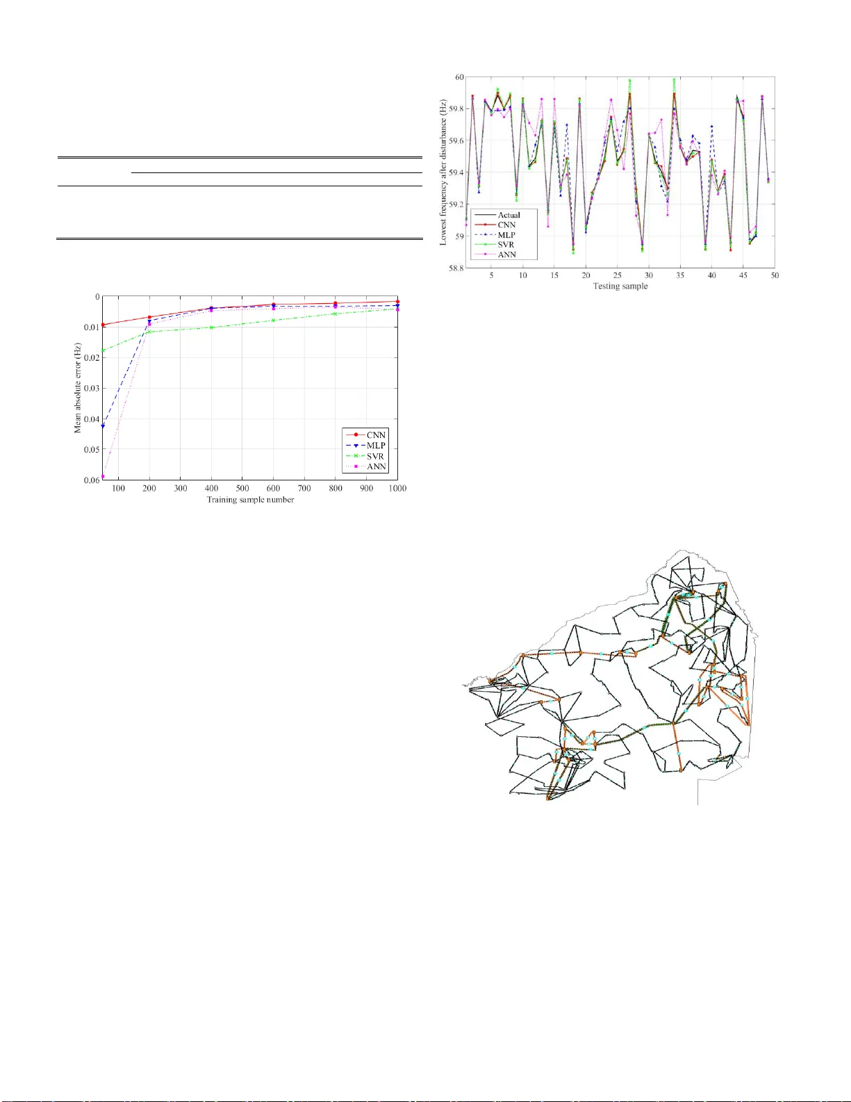
Abstract — The significant imbalance between p ower generation and load cau sed by severe disturbance may make the p ower system unable to maintain a steady frequency. If the post-disturbance dynamic frequency features can be predicted and emergency c ontrols are appropriately taken, the risk of frequency instability will be greatly reduced. In this paper, a predictive algorithm for post-disturbance dynamic frequency features is proposed ba sed on convolutional neural network (CNN) . The operation data before and immediately after disturbance is used to construct the input tensor data of CNN, with the dynamic fre quency features of the power system after the disturbance as the output. The operation data of the power system such a s generato rs unbalan ced power ha s spatial distrib ution characteristics. The electrical distance is pr esented to describe the spatial correlation of power system nodes, and the t -SNE dimensionality reduction algorithm is used to map the high-dimensional distance information o f nod es to the 2 -D plane, thereby constructing th e CN N input tens or to reflect spatial distribution of nodes operation data on 2-D plane. The CNN with deep network structure and local connectivity characteristics is adopted and the network parameters are train ed b y utilizing the backpropagation-gradient d escent algorithm. The case study results on an improved IEE E 39-node s ystem and an actual p ower grid in USA shows that the proposed method can predict the lowest fre quency of power system after the disturbance accurate ly and quickly. Index Terms — Convolutional neural network, deep learni ng, features prediction , dynamic frequency, power system. I. I NTRODUCTIO N ith the construction of the ultra -high -voltage AC and DC tran smission lines an d the integration of lar ge -scale Manuscript received June 3, 2019. This work was supported i n part by the laboratory foundati on project of China Electric Power Research I nstitute u nder the project of Fr equency Stability Ev aluation a nd Control of N ew Energy Integrated Power Sy stem Ba sed on Machine Learning under Grant FX83- 18 -00 2. Jintian Lin is with Electric Power Research Institute, State Grid Zhejiang Electric Power C o.,Ltd. , Hangz hou, CO 310000 Chi na ( e-mail: jtlin@my.swjt u.edu.cn ). Yichao Zhan g is with Sch ool of Elect rical Engineeri ng, Southwest Jiaotong University, Chen gdu, CO 610000 China ( e-mail: yc zhang_swjtu@163.c om). Xiaoru Wang is with School of Electrical Engineeri ng, Southwest Jiaotong University, C hengdu, CO 610000 China(e-mail: xrwang@hom e.swjtu.edu.cn). Qingyue C hen is w ith S chool of Electrical Engineering, Southw est Jiaoton g University, Chengdu, CO 610000 China(e-mai l: chenqi ngyue1995@163.c om). renewable energy in to th e power grid, the frequen cy dynamic behavior of the power system is bec oming more comp licated, which brin gs new ch allenges for p ower system s frequency stability. On the one hand, th e tripping of hig h -capacity generator s and large-scale renewable en ergy units, the damage of transmission corridor and the system splitting may cause serious imbalan ce of active power [1-2] . On the other hand, The decrease of system ine rtia, the incompatibility of operatio n and control strategies, and the increase of random fluctu ation intensity caused by renewable energy have also brought serio us challenges to power system freq uency analy sis and control [3] , which makes frequency stability problem becoming increasingly prominen t. System dynamic frequency refers to the p rocess of frequency variation with time caused by unbalanced power [4] . After the power d isturbance of system such as machin e tripping, the frequen cy of the system will first drop to a minim um frequency, and t hen the freq uency is restored to a quasi -steady state v alue b y th e primary frequency control. The dynamic fr equency features of the power system mainly includ e the lowest frequency and the steady - state frequency after the disturbance. A low frequency nadir can l ead to the disconnection o f generators, load shedding interv ention, and is therefore dangerous for system stab ility. Therefo re, fast and accura te prediction o f p ower system d ynamic frequency features in a ver y short tim e after the d isturbance occurred an d the s ystem is far from unstable is of great sign ificance f or implementing correspond ing em ergency frequency control strategy such as autom atic load sheddin g and emergen cy DC power support, ensuring s ystem frequency stability and preventing system frequency from collap se. At present, the p ower system dynamic fr equency analysis is generally based on time domain simulation [5] . Constrained by the calculation speed and the modeling accuracy, it can not meet the requirements of large power grids online prediction. In addition, some method s for fast dynamic frequency p rediction, such as equivalent model method, linearization method are proposed [6-8] ， wh ich simplify the system mod el an d obtains very fast calcu lation sp eed. Howev er, d ue to a larg e amount of equivalent, these methods have relatively large prediction error inevitably. With th e increase of power grid co mplexity and the decrease of system inertia ca used by ren ewable energy integration, higher requirement for o n -line fr equency prediction is put forward. The curren t methods based on po wer system physical model are d ifficult to balance bo th ac curacy Post-Disturbance Dynamic Frequency Features Prediction Based on Convolutional Neural Network Jintian Lin, Yich ao Zhang, Xiaoru Wan g*, Senior Me mber, IEEE , and Qingyue Chen W and computatio nal efficiency. The continuous improvement of the intelligent level of the power sy stem and the deep integratio n of the power system with th e Intern et and the communication network prov ides an information foundation for the data -driv en online power system frequency prediction m ethod [9] . Taking the system op erating state closely related to the disturban ce degree as input, the data-driv en model is used to construct the relationship from the input to the output frequency features, so that the influen ce of the disturbance is taken into acco unt in the model and the fast prediction is realized. Some data-b ased sh allow m achine learning methods such as sup port vector machines [10] , artificial neural netwo rks [11] and decision tree [1 2] has been app lied in power system fr equency prediction . However, due to the limited feature extraction ability of shallow machine learning methods, its ability to solve complex regression an d classification problems is constrain ed, and they ca nnot effectively mins and utilize and s patial -temporal correlation features ex isting in the power system operation data. In recent years, deep learning [1 3] has subverted the dominance o f shallow learning meth ods in many fields due to its excellent featur e e xtraction, classification and prediction ability. I t is w idely used in man y fro ntier fields such as computer vision [14] , natural language pro cessing [15] and speech recognition [16] . It also provides a new way of thinkin g for power system frequ ency analysis. Con volutional neural n etwork (CNN) is a r epresentative d eep learn ing framework, which can build a d eeper mach ine learning network with multiple hidden layer, and th e train ing algor ithms that adapt to the deep network is used to train the massive data sam ples to ex tract the spatial features of the power sy stem operatio n data, thereby f urther improving the accuracy of power system fr equency pred iction . Besides, CN N extracts the feature of data b y local receptive field, wh ich is especially suitable to pro cess data with spatial correlation features. Combined with the characteristics of power system operation data, the idea of ap plying CNN for frequency prediction emerges. In this paper, a po st-disturban ce f requency fea tures prediction method based on co nvolutional neural network is proposed. Th e method uses the elec trical distance b etween nodes to d escribe the spatial distribution of power system buses . The dimen sionality reductio n algorithm based on t-distributed stochastic neighbor embedding is used to map the high-d imensional spatial distribution of no des to the two-dimen sional coordinates. Based on the 2-D coo rdinates of the power sy stem nodes, the appropriate power system operating features are selected to construct th e tensor input of co nvolutional n eural networks. The CNN f rame is used to extract the hidd en abstract feature from the tensor input, thus the p ower system post-d isturbance frequency features prediction mo del is constructed . The case study r esults of an improved New Englan d 39 -nod e system with win d farm integrated and an actual p ower grid of USA show that the CNN method significantly im proves the predictio n accuracy compared with the traditional shallo w- structure frequency prediction method (SVR, AN N). Besides, comp aring the d e pth learning method ( MLP ) with fully connected network an d vector as input, the locally connected CNN with tensor data as input also has higher prediction accu racy benefits from its ability o f ex tracting spatial cor relation features . I n addition, CNN maintains g ood ac curacy under small training samples and unbalan ced samples. II. C ONVOLUTIONAL N EURAL N ETWORK Convolution al n eural network is d eep neural network with multiple layer and convolutional structure. The response of each layer of the CNN is excited by the local receptive field of the up per layer . CNN extracts the features of the input through the altern ately conn ected convolu tional layer and sub sampling layer, and passes abstrac t features to th e fully connected neural network for regression an d classification analy sis. A typical LeNet-5 [17] convo lutional neural network diagram is sh own in Fig. 1, w h ich incl udes in put la y er, s everal alternately connected convolutional and subsamp ling layers, fully connected layer, and output lay er. C3: f. maps 16@10*10 S4: f. maps 16@5*5 INPUT 32*32 C5: layer 120 OUTPUT 10 Convolutions Convolutions Subsampling Subsampling Fully Connected S2: f. maps 6@14*14 C1: feature maps 6@28*28 … Fig .1 Structure of LeNet-5 convoluti onal neural networ k . A. Structure of CNN 1) Input lay er: The input to th e CNN is ten sor d ata. Fo r example, the color images are th ird-order tensor data obtained by s uperimposing the seco nd-order tensor f eature maps of three RBG ch annels, and the element s in the tensor matrix are the color values of the pixels. The con cept o f tensor is exten ded to the f ield of power system. The ac tual p ower system can be approximately regarded as distributing on a 2 -D plane, an d the nodes of th e power system are similar to the imag e p ixels. Using power system operation features to construct several two-ord er tensors, b y superimpo sing these tensors, the third-o rder tensor input of th e CNN can be obtained. feature tensor 1 10× 10× 3 3 rd -order power system tensor data Nodes status value Channel R Channel G Channel B feature tensor 2 feature tensor 3 Fig.2 Analogy from RGB c olor images to t hird-order tensors of power systems. 2) Convolutional layer: The conv olutional layer is sparsely connected to the local area of the pr evio us feature map by the convolution k ernel, as shown in Fig. 3. Th e convolution kernel is a weigh t matrix which s lides with a certain strides on t he feature map, and performs discrete co nvolution calculatio n on the date in the local ar ea of the conv oluti on kern el. The calculation result is transmitted to a non -linear activation function and generates th e feature map of the next layer . For each feature map, the weight of the convolution kern el is constant, called the weight sharing principle, by which the amount of p arameters for training can be g reatly reduced. Strides=2 Strides = 2 Previous feature map Next feature map F ig . 3 Schem atic diagram of local receptive fie ld and convolutio n kernel. The calculation of the convolution layer is shown in equation (1): 1 i l l l l j i j j iM X X K b  −   =  +     (1) Where l j X is the ou tput of convolution al layer ; l is the layer number; j represents the j -th con volution k ernel, each convolution kernel corresponds to an output tensor feature map; 1 l i X − is the i -th feature map of previous lay er. i M is the se t of input feature map s. l j K is the weight matrix of convolution kernel;  is the two -dimension al discrete convolution operator; l j b is the bias value;  is the nonlin ear ac tivation function, usually ad opts ReLU fu nction. 3) S ub sampling layer: The s ubsampling layer is usually after the co nvolutional layer. The outp uts of the subsampling layer are also sparsely co nnected to upper lay er feature map, and the locally connected area do not overlap . The subsampling layer performs pooling operation on th e loca lly co nnected are a, the pooling metho ds includes maximum pooling , av erage pooling, random pooling , as is shown in Fig . 4. The subsam pling layer reduces the size of the feature map while maintain s th e feature scale to a certain ex tent, and can also avoids over -fitting problem and red uces comp utational exp ense. The calc ulation of the subsamplin g layer is shown in equation (2). ( ) ( ) 1 l l l l j j j j X do wn X b  − =+ (2) Where, l j  is the weight of subsampling area; l j b is th e bias of subsampling layer; ( ) dow n is the subsamplin g function. Max pooling Strides=3 Fig. 4 Schemat ic diagram of th e subsampling la yer and poolin g operation 4 ） Fully co nnected lay er: After several alternately connected convolution - subsam pling layer, the resulting feature m ap is input into the fully conn ected l ay er. In the fully conn ected layer, all abstrac t featur es in tensor map s are stretch ed an d converted into vector as inputs to a fully connected neural network to obtain the final classification or regression results. The calculation of the fully connected lay er is as follows: ( ) 1 l l l l X W X b  − =+ (3) Where, l W is the weight of fully the connected layer; l b is the bias of the fully connected layer. B. Training o f CNN The CNN is trained by b ack propagatio n and gradient descent algorithm. Using the loss function to calculate the error between th e forward netwo rk output and the expected value . Taking th e mean square error as example, there is the loss function: ( ) 2 , , , 1 ( , , , ; , ) 2 K W b E K W b x y h x y   =− (4) Where, ( , , , ; , ) E K W b x y  is the prediction error corresponding to train ing sample ( ) , xy ; ( ) , , , K W b hx  is the network f eedforward ca lculation output co rresponding to input x ; y i s the exp ected output v alue. The back propagation algorithm is used to transm it the error back to the parameter s layer by layer, thus ob taining the partial derivative of each parameter to total error. The gradient descent algorithm is used to u pdate th e parameter s accordin g to a certain lear ning r ate. By th e iterative computation of backward propagation -gradient descent to minimize the error of the feedforward n etwork and complete th e training of CNN. III. CNN B ASED P OST - DISTURBANCE F REQUENCY F EATU RES P REDICTI ON M ODEL The input of t he CNN is ten sor data. Ho wever, the input feature to traditional machine learning model for power system analysis is usually the data in vector form, which cannot re flect the spatial correlatio n o f power system bu ses status, n or is it suitable as the input to CNN. Therefore, the power s ystem operation data nee ds to be constructed in to ten sor form. Then the CNN is used to extr act the ab stract features o f input data and construct mapping from the o peration data input in tensor form to the dynam ic frequency feature s af ter disturbance. A. Spatial Distribution of Nodes Based on Electrical Distance The p ropagation of electro mechanical disturbances in the power system causes the state valu e of the system nodes to exhibit signif icant spatial distribution character istics. The relationship and interaction between p ower system node s are determined by the elec trical distance of nod es [18] . The smaller the electrical distance, the closer the relationship between the nodes status, an d th e m ore obvious the mutual influence. The electrical distance also dete rmines the distribution of t he unbalanced power in each g enerator under disturbance, which is closely related to th e dynam ic frequency of the power system [19] . The elec trical distance can be used to describe the position relations of the nodes, which is defin ed as the connection impedance between nodes. According to the superposition p rinciple [20] , the electrical distances between the nodes can be o btained by eq uation (5). ( ) ( ) ij ii ij ij jj D Z Z Z Z = − − − (5) Where , ij Z is the element o f the node impedance matrix ; ij D is the electrical distance between the nodes i and j ; Fo r a po wer system with n nodes, ij D is an n-order square symmetric matrix, the n-dimensional vector of each r ow of the matrix represents the electrical distance of one node to other nodes, which form s a node distribu tion in n-dim ensional space. B. Dimensionality Red uction of Nodes Spa tial Distribution Based on T -SNE The nodes spatial distribution ex ists in n -dimen sional space is incon venient for processing and visual d isplay, and it is al so difficult to constru ct the tensor input of the CNN through it . The actu al power system n odes can b e approximated as b eing distributed on a two -dimensional plan e. Therefore, the idea of dimensionality red uction is naturally introduced here. As shown in equation (6). The nodes in high- dimensional space ij D is mapped to the 2-D plane Y by dimensionality reduction, while retaining the or iginal electrical distance relationship between nodes as m uch as po ssible. 2 11 12 13 1 11 12 21 22 23 2 21 22 31 32 33 3 31 32 1 2 3 1 2 n n n ij n n n n nn n n x x x x y y x x x x y y D x x x x Y y y x x x x y y                 =  =                 (6) t-distributed stochastic neig hbor embedding (t -SNE) [21] is a probability- based nonlinear d imensionality reduction algorithm, which is improved by stochastic neighbor embedding (SNE). It is well-suited for embedding high -dimensional data for visualization in a low -dimensional space of two or three dimensions, a nd it’s also one o f the most effective dimension reduction algorithms at present. The basic princip le of the SNE is to convert the Euclidean distance betwe en the respective nodes co ordinates in the high-d imensional and the low-dim ensional space in to the co nditional probability, an d try to minimize the dev iation o f the two co nditional probab ility, so as to maintain th e distance relationship b etween no des before and after d imensionality reduction. Redefining the electrical distance matr ix ij D as a high-d imensional spatial d ata X . The co nditional p robability | ji p between each row vecto r in the high -dimensional spatial data X is defined as: ( ) ( ) 2 2 | 2 2 exp 2 exp 2 i j i ji i k i ki xx p xx    −− = −−  (7) Where , i x a nd j x is the nod e in the hig h -dimensional space X , which is represented by the n -dimension al vector of the i -th and the j -th r ow of the high-dimension al space X ; | ji P is the con ditional probability that the node j x appears near the node i x ; i  is the variance of the Gaussian fu nction ce ntered on th e node i x ; ij xx − is the Euclidean distance between the node i x and j x . Assuming that the high-dimensional spatial data X of the power system nodes is map ped to Y in the low dimension, th en there is also the conditional probability | ji q in the low-dimen sional space Y : ( ) ( ) 2 2 | 2 2 exp 2 exp 2 i j i ji i k i ki yy q yy    −− = −−  (8) Calculating the Kullback-Leibler divergence between the two probability distrib utions to mea sure the deviation b etween the two probability distributions and set it as t he objective function C . ( ) log ji ii ji i i j ji p C KL P Q p q ==    (9) Minimize the objective function by th e gradient descent algorithm, thereby obtaining the optimal nodes co ordinates in low-dimen sional space. However, t he Kullback-Leibler d ivergence objectiv e function of SNE is asymmetrical, the penalty co efficient correspo nding to different distances are different, which makes the SNE algorithm tend to retain the local stru cture in high-d imensional data and ignore the global features, while the asymmetric o bjective function is also difficult to optimized. Besides, the "congestion problem" caused by the d ifferent characteristics of h igh- dimensional and low- dimensional space makes the bo undaries between d ifferent clusters in dimensionality reduction result very blurred. The t-SNE algorithm utilizes the joint p robability distribution to replace the conditional probability d istribution, thereby eliminating the asymmetry of the objective f unction. At the sam e time, the t-SNE algorithm uses th e Gau ssian distribution to co nvert the Eu clidean distance in th e high-d imensional space X , and uses the t-distribu tion with a freedom degree of 1 to replace the Gaussian d istribution in the low-dimen sional space Y , thereby, the close nodes in the high-d imensional space will be mapped closer in l ow -dimensional space, and n odes far away will be mapped farther, thus solvin g the problem of nodes co ngestion. The jo int probability of h igh -dimensional space and low-dimen sional space data is as follows ： || 2 i j j i ij pp p n + = (10) ( ) ( ) 1 2 1 2 1+ 1 ij ij ki ki yy q yy − −  − = +−  (11) Where , n is the number of nodes. The new objectiv e function is derived as: ( ) lo g ij ij i i j ij p C KL P Q p q ==    (1 2) By minimizing the new objective fu nction, the optimal 2 - D nodes coordinates Y after t-SNE dimen sionality reduction can be obtained by gradient descent algo rithm . ( ) ( ) ( ) 1 2 41 ij ij i j i j j i C p q y y y y y   − = − − + −  (13) C. CNN input te nsor construction To constru ct the tensor input of CNN, th e matr ix elemen ts corresponding to the 2-D no de coordin ates are mar ked in the tensor matrix and the elements are filled with th e power system operation data of the nodes to obtain the feature map in tensor form. . Since the 2-D spatial d istribution Y is a set of c oordinates in the interval o f   01 ， , the index of matrix elements are in tegers, in order to mark the elements in the ten sor matrix corresponding to n odes coordinates, ch oosing an appropriate integer h and then the 2- D coo rdinates of nodes are enlar ged to the interval of   1, h by linear norm alization, Round the normalized nodes coordinates and the and the coo rdinates int Y of the integ er form are obtained. As is shown in equation (1 4 ). ( ) ( ) min int max min 1 1 h Y Y Y round YY −−  =+  −  (1 4) Construct a tensor matrix of size hh  , The operation status value of power system nodes is assigned to the tensor matrix elements correspon ding to the nodes coordinates int Y , and assigns remaining matrix elements that do n ot co rrespond to the nodes to 0, thus a tensor fea ture map correspon ding to a power system o peration featu re data is con structed, as is sho wn in equation (1 5 ). ( ) in t, 1 in t, 2 , , , 1 , 2 , , t t i i i M Y Y S t T i n =  = (1 5) Where int, 1 i Y and int, 2 i Y are th e abscissa and ordinate o f the i -th power system node; ( ) in t, 1 in t, 2 , t i i M Y Y is the value o f ten sor matrix elemen t corresponding to the node coordinates; t is the type of power system operation featu re; t i S is the op eration feature valu e of the i -th power sy stem node; T is the set of power system o perating data type . Inspired by the tensor data of the RBG colo r map, differen t power system features are assigned to several s econd -order tensor featu re maps, and these featu re maps are super imposed to construct th e third-ord er tensor input to the CNN .   INPUT 1 2 t M , M , , M = (1 6) D. Input fea ture selection In o rder to balance the accuracy an d th e training efficiency of the CNN, it is necessary to s elect the appropriate po wer system operation feature that affects the dynamic frequency of the power system as th e input to CNN. During the dynam ic pro cess o f the power system, the frequency of the system f luctuates ar ound the in ertia center of the sy stem [22] . The inertial center frequency is usually used to represent the global characteristics o f the power system dynamic freq uency, which is defined as follows: ( ) 1 1 n ii i sys n i i H H   = = =   (1 7) Where, sys  is the system inertia center f requency; i H is inertia time constant of the i -th g enerator in power system; i  is the frequency of the i -th g enerator in system , an d the generator s of the nodes are located at nod es . Defining the moment before the distur bance occurs as 0 t , and the m oment after th e disturb ance occurs as f t . I n the first stage of the p ower system dynamic process, that is, at the moment when the disturbance occur s, the generators will assume the unb alanced power according to the respective synchron ization coefficients, wh ich is r e lated to the initial operation state of the g enerators and the electrical distance to the fau lt poin t [18] . The synchronization co efficient sik P between the generator nod e and other nodes is def ined as: ( ) cos si n sik i k ik ik ik ik P V V B G  =− (1 8) Where, i V , k V and ik  are the voltage amplitude and p hase difference respectively; ik B and ik G are the transfer impedance. On this basis, th e electromagn etic power of each generator , the active power o f each loa d a t the m oment 0 t , an d the voltage and p hase angle of each n ode and the unbalan ced power of each generator at the moment f t are selected as inp ut f eature. In th e second stage of the po wer system dynamic process, the generator rotor is affected by the unbalanced power an d begins to gradually c hange the speed. The power s ystem dynamic frequency is directly determined b y th e motion equatio n o f the generator rotor, for the multi-m achine p ower system, there is the dynamic fr equency equation as fo llows [2 3] : 1 1 1 1 2 n n n s y s mi ei i i i i sys P P D H  = = =  = − −      (1 9) Where, sys H is the sum of the generato rs’ inertia time constants; mi P and ei P are the electromagnetic power and mechanical power of gener ators, D is g enerator damping coefficient. According to the dynamic frequency equation (1 9) , th e electromagn etic power an d mechanical power of the g enerators at the moment f t are selected as input feature. In order to reflect the in fluence of th e generators with d ifferent inertia to the dyn amic frequency, the response of each gen erator to the frequency ar e introduced [1 1] . 11 22 nn mi e i mi ei i i i i sys PP PP f HH == − − =−  ( 20 ) In the third stage of the disturb ance, the prime mover s and governor begins to r espon se to the frequency fluctuation, and the frequency is gradually restored by regulating the prime mover's o utput. The effec t of the regulatio n is affected by the reserve capacity and th e dynamic charac teristics of the prime mover s and governors . Traditional frequency response models based on equ ivalent physical mod el ignore the nonlin ear links such as th e limiter of the gover nor, and th e influence of the reserve capacity of the g enerators cannot be tak en into acc ount. Therefore, the spare capacity of the generators ri P at the moment f t is introdu ced here as th e input featu re , which is defined as: max ri i ei P P P =− ( 21 ) Where ri P is the reserve capacity of each generator ； max i P is the rated active p ower output of each gener ator. Besides, considerin g the frequency and voltage - dependent characteristics of the load, the load po wer of each node are selected as input f eature. Based on the analysis ab ove, t he original input feature set for dynamic frequency prediction is obtained, which consists of 1 4 power system o peration features. As shown in the table b elow. TABLE I O RIGINAL I NPUT F EATURE S ET FOR D YNAMIC F REQUENCY P REDICTION Number Input Feature type 1 Electromagnetic power of each generator at 0 t 2 Mechanical power o f each genera tor at 0 t 3 Reserve capacit y of each genera tor at 0 t 4 Voltage amplit ude of each node at 0 t 5 Voltage phase a ngle of each no de at 0 t 6 Load active power at 0 t 7 Electromagnetic power of each generator at f t 8 Mechanical power o f each genera tor at f t 9 Reserve capacit y of each genera tor at f t 10 Power shorta ge of each generat or at f t 11 Response of gen erators to distur bances at f t 12 Voltage amplit ude of each node at f t 13 Voltage phase a ngle of each no de at f t 14 Load active power at f t In o rder to reduce the occupancy of compu ter storage space and improve the training efficiency of CNN, b ased on the collected operation data of power system. The spearman correlation [2 6] coefficient is used to evaluate the correlation between each type of input feature and the dynamic frequency features after disturban ce and th e input features is further selected according to the correlation analysis result. The spearman co rrelation coefficient is defined as : ( ) 2 2 6 1 1 i s d NN  =− −  ( 22 ) Where, s  is the spearman correlation; i d is the difference between the rank order of input feature and frequ ency freture ; N is the numb er of samples. E. Frequency prediction modeling The construction process of the po wer system disturbance frequency prediction model based o n CNN is shown in Fig .5 and the spec ific steps are as follows ： 1) Obtaining the power system node s adm ittance matr ix according to th e t o pological relationship of the nodes and branches, inverts it and g et the node s imp edance matr ix. Using the n ode impedance matrix to calculate th e electr ical distan ce between nod es by equation (5) to describe the nodes distribution in high-dimen sional space. 2) The t-SNE algorithm is used to reduce th e dimensionality of nodes spatial distribution and map it to 2 - D plane. The nodes coordinates obtain ed after dimensio nality reduction are normalized and rounded to get the integer coor d inates between the interval [1, h ] accord ing to equation (1 4). 3) Gathering the power system operation data during the disturbance through the measurement equip ment or the offline simulation. Select the operation data of nodes in Table I to form the original inpu t feature data in v ector form, selected dynamic frequency features as output data. Perform data pre -pro cessing such as data clean ing and normalization. 4) Constructin g a matrix of si ze hh  , assigns the selected operation features to the matrix elem ents corresponding to the coordinates of the nodes, and obtain s the input samples of the CNN in form o f third-ord er tensor. 5) Th e ten sor input samples are d ivided into tr aining set and testing set in propo rtion by random samp ling , using the training set to train the p arameters of the CNN. 6) Using th e train ed CNN model to p redict the post-disturb ance dynamic f requency feature s of the test set and evaluate the prediction accuracy. Power system topology High-dimensional distribution of nodes based on electrical distance Two-dimensional nodes coordinates T-SNE Dimensionality Reduction Actual measurement/ offline simulation Power system Original operation feature gathering and selection Data Processing and normalization CNN Input tensor sample construction Power system disturbance Training sample set Testing sample set CNN frequency prediction model training Trained frequency prediction model Prediction results Fig .5 Constructio n process of the power system post-disturbance freq uency prediction model based on CNN. IV. C ASE S TUDY In ord er to test the performance of the proposed power system dynam ic frequency features prediction meth od based on CNN, an im proved New England 39 -node system with wind farm integrated and an p ower gr id of an actu al state in the United States is used for case study. A. Improved New En gland 39 -node system with wind farm integrated 1) S ystem introductio n The improved New England 39-node system with wind fa rm integrated has 11 generators and 40 nod es. Am ong th em, the No. 30 -39 nodes ar e conventional g enerators, and the No. 40 node is a wind farm with a rate d capacity of 90 0 MW. Th e t otal active po wer output of the generators in the initial operation mode is 6206 MW. The wiring diag ram of the system is shown is Fig. 6. G G G G G G G G G G 30 2 1 3 39 4 14 15 9 8 7 31 32 34 33 35 22 13 24 16 21 38 36 23 5 6 25 37 26 27 28 29 17 11 10 20 19 18 40 Fig .6 Wiring diagr am of the impr oved New Eng land 39-node test system. 2) I nput tenso r data construction The system is set to operate at 20 load levels from 50% to 100% . Un der different load levels, set the generators tripping faults and load fluctu ation disturban ces occur at 0 second, the system operati on features in Table I are r ecorded as CNN inp ut. The lowest frequency feature of the system after the disturbance are r ecorded as output. The simulation duration is set to 60 seconds. A total of 1400 sets of data are generated by simulation softwar e PSS/E. Using the spearman correlatio n coefficient to evalu ate the correlation between each type of feature and the lowest frequency after disturban ce. Accordin g to the spearman correlation analysis results, s ix input operatio n features with th e highest frequen cy correlation coefficient are fu rther selected as the inp ut feature to CNN, as is shown in Table II. Each type o f input feature is linearly normalized to the [0,1] interval to eliminate the ef fect of the feature d imension. TABLE II I NPUT F EATURE F URTHER S ELECTED BY S PEARMAN C ORRELATION Input feature t ype Spearman correl ation coefficient response of generators to distur bances at f t 0.5591 power shortage of each gener ator at f t 0.4731 voltage phase a ngle of each no de at f t 0.4107 electromagnetic power of each generator at f t 0.3613 electromagnetic power of each generator at 0 t 0.2913 load active power at f t 0.2898 Calculating the electrical distance between nodes to form the high-d imensional nodes spatial distribu tion X , as shown in Table III : TABLE III H IGH -D IMENSIONAL N ODES S PATIAL D ISTRIBUTION Node number Electrical dista nce between nodes (  ) 1 2 3 … 38 39 40 1 0 0.0322 0.0387 … 0.1017 0.0216 0.1312 2 0.0322 0 0.0122 … 0.0724 0.0420 0.1070 3 0.0387 0.0122 0 … 0.0737 0.0448 0.0997 … … … … … … … … 38 0.1017 0.0724 0.0737 … 0 0.1094 0.1572 39 0.0216 0.0420 0.0448 … 0.1094 0 0.1359 40 0.1312 0.1070 0.0997 … 0.1572 0.1359 0 The t-SNE dim ensionality reduction algorithm is used to map the high-d imensional n odes sp atial distribution to the 2 - D space Y , and the 2-D coordinates in Y are linearly nor malized to the interv al [1,100] an d rounded. As sho wn in Tab le IV . TABLE IV T HE E NLARGED 2-D N ODES C OORDINATES AFTER L INEAR N ORMALIZATION Node number T he enlarg ed two-dimensio nal coordinates of nodes int , 1 i Y int, 2 i Y 1 54 84 2 65 41 3 67 14 … … … 38 1 47 39 51 100 40 6 78 The distribu tion figure o f n odes in the 2- D plane is draw according to th e coordinates in Table IV , as shown in Fig. 7. Fig. 7 Distribu tion figure of nodes The effect of t-SNE dimensionality reduction can be visually reflected in Fig. 7 . Taking n ode 15 as an ex ample, the electri cal distances o f th e node 15 to nodes 14, 17, and 18 are 0.0163, 0.0145, and 0.0188 , respectively. C orrespon dingly, the node 15 is mapped clo ser to these nodes after d imensionality reduction . The electrical distances from node 15 to nodes 36, 3 7, and 38 are 0 .0553, 0.0554 , and 0.081 3, respectiv ely, and the y are mapped furth er in the two- dimensional plan e. Define a matrix M of size 1 00 10 0  , an d mark the elements ( ) int, 1 in t, 2 , ii M Y Y in the matrix corresponding to the 2-D coordinates of the nodes. Assigning one kind of input feature of the nodes to the corr esponding matrix elements, thereby obtain ing a second -order tensor feature map corresponding to the feature type. The seco nd-order tensor feature map s corr esponding to six input feature of po wer systems are superimpo sed to obtain a third-o rder tensor data of size 1 00 1 00 6  . Fig. 8 visually shows a second-ord er ten sor data co rresponding to the phase angle of each node at f t (generator tripping at No.30 node, load level 100 %). T he elements are given different colors according to th e input operation feature valu es. Fig. 8 Visualization of the tensor data corres ponding to nodes voltage phase angle. Reconstruct all 1400 sets of simulation data in to third -order tensor data and the input sample d ata of the CNN is o btained. 3) P ost-disturban ce frequency feature predictio n Randomly selecting 1000 samples as tr aining samples, and the remaining 400 are used as test samples. Th e CNN, multi-layer perception (MLP), support v ector regression （ SVR ） , and a rtificial neural networ ks (ANN) are used to predict th e lowest freq uency after power system distur bance respectively. Among them, MLP is a fully co nnected neural network with deep structur e, ANN and SVR are shallow machine lear ning model. At present, the h yperparameters of the d eep learning model can only b e determin ed by repeated test, that is, chan ging the hyperparameter s of the network for tr aining, and selecting the set o f hyperparameters with the relatively smallest erro r and t he best prediction result. According to a series of tests, t he hidd en layer of the convo lutional n eural n etwork is set to 5 layers, which are convolution layer, sub sampling layer -convolution layer, subsamplin g lay er and fully co nnected layer. Th e number of con volution ker nels or pooling kernels of each layer is 32 - 32 - 64 -64 respectively , the numb er of neuro ns in the f ully connected lay er is 256. The windo w size of the co nvolution kernel is 10 × 10 , the sliding st rides of wind ow is 1, t he convolution kernel activatio n fu nction is ReLU, the subsampling window size is 2 × 2, the win dow sliding strides is 2, and the subsampling m ethod adopts the maximum poo ling. The activation function of the fully connected layer is the Tan h function. The back ward propagation -gradient descent algorithm is used to [2 4] is used to update the network parameters. The learning rate is 1e -6 and the training epoch is 1 000. Referring to the structu re of the CNN, the hidden layer of the MLP is set to 5 layers, and the number of neurons in each layer is set to 32 - 32 - 64 - 64 -256 accordin g to the k ernels and neurons in each layer of CNN. Both MLP an d ANN are trained by gradient descent algorith m. The suppo rt vector regression model uses the velocity modified particle Swarm op timization (MVPSO) [25] to search fo r the optimal penalty facto r and radial basis kernel fu nction parameters. Using each trained machine learning model to predict the testing sample, Based o n pred iction results o btained by different model, the m ean a b solute er ror (MAE), mean absolute percentage error (MAPE) and root m ean squ are erro r (RMSE) are used to evaluate the prediction accur acy. The above accuracy indicato rs are d efined as follows: ( ) 1 1 MA E = N ii i f x a N = −  ( 23 ) ( ) ( ) 1 1 MAPE = N ii i i f x a N fx = −  ( 24 ) ( ) ( ) 2 1 1 RMS E N ii i f x a N = =−  ( 25 ) Where N denotes the number of test samples, ( ) i fx denotes the lowest freq uency pr edicted, i a denotes ac tual lowest frequency after disturban ce. Considering the randomness o f the train ing process, r epeat the tr aining p rocess for several times, and the average error analysis results ob tained are shown in th e Table V: TABLE V A CCURACY A NALYSIS R ESULTS O F D IFFERENT P REDICTION M ETHOD Prediction method MAE/Hz MAPE RMSE CNN 0.0018 3.0698e- 05 0.0024 MLP 0.0030 5.0298e- 05 0.0109 SVR 0.00 41 6.8178e- 05 0.0105 ANN 0.00 43 7.1977e- 05 0.0125 According to the accuracy analysis results, the proposed power sy stem post -disturban ce dynam ic frequen cy featu reslo prediction method b ased on CNN significantly improves the accuracy compared with the traditional shallow machine learning method (SVR, ANN). The mean absolute error of CNN compar ed to two above metho ds is reduced by 56.1%, 58.1, respectively . Compared with MLP with dee p network structure, the proposed method also has super ior per formance. On the one hand, the inp ut of MLP i s vector fo rm, which erases the spatial correlation information ex isting in d ata. On the other hand, the network of MLP It is fu lly conn ected, an d it is mo re likely to have problems such as overfitting, wh ich affects the accuracy of the network. The tensor input with spatial features and the deep network structure with local co nnection s of CNN greatly improvs these problems. Since the large frequen cy disturban ces rar ely o ccurs in actual power system, the samp le for training is usually limited . Th e influence o f th e tr aining sample number on th e ac curacy of different prediction method is analyzed in this paper. The methods were train ed by 50, 200, 4 00, 600, 800, 1000 sets of samples, and th e same test set was used for p rediction. U sing the mean ab solute error to analyze the ac curacy of the prediction results. The mean absolute error under different number of tr aining samples is shown in Tab le V I. TABLE VI T HE A VERAGE A BSOLUTE E RROR OF T HE T EST S AMPLE C ORRESPONDING TO THE N UMBER T RAINING S AMPLES AN D D IFFERENT M ETHODS Prediction method Training sample number 50 2 00 4 00 6 00 8 00 1 000 CNN 0.0093 0.0068 0.0038 0.0027 0.0023 0.0017 MLP 0.0425 0.0080 0.0039 0.0032 0.0032 0.0030 SVR 0.01 77 0.0 116 0.0102 0.0079 0.0 057 0.00 41 ANN 0.0 588 0.0091 0.00 47 0.00 40 0.00 35 0.00 43 According to the accuracy evaluation results in Table VI, the prediction error of variou s machine learning methods und er different tr aining samples is shown in Fig. 9 Fig . 9 . Me an absolute error of di fferent methods with varying training sample number. According to the prediction accurac y analysis results shown in Tab le VI and Fig. 9, it can be seen th at with the incr ease of the number of training samples, the prediction accuracy of various machine learning models is grad ually increasing, under different sizes of training sam ples. The frequency pr ediction method based on CNN proposed in this paper has smaller prediction error th an oth er mac hine learning metho ds. In particular, in the case of only 50 training samples, the C NN method also has h igh accuracy, which has signif icant advantages over other m achine lear ning m ethods. The mean absolute error is reduced by 78.1%, 4 7.5%, and 84.2% compared to MLP , SVR, and ANN. Besides, MLP and ANN with fully connected network s hav e sever e ov er-fitting problem in the case of small sample size. Selecting 50 sample in the test set, as shown in Fig. 10 . It can be seen that the p rediction results of CNN are closer to the actual values than o ther metho ds. In addition, CNN method has a fast calculation speed , which only co sts 4 .063 ms for single prediction . The above an alysis shows the frequ ency prediction method based on CNN can analy ze the f requency af ter power system disturban ce qu ickly and accurately. Fig. 10 . Comparison of t he predicted resu lts with the actual values B. Actual po wer grid in the United S tates The actu al large power grid u sually has strong spatial distribution feature information. In order to test th e application ability of the CNN-based frequency predictio n method on the actual large power grid, this section introduces the actual p ower system of an ac tual state in the United States as an examp le. 1) System introduction The power system of this state has 500 n odes and the voltag e levels o f nod es ar e 345kV, 13 8kV, 1 3.8kV, there are 466 transmission lines , 131 transformers, and 90 generators in this power system, including thermal generators, h ydropower generator s and gas g enerators. Th e installed cap acity of the system is 14 626.74 MVA. The g eographic wiring d iagram of this actual po wer system is shown in Fig . 1 1. Fig. 11. Geograp hic wiring dia gram of an actual p ower system i n USA 2) Analysis of spatial distributio n characteristics of po wer system operation fea ture The operation feature of the actual large power grid disturbance appears a strong spatial distribution char acteristic. Firstly, the electrical distance is used to describe th e location relationship of each node in th e sy stem , an d then the t-SNE dimensionality reduction algorithm is used to map the no des to the 2-D space. The distribution of the power system nodes in the 2-D plane is as shown in Fig. 11. The spatial distributio n of the nodes can be clearly seen from the fi g ure , which can reflect the location r elationship of the nodes to a certain extent. Fig. 11 distrib ution of the pow er system nodes in t he 2 -D plane Using the same post-d isturbance operatio n data gener ation method to obtain 14 00 sets o f disturbance simulation data, and then th ese data is r econstructed into tensor form and the tensor feature m ap corr esponding to each typ e of operation d ata is obtained. Using the same post-d isturbance operatio n data gener ation method and input ten sor constr uction method, the sample data of CNN sam ples is obtain ed. Fig. 1 2 clearly shows th e operation status values o f n odes at differ ent lo cations o n a 2 - D plane under a certain disturb ance, wh ich f orming sev eral second-o rder tensor feature maps. They are the ge nerator electromagn etic power, the load active p ower and the node voltage phase an gle at the moment f t Fig.12 Power s ystem operation st atus feature ma p Fig. 13 shows the unb alanced power of each generator at the moment that the node 82 and n ode 439 occur s generator tripping fault. The matrix coordinates correspo nding to node No. 82 and the node No. 43 9 are (46, 65) and (9, 32), respectively. It can b e clear ly seen from the Fig. 13 that af ter the fault occurs, the nodes closer to th e fau lty no de is more affected by the fault, an d tend to assum e more unbalan ced power. This again proves that the CNN tensor input construction method propo sed in this p aper can maintain the spatial correlation inform ation o f the power system node operation data. Fig.13 Feature map of the unbal anced power under the fault at differ ent locations 3) Post-disturbance frequ ency prediction The power system o peration data in the form of th ird -ord er tensor is used as the input to the CNN, the lowest freq uency after the power system disturbance is used as the output. Randomly selecting 10 00 sets of samples as training samples, and the rest as testing samples. When training CNN, because this actual p ower system has a large number of nodes an d the nodes distribution is dense, the s ize of the convolution kernel is appropriately r educed to 5 × 5 to better mine s the local fea tures of the input , other hyperp arameter are the same as th e previous example. Using the trained CNN mo del to p redict the testing set, and the accurac y analysis result is shown in Table VI I. TABLE VI I A CCURACY A NALYSIS R ESULTS O F D IFFERENT P REDICTION M ETHOD Prediction method MAE/Hz MAPE RMSE/ Hz C NN 0.0021 3.4964e- 05 0.0030 M LP 0.0027 4.4204e- 05 0.0042 S VR 0.0032 5.3661e- 05 0.0037 A NN 0.0056 9.2802e- 05 0.0065 The accuracy analysis results of the testing sample show that the power system post -disturban ce frequency prediction method based on CNN also has high er accuracy when applied in the actual power system. Fig. 14 shows the predict ion results of the testing samples. As can be seen fr om the figure, the lowest frequency predicted by CNN mo del is very close to the ac tual simulation r esults. In addition, due to the large capacity of the system, most power fluctuations o nly cause sligh t frequency d isturbances, an d only a few power disturb ances cause large frequency deviation s, of which 7.75 % ex ceeds 0.1 Hz, an d 1.5 % exceeds 0.2 Hz. It can be seen th at in the face of such poorly balanced samples, the CNN m ethod also has a strong gen eralization ability, which c an accu rately p redict the lowest f requency f luctuation caused by large power distur bance. Fig. 14 Comparis on of CNN pre diction results and ac tual simulation values. V. C ONCLUSION CNN with its tenso r data input and deep network structure has ex cellent processing ability fo r sp atial co rrelated data . I n this paper, a CNN based predictive method for power system post-disturb ance frequency features is proposed . By constructing the power system o peration data into tensor form, the spatial correlation information o f th e o peration d ata is effectively retained in the CNN input data, thus laying a good foundation for the successful ap plication of CNN to the accurate prediction of post-disturbance frequency features. The case study shows the propose d f requency p rediction method significantly improves the accuracy compared to the traditional shallow mac hine learning meth od such as SVR, AN N. Compared to the deep learning MLP based method with fully connected network and vector as input, the proposed CN N based one also has higher accuracy due to its locally connected structure and tensor form input. Fur thermore, the proposed method has better perform ance of g eneralization ability in the case of small sam ples and unbalan ced samples of large power grid. Th e proposed m ethod can b e applied to the online frequency stability analysis of the actual power system . According to the prediction result s such as maximum frequency deviation, the corresponding emergency control such as automatic load shedd ing can be fo rmulated to prev ent the power system f rom frequency instability . R EFERENCES [1] Z. W. Li, X. L. Wu, K. Q. Zhuang, et al . “Analysis and R eflection on Frequency Characteristics of East C hina Grid After Bipolar Locking of “9·19” Jinping - Sunan DC Transmissi on Line,” Automation of Electric Power Systems , vol. 41, no. 7, pp. 149-155. Apr, 2 017. (in Chinese) [2] Z. J. Huang, X. Y. Li , J. Chao, P. Kang, “Guiyang south grid 7.7 faults simulation and a nalysis,” Automation of Electric Power S ystem , vol. 31, no. 9, pp. 95-100. May. 2007. (in Chi nese) [3] R. F. Yan, N, A, Masood, T, K , Saha, et al . “ The Anatomy of the 2016 South Australia Blackout: A Catastr ophic Event in a High Renewable Network,”. IEEE Transactio ns on Power Systems , vol. 33, no. 7, pp. 5374-5388. Sep, 2018. [4] Y. D. Han, Y. Min, X. N . He, et a l. “A new conce pt and algorithm for dynamic fr equency i n power systems ,” Automation of Elec tric Power Systems , vol. 17, no. 10, pp. 5-9. Oc t. 1993. (in Chines e) [5] C. Rehtanz. “Agent Technology Applied to the P rotection of Power Systems,” in Au tonomous systems a nd in telligent agents in power system control and oper a tion . Berlin, G ermany: Springer , 2003, pp. 115-154. [6] M. L. Chan, R. D. Dunlop, F. Schweppe. “Dynamic equivalents for average system freq uency behavior followi ng major disturbance,” IEEE Transactions on Power Apparatus and Systems , vol. PAS-91, no. 4, pp. 1637-1642. Jul, 1 972. [7] P. M. Anderson, M. M irheydar. “A l ow -order system frequency response model,” IEEE Transactions on Power Systems , vol. 5, no.3, pp. 720-729. Aug, 1 990. [8] M. L arsson, C. Rehtanz. “ Pr edictive fr equency s tability contro l based on wide-area phasor m easurements ,” in IEEE Power Engineering Society Summer Meeti ng , Chicago, I L, USA, 2002, pp. 2 33 -238. [9] Zhong Z, Xu C, Billian B J, et al. Power system frequency monitoring network (FNET) implementatio n[J]. IEEE Transa ctions on P ower Systems, 2005, 2 0(4):1914-1921. [10] Q. B. Bo. , X. R. Wang, and K. T. L. “Minimum frequency prediction based on v-SVR for post- disturbance po wer system.” Electric Power Automation Equipment , vol. 3 5, no. 3, pp. 83-88. Apr, 2 015. ( in C hinese) [11] M. B. Djukano vic, D. P. Popovic, D. J. Sobajic, et al . “Prediction of power system frequency resp onse a fter g enerator outages using neural nets,” IEE Proceedings C-Generati on, Transmissi on and Distrib ution , vol. 140, no.5, pp. 389-398. Sep, 1 993. [12] D. Lopez , L. Sigrist. “A centralized UFLS scheme using decision t rees for small isola ted power systems, ” IEEE Latin America Transactions , vol. 15, no. 10, p p. 1888-1893. Oct, 2017. [13] Y. Bengio. “Learning Deep Architectures for AI,” in Foundations and Trends i n Machi ne Learni ng , Oxfor d, U K: Oxford Univ Press, 2009, pp. 1-127. [14] W. S. Zhang, D. H, Zhao, G. W. Gong, et al . “Food image recognition with convolutional neural networks ,” in 2015 IEEE 12th Intl Co nf on Ubiquitous Intelligence and Computing and 2015 IEEE 12th In tl Conf on Autonomic and Trusted Compu ting and 2015 IEEE 1 5th Intl Conf on Scalable Computing and Co mmunicat ions and Its Associated Workshops (UIC -ATC-ScalCom) ， Beiji ng, China, 2015, pp. 690-693. [15] M. M ohamed. “Parsimonious memory un it f or recurrent neural n et works with application to n atural language processing, ” Neurocomp uting , vol.314, pp.48-64. Nov, 2018. [16] G. Hinton, L. Deng, D. Y u, et al . “Deep neural networks for acoustic modeling in sp eech recognition: the share d views of four rese arch groups,”. IEEE Signal Processing Magazine , vol. 29, no. 6. pp. 82 -97. Oct, 2012. [17] Y . Lecun, L . Bottou, Y . Bengio, et al . “ Gradient-based learning applied to document r ecognition,” . Pro ceedings of the I EEE , vol. 86 , no. 11 , pp. 2278-2324. Nov, 1 998. [18] Lagonotte, Sabonn adiere, Leost, et al . “Structural an alysis of the electrical system: application to secondary voltage control in france,” IEEE Transactions on Power Sy stems , vol. 4, no. 2, pp. 479 -486. May, 1989. [19] P. M. An derson, A. A. Foua d. Power Sys tem Control and Stability . New Jersey: IEEE Press , 2003, pp: 69-83. [20] E. Bompard, R. Napoli, F. Xue. “ Analysis of structura l vulnerability in power transmission grid,”. Internationa l Journal of Critical Infrastructure Pro tection , vol. 2, n o. 1, pp. 5-12. May, 2009. [21] L. V. D. Maaten, G. Hinton. “Visualizing data using t - SNE,” Journal of Machine Learni ng Research , vol. 9, no. 1, pp.1-48. Nov, 2 008. [22] Y. D. Han, Y. Min , X. N. He, et al . “A new concept and algorithm for dynamic frequency in power systems,” Automation of Electric Power Systems , vol. 17, no. 10, pp. 5-9. Oc t, 1993. (in Chinese) [23] P. Ku ndur. Po wer sys t em s t ability and contro l , New York, McGraw-Hill, 1990, pp. 128-136. [24] Diederik P K, Jimmy B. Adam: A Method for Stochastic Optimization. 3rd International Conference for Learning Representations. USA. San Diego, 2015. [25] Z. F. Qi , Q. H. Jiang , C. B. Zh ou, et al . “A new slope dis placement back analysis method base d on v -SVR and MVPSO algorithm and its application,” Chinese Jour nal of Rock Mechanics and Engineeri ng , vol. 32 , no. 6, p p: 1185-1196, 201 3. (in Chinese) [26] J. Hauke, T. Kossowski. “Compari son of values of pearson's and spearman's correlati on coefficients on the same sets of data,” Quaestiones Ge ographicae , vol. 30, no. 2, pp. 87-93. Jun 2 011. Jintian Lin received the B.E. degree and M.E. degree in Electrical Engineering from Southwest Jiaotong University, C hengdu, China in 2016 and 2019. And he is now working in Electric Power Re search Institute, State Grid Zhejiang El ectric Power C o.,Ltd. His research is mainly focus on the analysis of frequency stabilit y based on mach ine learning. Yichao Zhang received the B .E degree in E lectrical Engineering from the Southwest Jiaotong U n iversity, Chengdu, China, i n 2017. And she is currently pursuing M. E degree i n electrical engineering at Southwest Jiaotong Uni versity. She has been involve d in research on the anal ysis of fre quency stability based on t he machine learning. Xiaoru Wang received the B.E degre e and M.E degrees in El ectrical Engineering from Chongqing University, China, in1983 and 1988 respectively, and the Ph.D degree from Southwest Jiaotong University ,China, in 1998. She is cu rrently a Profess or a t the School of Electrical Engineerin g of Southwest Jiaotong Univers ity. Her research interests include power sy stem p rotecti on , stability analysis and control based on wide-area measurements. S he is senior memb er of IEEE. Qingyue Chen re ceived the B.E. d egree in Electric Engineering from Southw est Jiaotong University, Chengdu, China, in 2018. She i s currently pursuing the M.E. d egree in Electrical En gineering at Southwest Jiaotong University. Her current research interests include renewable energy generation and its frequency control.