On the Impact of Ground Sound

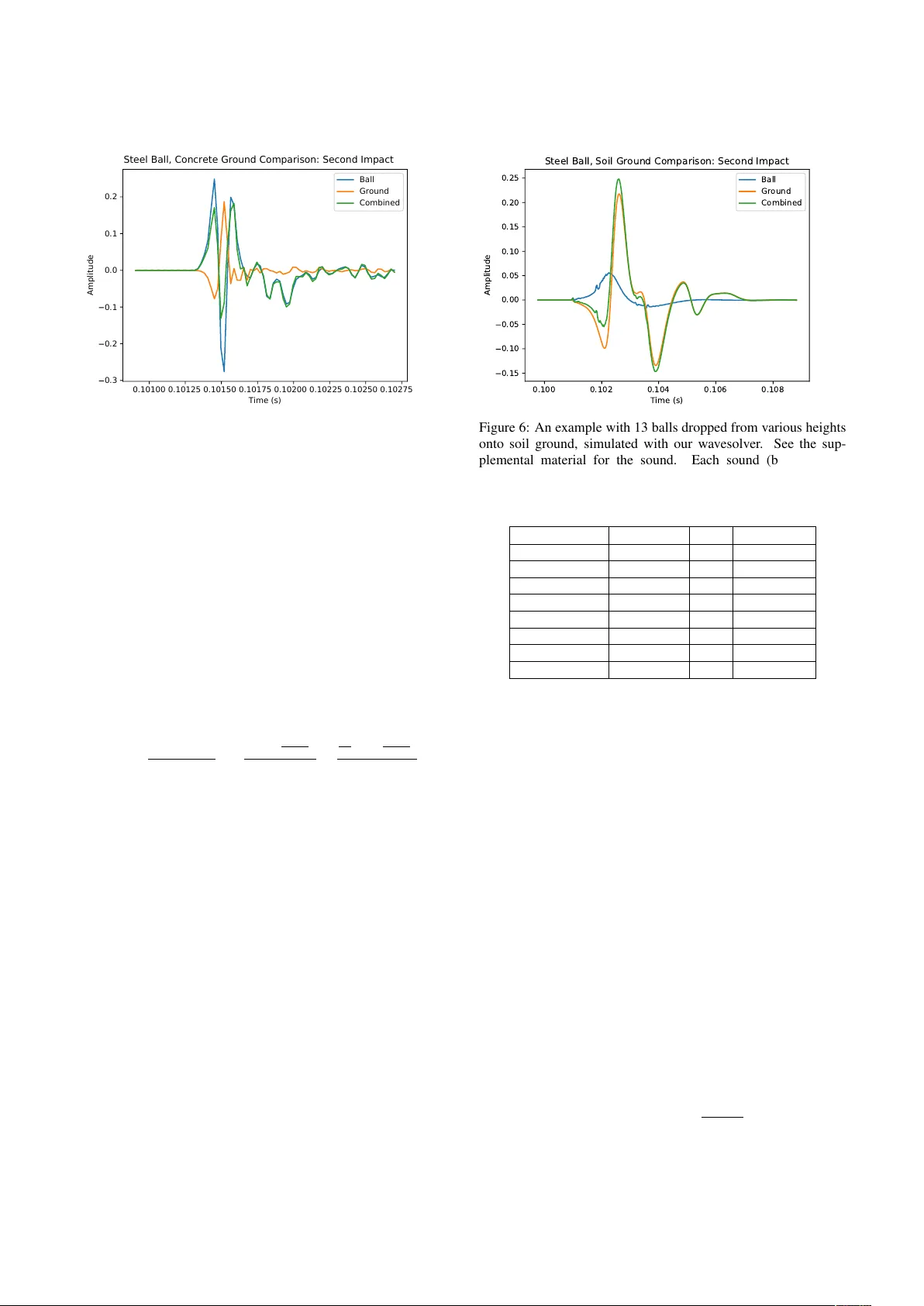
Pr oceedings of the 22 nd International Confer ence on Digital Audio Ef fects (DAFx-19), Birmingham, UK, September 2–6, 2019 ON THE IMP A CT OF GROUND SOUND Ante Qu and Doug L. J ames Computer Science, Stanford Univ ersity Stanford, CA 94305 [antequ|djames]@cs.stanford.edu ABSTRA CT Rigid-body impact sound synthesis methods often omit the ground sound. In this paper we analyze an idealized ground-sound model based on an elastodynamic halfspace, and use it to identify sce- narios wherein ground sound is perceptually relev ant versus when it is masked by the impacting object’ s modal sound or transient acceleration noise. Our analytical model gives a smooth, closed- form expression for ground surface acceleration, which we can then use in the Rayleigh integral or in an “acoustic shader” for a finite-difference time-domain wav e simulation. W e find that when modal sound is inaudible, ground sound is audible in scenarios where a dense object impacts a soft ground and scenarios where the impact point has a low ele v ation angle to the listening point. 1. INTR ODUCTION Many sound synthesis examples in computer animation and vir- tual environments contain moving objects that impact the ground or other large flat surfaces. The ground affects the sound in two ways: 1) as a passive scatterer: sound wav es in the room are re- flected off the ground, and 2) as an emitter: the surface of the ground vibrates due to impact e vents, and thus emits sound. T ypi- cal approaches incorporate the passiv e scattering and reflection de- pending on context and methodology; howe ver , very few physics- based approaches consider the acoustic emissions of the ground itself. In this paper we model the ground as an idealized elas- todynamic halfspace, and analyze its sound emission during an object-ground impact. Its relativ e importance is assessed in vari- ous object-ground impact scenarios, and is found to vary greatly . Ground emission and scattering hav e been explored in many works over the decades. One line of works [1, 2] fit data-driven models to synthesize footstep sounds. W orks on fracture and micro- collisions [3, 4] treat the ground and table as a large modal vi- bration source; of these, one paper [3] models the modes from a 9 m × 9 m × 0.9 m concrete slab; these dimensions directly af- fect modal resonant frequencies. The modal method also requires heavy precomputation resources and storage because lar ge objects hav e many vibration modes within audible frequencies. Further- more, the abov e methods [3, 4] compute propagation with only one object at a time and omit repeated object-ground reflections. After an object-ground collision, we may hear three types of sounds: (1) the object emits ringing sound from on its resonant modes, (2) the object emits a transient acceleration noise upon impact, and (3) the ground emits a transient sound upon impact. While many previous papers [3, 4, 5] model the first two in their Copyright: c  2019 Ante Qu and Doug L. James. This is an open-access article distributed under the terms of the Creative Commons Attribution 3.0 Unported Li- cense, which permits unr estricted use, distribution, and repr oduction in any medium, pr ovided the original author and source ar e cr edited. sound synthesis, they omit the third type of sound. Most recently , [5] models the collisions of many floor materials; howe ver , it in- corporates the floor properties only in the excitation force profile and models sound just from the object’ s surface. One argument for omitting the ground sound is that object sounds are often louder , especially for lar ger objects, and can mask quieter ground contributions. Nevertheless, depending on the floor- ing materials, contact parameters, and listening angle, the ground can sometimes be a more efficient sound source than a small ob- ject. The interference from the object’ s reflection can also change its wav eform and make it distinct from the ground sound. Our ground vibration model allows us to quantify the intensity of the ground sound, albeit for a simplified elastic halfspace ground model. Another work [6] develops a discretized modal model to col- lide vibrating strings with solid obstacles. W e aim not to model ringing sound but rather to introduce a closed-form formula for the transient surface vibrations due to a single impulse. Finite-difference, time-domain (FDTD), wa ve-based sound syn- thesis methods [7, 8, 9] naturally handle scattering with static or moving objects. Recently , [9] enabled scattering with moving ob- jects by rasterizing their boundaries during each timestep. This method abstracts away object sources using an “acoustic shader” interface; the simulation queries the object shader for the surface vibrations and uses them to driv e sound wa ves that propagate to the listener . Howe ver , no method is proposed to ev aluate ground vibrations in an acoustic shader . W e implement a ground shader in this work. Our work focuses on the topic of sound emission rather than reflections; it is orthogonal to room acoustics models that simulate room impulse responses and modes. This surface vibration problem has been studied in seismol- ogy literature as Lamb’ s problem [10], and its ideal solution is well-known with a closed form. Howe ver , the ideal solution to an instantaneous load contains singularities at wa vefronts that are difficult to ev aluate numerically . T o smooth the singularities, we deriv e a closed-form temporal regularization of the solution to Lamb’ s problem that remov es the singularities at the three wav e- fronts, similar to ho w [11] regularizes the singularity in an infinite elastic medium for animation effects. This closed-form expression makes it easy to model ground sound without simulation. W e consider the following problem: Given a simple solid ob- ject, such as a ball, colliding with the ground (modeled as an elastic half-space) how do we estimate the sound emitted by the surface vibrations of the ground? Our contributions are 1. an estimate of the material properties and object sizes where the ground sound is not masked by the object sound, 2. an interactive method to synthesize ground sound (no pre- computation is required), and 3. an “acoustic shader” for finite-dif ference time-domain sim- ulations that directly ev aluates the regularized solution. D AFX-1 Pr oceedings of the 22 nd International Confer ence on Digital Audio Ef fects (DAFx-19), Birmingham, UK, September 2–6, 2019 2. GR OUND SOUND MODEL: BA CKGR OUND W e model the transient ground sound by first modeling the ground surface vibration, and then using this motion to dri ve sound propa- gation into the air . For the former, we deriv e a closed-form model of the ground vibration to minimize computation while preserving accuracy . Our propagation model is one-way coupled because air pressure oscillations are not po werful enough to af fect the ground. In particular , we use Lamb’ s problem [10] and its solutions to model the floor surface vibrations from an impact, and we describe them in Sections 2.2 and 2.3. W e regularize the model in Section 3 to eliminate undesired singularities, and then we model the sound propagation in Section 4. 2.1. Lamb’ s problem W e present Lamb’ s problem here, which in volves applying an in- stantaneous normal point load to an elastic halfspace. W e present it with a load rather than an impulse in order to simplify the math- ematical representation of the solution. In later sections we will deriv e and use a closed-form representation of the surf ace acceler- ation in response to a specific impulse profile. Consider a linear isotropic elastic half-space with Poisson’ s ratio ν and stiffness (shear modulus) µ , as shown in Figure 1. W e consider the elastic half-space to be on the bottom ( z negativ e), and free space to be abov e it, with the boundary being the horizontal z = 0 plane. Starting at time t = 0 , a normal point force of magnitude 1 is applied and held (“push”) at the origin (0 , 0 , 0) . The input force profile on the z = 0 plane is therefore f ( x, y , t ) = δ ( x, y ) θ ( t ) ˆ z , (1) where δ, θ are the Dirac delta and Heaviside theta functions. f(t) + z u n (r,t) r ground air Figure 1: Notation for Lamb’s problem: f ( t ) is the ground ex- citation force, and u n ( r , t ) is the vertical displacement response. Note that while our diagram sho ws f ( t ) in its usual downward direction ( − z ), we define f ( t ) in (1) to point in the + z direction. The linear partial differential equations and boundary condi- tions can be found, for example, in equations 4 and 1 (respectively) of [12]; we present their closed-form solution in the next section. 2.2. Solution to Lamb’ s problem Pekeris [12] first solved Lamb’ s problem in 1955 for ν = 1 / 4 . Others [13] later solved it for generic ν . W e present the solution for generic ν from [14]. Some relev ant notation is the follo wing: c p = speed of compression (P)-wa ves in the medium , c s = speed of shear (S)-wa ves in the medium , a = c s c p = r 1 − 2 ν 2 − 2 ν , r = p x 2 + y 2 . Define κ 2 1 , κ 2 2 , κ 2 3 as the complex roots to the Rayleigh equation: 16(1 − a 2 ) κ 6 − 8(3 − 2 a 2 ) κ 4 + 8 κ 2 − 1 = 0 . (2) This equation admits three real solutions when ν < 0 . 2631 ; oth- erwise, it has one real root and two complex conjugates. Let κ 2 1 be the largest real root, and define γ = κ 1 . Treat these roots as math- ematical tools to help express the result with no direct physical meaning (except that γ is the ratio of the S- and R- wav e speeds). Define the following set of coef ficients: A j = ( κ 2 j − 1 2 ) 2 q a 2 − κ 2 j ( κ 2 j − κ 2 i )( κ 2 j − κ 2 k ) , i 6 = j 6 = k While the response contains both horizontal and vertical displace- ment, only the vertical motion produces sound. The final vertical displacement response u n ( r , t ) is the following: u n ( r , t ) = 1 − ν 2 π µr              0 τ ≤ a, 1 2  1 − P 3 j =1 A j q τ 2 − κ 2 j  , a < τ < 1 , 1 − A 1 √ τ 2 − γ 2 , 1 ≤ τ < γ , 1 τ ≥ γ , (3) τ = c s t r . (4) This solution applies for all ν , from 0 to 0 . 5 (see [14]). The piece- wise boundaries correspond to the three wav efronts: the pressure P-wa ve arri ves first, when τ = a , tra velling at speed c p . The shear S-wa ve arriv es when τ = 1 , travelling at speed c s . Finally , the Rayleigh R-wave arriv es when τ = γ , trav elling the slowest at speed c r = c s / γ . See the blue line in Figure 2 for an illustration. 0.6 0.8 1.2 1.4 t - 2 - 1 0 1 u ( t ) Surface Displacement due to Load, 1 m Away Original Pekeris ϵ = 0.02 m ϵ = 0.05 m ϵ = 0.10 m ϵ = 0.25 m 1.0 P R S Figure 2: Elastic wavefr onts in time: (Blue:) Scaled displace- ment response in the Pekeris solution, at 1 m away . The three wa vefronts (P-, S-, R-) are labeled. (Other colors:) Our temporal regularization, described in Section 3. The horizontal axis is time in seconds; the vertical axis is scaled normal displacement. Note: It is often conv enient to flip the signs of a 2 , γ 2 , and τ 2 in the square roots of both the numerator and denominator in the terms containing A 1 , so that the inside of the square root is real. 2.3. Singularities In order to radiate sound waves we need to ev aluate the acceler- ation in the impulse response of Lamb’ s problem. Unfortunately , the push-like load’ s displacement response, u n ( r , t ) , already con- tains four singularity locations, which means that at each singular- ity it will be difficult to numerically approximate surf ace motion. • One singularity occurs at all positive t at the origin, where r = 0 . This singularity occurs due to the spatial δ load location, and it has asymptotic behavior 1 / r . D AFX-2 Pr oceedings of the 22 nd International Confer ence on Digital Audio Ef fects (DAFx-19), Birmingham, UK, September 2–6, 2019 • One singularity occurs at each of the wav efronts—one each at the P- ( τ = a ), the S- ( τ = 1 ), and the R- ( τ = γ ) wa ve fronts. The first two wav efronts have continuous but not differentiable singularities. The third wav efront is dis- continuous with asymptotic behavior ( γ − τ ) − 1 / 2 . Our goal is to design a regularizing function in time or in space, as a smooth approximation of a delta impulse, to act as the initial force. W e then conv olve our function with the u n solution to get a closed-form response that remov es the singularities. W e consider the physical parameters of our problem in choos- ing temporal versus spatial regularization. W e would like the reg- ularization parameter to directly match the contact timescale and area. T ypical contact radii are much smaller than the contact timescale multiplied by any of the three wav e speeds; see T able 1 for one example. Therefore the spatial contact area smooths the resulting wa ve by v ery little compared to the temporal smoothing. T emporal regularization thus gi ves us a more accurate response than spatial. 3. TEMPORAL REGULARIZA TION OF THE GROUND VIBRA TION MODEL Consider a function f  ( t ) that approximates δ ( t ) on a smoothing timescale  . Since the elastic wav e equation is linear and u n is the response to a Heaviside θ load, we can get the vertical displace- ment response to the force, f  ∗ θ (which is an approximate θ ), by computing the con volution u  = f  ∗ u n , or u  ( r , t ) = Z ∞ −∞ f  ( t − t 0 ) u n ( r , t 0 ) dt 0 . (5) The above gives us the displacement response to a “push load” (c.f. [11]). W e want an impulse response corresponding to a f  ( t ) force profile. Since δ is the deriv ativ e of θ and f  can be written f  ∗ δ , we can subsequently compute the displacement response w  to an f  impulse force by taking a time deriv ati ve of u  , and like wise the acceleration a  by taking more deriv ati ves: w  ( r , t ) = ∂ u  ∂ t , (6) a  ( r , t ) = ∂ 3 u  ∂ t 3 . (7) W e use the regularization function f  defined by g  ( t ) = c s  π ( c 2 s t 2 +  2 ) ; (8) f  ( t ) = 2 g  ( t ) − g 2  ( t ) . (9) W e chose this function for sev eral reasons. Firstly , it approxi- mates a δ ( t ) function as  → 0 : for all  , the total impulse ap- plied is 1 , and as  gets smaller, a larger proportion of the impulse is applied over a smaller amount of time ( R | t | < √  f  ( t ) → 1 as  → 0 ); see Figure 3 for an illustration. Secondly , it is a smooth approximation of a Hertzian half-sine contact acceleration profile, with timescale 4 /c s (see Section 4.1). Thirdly , while g  is only second-order ( g  ( t ) = O ( t − 2 ) as t → ∞ ), we can form linear combinations of g  with varying  to achieve higher-order falloff, just like the multiscale extrapolation in [15]; in this case, our f  achiev es fourth-order fallof f ( O ( t − 4 ) ). The final reason is that we can analytically deriv e the closed- form expression for u  ( r , t ) that is provided in (28) of the ap- pendix. Our regularization eliminates the three singularities at the - 0.2 - 0.1 0.0 0.1 0.2 time ( s ) 5 10 15 20 25 f ( t ) Regula rized Impuls e Force ϵ = 0.02 ϵ = 0.05 ϵ = 0.10 ϵ = 0.25 Figure 3: Smoothed delta function used as the impulse for ce profile f  ( t ) . Here  is in meters, the horizontal axis is time in seconds, and the vertical axis is scaled force. wa vefronts and leaves an integrable, fixed 1 / r singularity at the origin. In the supplemental material 1 we show that there are no branch cut crossings (a common type of numerical artifact in com- plex functions) when ν ≤ 0 . 2631 . W e still observe branch cut issues when ν > 0 . 2631 , which is when κ 2 2 , κ 2 3 become complex. W e recommend using a piece wise polynomial re gularization func- tion (see Conclusion Section 6.1) to deal with the branch cuts. 4. SOUND SYNTHESIS 4.1. Impulse profile appr oximation Similar to [5, 16], we model the acceleration a ( t ) using the Hertz contact model. T o avoid a discontinuous jerk we approximate the half-sine force with our fourth-order temporal k ernel, with /c s set to one-fourth the contact timescale t c : f ( t ) ≈ J f  ( t ) , (10) 4  = c s t c = 2 . 87 c s  m 2 a 0 E ∗ 2 v n  1 / 5 , (11) where a 0 , m, E ∗ , J, v n are the object’ s local radius of curvature, mass, effecti ve stif fness, impulse, and normal impact velocity . 4.2. Direct sound synthesis via Rayleigh integration Assuming no scattering or absorption from nearby objects, the Rayleigh integral [17] says the sound pressure at a point ( r , z ) due to the plane vibration source is equal to p ( r , z , t ) = ρ 0 Z R 2 a  ( r 0 , t − R 0 /c 0 ) 2 π R 0 d r 0 , (12) where R 0 = p | r − r 0 | 2 + z 2 , ρ 0 is air density , and c 0 is the speed of sound in air . W e ev aluate this integral numerically in W olfram Mathemat- ica. W e found that the singularity at the origin ( r = 0 ), mentioned in Section 2.3, does not cause issues: to check, we experimented with modified v ersions of u  where in each version we subtract out a ramp R ( r ) of radius H times the singularity and add back in a ramp C R ( r ) scaled to hav e the same average v alue (from analyti- cally integrating about the origin), and we found that numerically the results were identical to those from the unmodified u  . W e tested radii of H = 0 . 01 m, 0.02 m, and 0.10 m. D AFX-3 Pr oceedings of the 22 nd International Confer ence on Digital Audio Ef fects (DAFx-19), Birmingham, UK, September 2–6, 2019 4.3. Floor sound shader for FDTD acoustic wa vesolvers W e implemented our floor acceleration model in a general-purpose wa vesolver [9] that incorporates the scattering of nearby objects. It solv es the acoustic wa ve equation with Neumann boundary con- ditions ∂ 2 p ( x , t ) c 2 0 ∂ t 2 = ∇ 2 p ( x , t ) + α c 0 ∇ 2 ∂ ∂ t p ( x , t ) , x ∈ Ω; (13) ∂ n p ( x , t ) = − ρ 0 a n ( x , t ) , x ∈ ∂ Ω , (14) by discretizing a region of space onto a rectangular grid and timestep- ping it with finite dif ferences (see [9] for details); here Ω is the air region, ∂ Ω is the boundary with objects, the subscript n indicates the normal direction, and we set the air viscosity damping coeffi- cient α = 2 E-6 m. The wav esolver samples the boundary normal acceleration a n ( x , t ) through acoustic shaders. W e implemented the floor acceleration model as an “acoustic shader” which ev aluates the regularized acceleration a f ( r , t ) due to each contact impulse, where r is the distance, projected onto the ground plane, between the shader’ s sample point x and the floor impact location. Since there is theoretically an object in contact at the contact point and therefore no adjacent fluid cells, we do not ev aluate an acceleration there; therefore the singularity at the contact point ( r = 0 ) does not cause a problem. For consistency , we modified the acceleration shader in [9] to use the same smooth force profile and impulse ev aluation con- straints as our ground shader . This also corrects for any amplitude or spectral mismatches between acceleration noise and ground sound. 5. RESUL TS Sound samples for our results are av ailable online. 1 5.1. Model V alidation The push-like v olume displacement D is giv en by D ( t ) = Z R 2 u  ( r , t ) d r . (15) W e ev aluate this on a scenario with a small stainless steel ball dropped onto a medium density fiberboard ground and make sure that the volume displacement is consistent with the unregularized Pekeris solution. Relev ant parameters are giv en in T able 1. W e examined the response to a push load with our temporal regularization. Figure 2 plots the vertical displacement at a point 1 m away , and Figure 4 plots the total volume displacement. The curves con verge to the Pekeris solution as  decreases, and asymp- totically , each D ( t ) con v erges to the correct v alue as t → ∞ . W e also examined the volume displacement, the volume flux, and the momentum flux in response to an impulse. These are each defined as integrating w  , dw  / dt , and a  ov er the R 2 plane. As expected, their curv es look like the deriv ati ves of those in Figure 4. 5.2. Sound Synthesis Results 5.2.1. FDTD Synthesis Examples W e added our ground surface acceleration shader to the time do- main simulation system from [9]. W e also use the modal shader 1 http://graphics.stanford.edu/papers/ground/ Parameter V alue Ball Material Stainless Steel (see T able 2) Ground Material W ood (see T able 2) Ball Diameter ( 2 a 0 ) 2 cm Drop Distance 15 cm Restitution Coefficient ( κ ) 0.5 Impact Location (0, 0, 0) m Listening Location ( R ) (0, 0, 0.2) m c s 2422 m/s Contact T ime ( t c ) 1.633E-4 s Contact Radius ( r c ) 6.316E-4 m  = c s t c / 4 9.888E-2 m T able 1: “Ball Drop” Simulation Parameters: Scenario infor- mation for the validation, the steel ball, wood ground example in Figure 8, and the comparisons in T able 3. The lowest frequency nontorsional vibration mode for the steel ball is at 131 kHz, so we omit modal sound. Note that  is much larger than the contact ra- dius r c , implying that temporal regularization has a much larger smoothing effect than spatial. These parameters are used in the rest of the results unless stated otherwise. - 2 - 1 1 2 time ( s ) 1 3 4 5 D ( t ) Volume Displac ement Pekeris ϵ = 0.02 ϵ = 0.05 ϵ = 0.10 ϵ = 0.25 2 Figure 4: V olume displacement, D ( t ) : Here  is in meters, and the vertical axis is volume displacement scaled by the same fac- tor as in Figure 2. The modified temporal regularization with a smoothed origin proposed in Section 4.2 has a volume displace- ment plot that looks identical. and the acceleration noise shader, which synthesize impact sound for objects. W e show a few notable examples in Figures 5, 6, and 7. In each example the modal sound is almost inaudible. Figure 5 shows 13 steel balls with a 2 cm diameter hitting a concrete ground from various heights between 3 cm and 23 cm abov e ground, and Figure 6 sho ws these balls hitting a soil ground. Each ball has no audible ringing modes. In both examples the sound from the acceleration noise and the ground hav e similar fre- quency spectra. The concrete ground smooths the total sound of the steel ball collision; ho wev er, the short duration of the transient sound makes it difficult to discern the sound spectrum. On the other hand, the soil greatly amplifies the total sound from the steel ball collision. Since the ball-soil collision has a longer timescale than the ball-concrete collision, we can hear that the soil sound has a slightly different shape than the ball sound, making the ground relev ant. Figure 7 shows a spherical granite rock with a 30 cm diameter dropped from a height of 25 cm abo ve ground (centroid at 40 cm). The only audible ringing modes are at much higher frequencies than the contact timescale, hence they were soft, with a peak am- D AFX-4 Pr oceedings of the 22 nd International Confer ence on Digital Audio Ef fects (DAFx-19), Birmingham, UK, September 2–6, 2019 0 . 1 0 1 0 0 0 . 1 0 1 2 5 0 . 1 0 1 5 0 0 . 1 0 1 7 5 0 . 1 0 2 0 0 0 . 1 0 2 2 5 0 . 1 0 2 5 0 0 . 1 0 2 7 5 Ti m e (s ) 0 . 3 0 . 2 0 . 1 0 . 0 0 . 1 0 . 2 A m p l i t u d e S te e l B a l l , C o n cr e te Gr o un d C o m p a r i s o n: S e co nd I m p a ct B a l l G r o u n d C o m b i n e d Figure 5: An example with 13 balls dropped from various heights onto a concrete ground, simulated with our wavesolv er . See the supplemental material for the sound. Each sound (ball, ground, combined) is normalized to 10 Pa. The listening point is at (0.20, 0.12, 0.16) m, with the z coordinate specifying the height. plitude of 0.106 Pa. In comparison, the acceleration noise w as at a peak amplitude of 1.76 Pa, and the ground contributed a noticeable rumble peaking at 17.2 Pa. 5.2.2. Ball gr ound impact comparisons Similar to prior work [16], we can use a closed-form expression to model the sound from a small ball. W e treat it as a compact translating sphere, which forms an acoustic dipole source. The far - field acoustic pressure depends on the jerk, with a 1 / r falloff. The nearfield pressure depends on the acceleration with a 1 / r 2 fallof f. The final expression, according to Eq (6.20) in [18], is p ( r , t ) = ρ 0 a 3 0 cos( θ ) 2 − a ( t − r − a 0 c 0 ) r 2 + da dt ( t − r − a 0 c 0 ) c 0 r ! (16) where a ( t ) is the acceleration of the ball at time t and θ is the angle between the acceleration and r . W e assume perfect reflection and model it by adding the reflection image source of this ball, reflect- ing the dipole direction and position over the y axis. The total is a longitudinal quadrupole source for hard reflectiv e grounds, and a dipole source for absorptiv e grounds. W e model the acceleration with the same fourth-order tempo- ral force as that used for the ground in section 4.1. a ( t ) = − f ( t ) /m. (17) W e simply use (1 + κ ) mv n as the impulse, where κ is the coeffi- cient of restitution of the collision. Figure 8 illustrates an ideal 2 cm steel ball, wood ground im- pact, with their respective amplitudes. W e verified the amplitudes from our wavesolv er against these amplitudes. For harder ground materials such as concrete, or lighter object materials such as ce- ramic, wood, or dice, the ground sound would be much softer com- pared to the ball sound. The next section generalizes this observa- tion. 0.100 0.102 0.104 0.106 0.108 Time (s) 0.15 0.10 0.05 0.00 0.05 0.10 0.15 0.20 0.25 Amplitude Steel Ball, Soil Ground Comparison: Second Impact Ball Ground Combined Figure 6: An example with 13 balls dropped from various heights onto soil ground, simulated with our wav esolver . See the sup- plemental material for the sound. Each sound (ball, ground, combined) is normalized to 4.5 Pa. The listening point is at (0.20, 0.12, 0.16) m. Material Property Reference Material E (Pa) ν ρ (kg m − 3 ) Stainless Steel 1.965E+11 0.27 7955 Ceramics 7.2E+10 0.19 2700 Granite 5.07E+10 0.28 2670 Concrete 1.85E+10 0.20 2250 W ood 1.1E+10 0.25 750 Plastic (ABS) 1.4E+9 0.35 1070 Soil 4.0E+7 0.25 1350 Paraf fin W ax 5.57E+7 0.37 786 T able 2: Material parameters used f or common materials: The Y oung’ s modulus is E , Poisson’ s ratio is ν , and density is ρ . W e used medium density fiberboard for wood. 5.3. Impact Sound Parameter Dependence Let us describe the impact scenario with the parameters ( t c , a 0 , v n , κ , E f , ν f , c s , ρ b , R , θ ), where the subscript f indicates ground, b indicates ball, and ( R, θ ) indicate the listening point distance and elevation angle. W e hereby fix all parameters to their T able 1 values and v ary just one or two of them at a time. ρ b , E f : By algebra, the ground sound amplitude is propor- tional to ρ b /E f , while the ball sound stays constant. T able 2 lists these properties for common materials, and T able 3 lists the inten- sity ratio for each material pair . ν f : W e found that changing the ground Poisson’ s ratio does not significantly affect either sound amplitude. t c : Figure 9 discusses the dependence on contact timescale for one example. In the far field ( R  c 0 t c ) both the ground and the ball sound intensity hav e similar power la w dependence. θ : Figure 11 shows the dependence on listening point angle from the plane. As the listening point gets closer to the plane, the ball sound gets softer at a faster rate than the ground sound. c s : The ball sound does not depend on c s , the speed of shear wa ves in the ground, and Figure 10 discusses the ground sound de- pendence on c s . The ground amplitude increases linearly in pro- portion to c s until a threshold c k ≈ A p c 0 R/t c determined by the D AFX-5 Pr oceedings of the 22 nd International Confer ence on Digital Audio Ef fects (DAFx-19), Birmingham, UK, September 2–6, 2019 Relativ e Intensities (dB) of Ground Sound Compared to Ball Sound X X X X X X X X X ball ground Steel Ceramics Granite Concrete W ood Plastic Soil W ax Steel -30.25 -21.30 -18.94 -11.83 -6.12 4.15 19.06 19.58 Ceramics -39.63 -30.69 -28.33 -21.22 -15.51 -5.23 9.68 10.19 Granite -39.73 -30.78 -28.43 -21.32 -15.60 -5.33 9.58 10.10 Concrete -41.21 -32.27 -29.91 -22.80 -17.09 -6.81 8.09 8.61 W ood -50.76 -41.81 -39.46 -32.34 -26.63 -16.36 -1.45 -0.93 Plastic -47.67 -38.73 -36.37 -29.26 -23.55 -13.27 1.64 2.15 Soil -45.65 -36.71 -34.35 -27.24 -21.53 -11.25 3.65 4.17 W ax -50.35 -41.41 -39.05 -31.94 -26.22 -15.95 -1.04 -0.53 T able 3: Theoretical relative intensity (dB) of ground to ball sound , for the scenario in T able 1. Ball materials are listed on the left, ground on the top. Positiv e values indicate the ground was louder than the ball. Impact timescale was kept constant at 1.63E-4 s and Poisson’ s ratio at 0 . 25 , as neither significantly affect relativ e amplitude. Scenarios with louder ground sound ( ≥ 0 dB) are highlighted in teal , and scenarios where the ground sound can be audible (above the most sensitive J N D level of -13 dB [19]) are highlighted in light orange . Note that our ov erhead listening point is near the maximum relati ve loudness for the ball, whereas lo w listening angles tend to receiv e more ground sound (Figure 11 expands on this relationship). 0.21 0.22 0.23 0.24 0.25 0.26 0.27 Time (s) 0.6 0.4 0.2 0.0 0.2 0.4 0.6 0.8 Amplitude Granite Rock, Soil Ground Comparison: First Impact Ball Ground Combined Figure 7: An example with a 30 cm spherical granite rock dropped from 25 cm above ground onto soil, simulated with our wa ve- solver . See the supplemental material for the sound. Each sound (rock, ground, combined) is normalized to 20 Pa. For the almost- silent modal component, we used the modal shader used in [9] with Rayleigh damping parameters α = 6 , β = 1 E-7, in SI units. The listening point is at (0.45, 0.27, 0.48) m. contact timescale t c and the listening point distance R . a 0 , v n , κ, R : In the far field, they af fect both sounds equally . 5.4. Discussion W e found that in most everyday scenarios with rigid objects and listening points with high ele vation angle, the ground sound would be masked by the object sound: the amplitude of the ball sound is louder , the frequency content is similar, and the contact timescale is often too short to hear the distinct wa veforms. In these scenarios, namely the unhighlighted cells in T able 3, we can omit the ground sound. If the object is dense and the ground has a lo w shear modulus, then the ground sound can be as loud or louder than the object’ s acceleration noise. Furthermore, the contact timescale can be slow enough for us to hear the difference between the object and ground 0.0004 0.0006 0.0008 0.0010 time ( s ) - 1.5 - 1.0 - 0.5 0.0 0.5 1.0 1.5 pressu re ( Pa ) Ideal Ball Floor Impac t Sound Floor Sound Ball Sound Combined Figure 8: Ideal unobstructed sound for a 2 cm steel ball dropped from 15 cm impacting a wood ground with restitution coeffi- cient 0.5. The listening point is 20 cm directly above the impact point. The quadrupole shape of the ball sound is different from the ground sound, but at high frequencies the frequency content sounds similar and it is hard to tell perceptually . The ground sound adds a significant amount of amplitude to the combined sound, and the combined sound seems to be higher pitched than either sound. sounds. In a few examples we examined, such as steel or granite objects hitting wood, concrete, and soil, the modal ringing sound for the object is too soft, but for larger , less round, and softer ob- jects, the modal ringing sound can dominate the total power output. 6. CONCLUSION AND FUTURE WORK W e re gularized the solution to Lamb’ s problem to give us a closed- form expression for ground surface acceleration. For impacts from small balls, we used a Rayleigh integral to compute ground sound amplitudes and compared them with object acceleration noise. Fur- thermore, we implemented an acoustic shader in an FDTD wav e- solver to synthesize sound from generic object impacts with the ground, combining modal sound, acceleration noise, and ground sound. W e found that the ground sound is more important when the listening point is at a low angle, when the ground has a low shear modulus, or when the object has a high density . Furthermore, ground noise (similar to acceleration noise) is important only for objects where modal ringing noise, which is louder in larger ob- jects, was not audible. In the absence of modal sound, the relativ e importance of ground sound was not affected by object size in “ball D AFX-6 Pr oceedings of the 22 nd International Confer ence on Digital Audio Ef fects (DAFx-19), Birmingham, UK, September 2–6, 2019 Figure 9: Sound dependence on contact timescales measured ov erhead at z = 20 cm. For low timescales, the ball and ground both hav e a τ − 3 dependence; ho wev er, at high timescales, the near-field term of the ball sound dominates, and its power falls off as τ − 1 drop” tests, notwithstanding changes in contact duration. 6.1. Limitations and future w ork Our work has se veral limitations that moti vate future work: 1. Stable numerical evaluation for general ν : Our model crosses a discontinuous branch cut when ev aluated for high ν ≥ 0 . 2631 . W e were unable to express the regularized response u  in a form that eliminates this branch cut. W e explored an alternate re gularization using a piecewise polynomial f  = (1 − ( t/ ) 2 ) n for | t | <  , and this giv es an expres- sion that does not ha ve the branch jump. Howe ver , we used n = 4 to get a continuous acceleration, and the degree-8 polynomial produces a result that suffers from catastrophic cancellation when  is small. Future work should ensure stable numerical ev aluation for all ν values. 2. F inite-depth gr ound and realistic flooring: Our ground sound model applies well for ground that is homogeneous for a very deep layer , greater than approximately 50 m deep. For shallower ground layers, the reflections between the layer boundaries form resonance modes that our model does not capture. Furthermore, when an object is dropped onto a hard floor in a building, we hear the vibrational response of the building. Future work could model the responses of more realistic building and flooring structures. 3. T angential frictional loads: W e only modeled the vertical response to a vertical load. Future work can regularize the closed-form solutions for a vertical response to a tangential load, such as incurred by contact friction. 4. No closed-form sound: W e provided an expression for sur- face acceleration but not the sound. Future work could de- riv e a model for the final sound based on listening position. Figure 10: Ground sound dependence on c s measured overhead at z = 20 cm. At low c s , the ground sound intensity is propor- tional to c 2 s , and at high c s , it is constant. The knee cutof f, c k , is about 2576 m/s. By testing a few more parameters, we exper- imentally determined that c k ≈ A p c 0 R/t c , where c 0 is the air speed of sound, R is the listening point distance, t c is the contact timescale, and A is a dimensionless constant between 3 and 4. 7. A CKNO WLEDGEMENTS W e thank the anonymous revie wers for their feedback. W e ac- knowledge support from the National Science Foundation (NSF) under grant DGE-1656518, the T oyota Research Institute (TRI), and Google Cloud Platform compute resources. Any opinions, findings, conclusions, or recommendations expressed in this mate- rial are those of the authors and do not necessarily reflect the vie ws of the NSF , the TRI, any other T oyota entity , or others. 8. REFERENCES [1] Perry R Cook, “Modeling Bill’ s gait: Analysis and paramet- ric synthesis of walking sounds, ” in AES 22nd Conf: V irtual, Synthetic, and Entertainment Audio . Audio Eng Soc, 2002. [2] Luca Turchet, Stefania Serafin, Smilen Dimitrov , and Rolf Nordahl, “Physically based sound synthesis and control of footsteps sounds, ” Pr oc. of the 13th Int. Conf. on Digital Audio Ef fects (D AFx-10) , 2010. [3] Changxi Zheng and Doug L James, “Rigid-body fracture sound with precomputed soundbanks, ” in A CM T ransactions on Graphics (T OG) . A CM, 2010, vol. 29, p. 69. [4] Changxi Zheng and Doug L James, “T o ward high-quality modal contact sound, ” in TOG . A CM, 2011, vol. 30, p. 38. [5] Sota Nishiguchi and Katunobu Itou, “Modeling and render- ing for virtual dropping sound based on physical model of rigid body , ” Pr oc. of the 21st Int. Conf. on Digital Audio Effects (D AFx-18) , 2018. [6] Clara Issanchou, Stefan Bilbao, Jean-Loic Le Carrou, Cyril T ouzé, and Olivier Doaré, “ A modal-based approach to the nonlinear vibration of strings against a unilateral obstacle: Simulations and e xperiments in the pointwise case, ” Journal of Sound and V ibration , vol. 393, pp. 229–251, 2017. D AFX-7 Pr oceedings of the 22 nd International Confer ence on Digital Audio Ef fects (DAFx-19), Birmingham, UK, September 2–6, 2019 Figure 11: Angular Dependence of Sound Intensity: The listen- ing point is 20 cm away , with 90 ◦ being directly o verhead, and 0 ◦ in the plane. The dipole ball model has a minimum at 5 ◦ because its center is 1 cm abo ve the ground. Observe that the gr ound sound is significantly louder than the ball sound at low angles. [7] Nikunj Raghuvanshi, Rahul Narain, and Ming C Lin, “Effi- cient and accurate sound propagation using adaptive rectan- gular decomposition, ” IEEE T ransactions on V isualization and Computer Graphics , v ol. 15, no. 5, pp. 789–801, 2009. [8] Stefan Bilbao, Alberto T orin, and V asileios Chatziioannou, “Numerical modeling of collisions in musical instruments, ” Acta Acustica united with Acustica , vol. 101, pp. 155–, 01 2015. [9] Jui-Hsien W ang, Ante Qu, T imothy R Langlois, and Doug L James, “T o ward wave-based sound synthesis for computer animation, ” ACM T rans Graph , v ol. 37, no. 4, pp. 109, 2018. [10] Horace Lamb, “I. on the propagation of tremors ov er the surface of an elastic solid, ” Phil T rans of the Royal Society A , vol. 203, no. 359-371, pp. 1–42, 1904. [11] Fernando De Goes and Doug L James, “Dynamic Kelvin- lets: Secondary motions based on fundamental solutions of elastodynamics, ” ACM TOG , v ol. 37, no. 4, pp. 81, 2018. [12] CL Pekeris, “The seismic surface pulse, ” Proceedings of the national academy of sciences of the United States of Amer- ica , vol. 41, no. 7, pp. 469, 1955. [13] Harold M Mooney , “Some numerical solutions for Lamb’ s problem, ” Bulletin of the Seismological Society of America , vol. 64, no. 2, pp. 473–491, 1974. [14] Eduardo Kausel, “Lamb’ s problem at its simplest, ” Pr oc of the Royal Society A , v ol. 469, no. 2149, pp. 20120462, 2013. [15] Fernando De Goes and Doug L James, “Regularized K elvin- lets: Sculpting brushes based on fundamental solutions of elasticity , ” ACM T r ans Graph , vol. 36, no. 4, pp. 40, 2017. [16] Jeffre y N Chadwick, Changxi Zheng, and Doug L James, “Precomputed acceleration noise for improv ed rigid-body sound, ” ACM T r ans Graph , vol. 31, no. 4, pp. 103, 2012. [17] David T Blackstock, Fundamentals of physical acoustics , John W iley and Sons, Ne w Y ork, 2001. [18] SW Rienstra and A Hirschberg, “ An introduction to acous- tics, ” Eindhoven University of T echnology , 2004. [19] Marshall Long, “3 - human perception and reaction to sound, ” in Ar chitectural Acoustics (Second Edition) , pp. 81 – 127. Academic Press, Boston, 2014. A. DERIV A TION OF REGULARIZED RESPONSE In this derivation, we let t 0 = c s t , and we note that at the end, we need to scale by the right power of c s . g  ( t 0 ) = /π t 0 2 +  2 (18) W e want to find the conv olution k 0  = g  ( t 0 ) ∗ u n ( r , t 0 ) . This rep- resents the displacement response to an arctan load, which approx- imates the Heaviside theta load. Define U , W , V , as the following U  ( t 0 , σ ) = 1 r Z ∞ σ g  ( t 0 − s ) ds ; (19) V  ( t 0 , s, α ) = Z g  ( t 0 − s ) √ s 2 − α 2 ds ; (20) W  ( t 0 , s, α ) = Z g  ( t 0 − s ) √ α 2 − s 2 ds. (21) Integrating, U  ( t 0 , σ ) = 1 2 r + 1 π r arctan  t 0 − σ   ; (22) Z  ( t 0 , α ) = p α 2 + (  − it 0 ) 2 ; (23) V  ( t 0 , s, α ) = Re  1 π Z  ( t 0 , α )  − log (  − i ( t 0 − s )) + log ( α 2 − ( t 0 + i ) s − iZ  ( t 0 , α ) p s 2 − α 2 )  ; (24) W  ( t 0 , s, α ) = Im  − 1 π Z  ( t 0 , α )  − log (  − i ( t 0 − s )) + log ( α 2 − ( t 0 + i ) s + Z  ( t 0 , α ) p α 2 − s 2 )  . (25) Check the Mathematica notebook on the website 1 for verification. Plugging in the integration limits, the con v olution k 0 is k 0  ( r , t 0 ) = 1 − ν 4 π µ U  ( t 0 , ar ) + U  ( t 0 , r ) + 2 W  ( t 0 , γ r, γ r ) − W  ( t 0 , r, γ r ) − W  ( t 0 , ar, γ r ) + 3 X j =2 ( V  ( t 0 , r, κ j r ) − V  ( t 0 , ar, κ j r )) ! . (26) Our final expression, in terms of the original t , is k  ( r , t ) = k 0  ( r , c s t ) , (27) that is, there is no missing c s scale factor because the extra c s from the conv olution is cancelled by the missing c s from normalizing g  . For fourth-order , we simply take u  ( r , t ) = 2 k  ( r , t ) − k 2  ( r , t ) . (28) In the supplemental material 1 we sho w that when ν ∈ [0 , 0 . 2631) , this solution does not cross any branch cuts as we v ary ( r, t ) . D AFX-8