Block Coordinate Regularization by Denoising

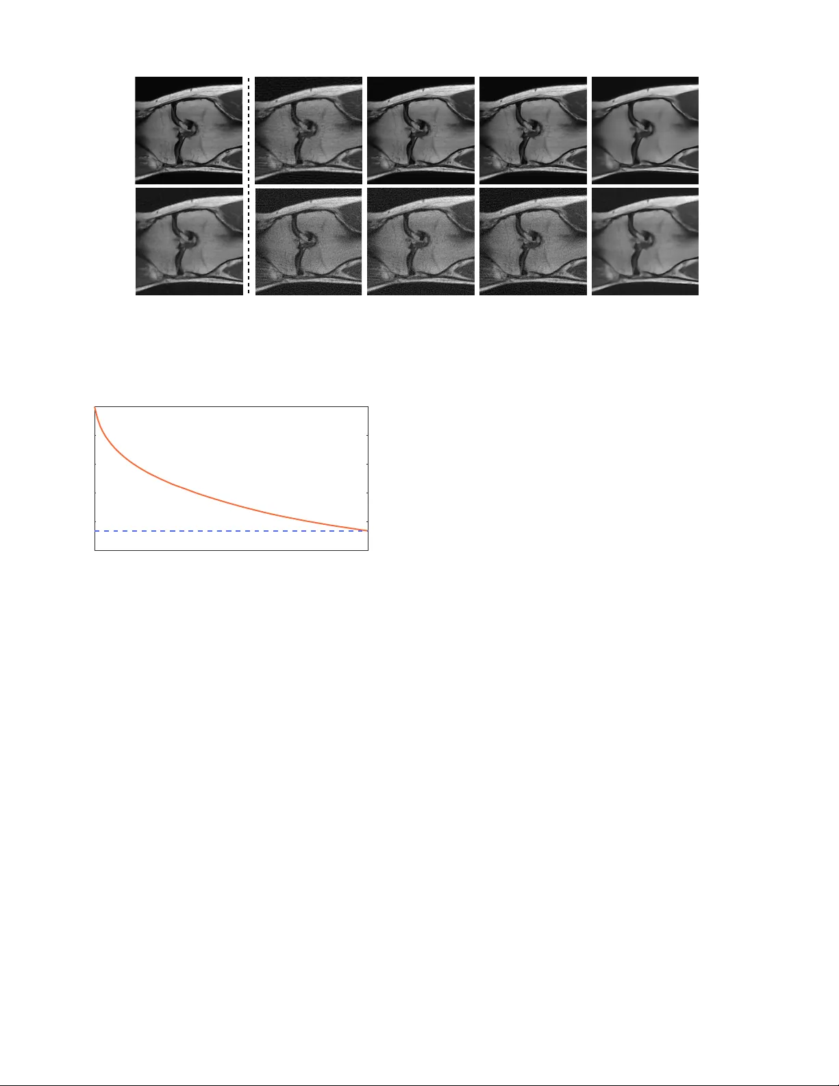
BLOCK COORDINA TE REGULARIZA TION BY DENOISING 1 Block Coordinate Re gularization by Denoising Y u Sun ∗ Student Member , IEEE , Jiaming Liu ∗ Student Member , IEEE , and Ulugbek S. Kamilov , Member , IEEE Abstract —W e consider the problem of estimating a vector fr om its noisy measurements using a prior speciﬁed only through a denoising function. Recent work on plug-and-play priors (PnP) and regularization-by-denoising (RED) has shown the state-of- the-art perf ormance of estimators under such priors in a range of imaging tasks. In this work, we develop a new block coor- dinate RED algorithm that decomposes a large-scale estimation problem into a sequence of updates over a small subset of the unknown variables. W e theoretically analyze the con vergence of the algorithm and discuss its relationship to the traditional proximal optimization. Our analysis complements and extends recent theoretical results for RED-based estimation methods. W e numerically validate our method using several denoiser priors, including those based on con volutional neural network (CNN) denoisers. I . I N T R O D U C T I O N Problems in volving estimation of an unknown vector x ∈ R n from a set of noisy measurements y ∈ R m are important in many areas, including computational imaging, machine learning, and compressiv e sensing. Consider the scenario in Fig. 1, where a vector x ∼ p x passes through the measurement channel p y | x to produce the measurement vector y . When the estimation problem is ill-posed, it becomes essential to include the prior p x in the estimation process. Ho wev er , in high- dimensional settings, it is difﬁcult to directly obtain the true prior p x for certain signals (such as natural images) and one is hence restricted to various indirect sources of prior information on x . This paper considers the cases where the prior information on x is speciﬁed only via a denoising function, D : R n → R n , designed for the remov al of additiv e white Gaussian noise (A WGN). There has been considerable recent interest in leveraging denoisers as priors for the reco very of x . One popular strategy , known as plug-and-play priors (PnP) [1], extends traditional proximal optimization [2] by replacing the proximal operator with a general off-the-shelf denoiser . It has been shown that the combination of proximal algorithms with advanced denoisers, such as BM3D [3] or DnCNN [4], leads to the state-of-the-art performance for v arious imaging problems [5]–[15]. A similar strategy has also been adopted in the context of a related This material is based upon work supported in part by NSF award CCF- 1813910 and by NVIDIA Corporation with the donation of the Titan Xp GPU for research. This paper was presented at the 2019 33th Annual Conference on Neural Information Processing Systems (NeurIPS). Y . Sun is with the Department of Computer Science & Engineering, W ashington Univ ersity in St. Louis, MO 63130, USA. J. Liu is with the Department of Electrical & Systems Engineering, W ashington Univ ersity in St. Louis, MO 63130, USA. U. S. Kamilov (email: kamilov@wustl.edu) is with the Department of Computer Science & Engineering and the Department of Electrical & Systems Engineering, W ashington Univ ersity in St. Louis, MO 63130, USA. ∗ indicates equal contribution p x ( x ) AAACCnicbVDLSsNAFL3xWesr1qWbYBHqpiRV0GXBjcsK9gFtCJPppB06MwkzE2kJ+QO/wa2u3Ylbf8Klf+L0sbCtBy73cM693MsJE0aVdt1va2Nza3tnt7BX3D84PDq2T0otFacSkyaOWSw7IVKEUUGammpGOokkiIeMtMPR3dRvPxGpaCwe9SQhPkcDQSOKkTZSYJeSIOuFPBvneWXeLwO77FbdGZx14i1IGRZoBPZPrx/jlBOhMUNKdT030X6GpKaYkbzYSxVJEB6hAekaKhAnys9mv+fOhVH6ThRLU0I7M/XvRoa4UhMemkmO9FCtelPxP6+b6ujWz6hIUk0Enh+KUubo2JkG4fSpJFiziSEIS2p+dfAQSYS1iWvpSshzk4m3msA6adWq3lW19nBdrtcW6RTgDM6hAh7cQB3uoQFNwDCGF3iFN+vZerc+rM/56Ia12DmFJVhfv3pGmzc= x 2 R n AAACD3icbVC7TsMwFHXKq5RXgYGBxaJCYqqSggRjJRbGguhDakJlu25r1XYi20FUUT6Cb2CFmQ2x8gmM/AlOm4G2HOlKR+fcq3vvwRFn2rjut1NYWV1b3yhulra2d3b3yvsHLR3GitAmCXmoOhhpypmkTcMMp51IUSQwp208vs789iNVmoXy3kwiGgg0lGzACDJW6pWPfCySpxT6TEJfIDPCOLlLH6xTcavuFHCZeDmpgByNXvnH74ckFlQawpHWXc+NTJAgZRjhNC35saYRImM0pF1LJRJUB8n0gRSeWqUPB6GyJQ2cqn8nEiS0nghsO7Mb9aKXif953dgMroKEySg2VJLZokHMoQlhlgbsM0WJ4RNLEFHM3grJCClEjM1sbgsWqc3EW0xgmbRqVe+8Wru9qNRreTpFcAxOwBnwwCWogxvQAE1AQApewCt4c56dd+fD+Zy1Fpx85hDMwfn6BeTJnQk= p y | x ( y | x ) AAACHHicbZDLSsNAFIYn9VbrLerSzWAV6qYkVdBlwY3LCvYCbQiT6aQdOpOEmYkYYl7Ah/AZ3OranbgVXPomTtosbOsPAx//OYdz5vciRqWyrG+jtLK6tr5R3qxsbe/s7pn7Bx0ZxgKTNg5ZKHoekoTRgLQVVYz0IkEQ9xjpepPrvN69J0LSMLhTSUQcjkYB9SlGSluueRK56cDjaZLBR5jDQ5bVFowz16xadWsquAx2AVVQqOWaP4NhiGNOAoUZkrJvW5FyUiQUxYxklUEsSYTwBI1IX2OAOJFOOv1NBk+1M4R+KPQLFJy6fydSxKVMuKc7OVJjuVjLzf9q/Vj5V05KgyhWJMCzRX7MoAphHg0cUkGwYokGhAXVt0I8RgJhpQOc2+LxTGdiLyawDJ1G3T6vN24vqs1GkU4ZHIFjUAM2uARNcANaoA0weAIv4BW8Gc/Gu/FhfM5aS0YxcwjmZHz9AlpSops= y 2 R m AAACD3icbVC7TsMwFHV4lvIKMDCwWFRITFVSkGCsxMJYEH1ITahs122t2k5kO0hRlI/gG1hhZkOsfAIjf4LbZqAtR7rS0Tn36t57cMyZNp737aysrq1vbJa2yts7u3v77sFhS0eJIrRJIh6pDkaaciZp0zDDaSdWFAnMaRuPbyZ++4kqzSL5YNKYhgINJRswgoyVeu5xgEWW5jBgEgYCmRHG2X3+KHpuxat6U8Bl4hekAgo0eu5P0I9IIqg0hCOtu74XmzBDyjDCaV4OEk1jRMZoSLuWSiSoDrPpAzk8s0ofDiJlSxo4Vf9OZEhonQpsOyc36kVvIv7ndRMzuA4zJuPEUElmiwYJhyaCkzRgnylKDE8tQUQxeyskI6QQMTazuS1Y5DYTfzGBZdKqVf2Lau3uslKvFemUwAk4BefAB1egDm5BAzQBATl4Aa/gzXl23p0P53PWuuIUM0dgDs7XL+TbnQk= unknown prior unknown vector known likelihood available meas. estimation algorithm MAP denoiser MMSE denoiser CNN denoiser A W GN denoiser s available denoiser D ( · ) AAACCXicbVDLSsNAFJ3UV62vVJduBotQNyWpgi4LunBZwT6gCWUynbRDZzJhZqKUkC/wG9zq2p249Stc+idO0yy09cCFwzn3cg8niBlV2nG+rNLa+sbmVnm7srO7t39gVw+7SiQSkw4WTMh+gBRhNCIdTTUj/VgSxANGesH0eu73HohUVET3ehYTn6NxREOKkTbS0K56HOmJCtObrO7hkdBnQ7vmNJwccJW4BamBAu2h/e2NBE44iTRmSKmB68TaT5HUFDOSVbxEkRjhKRqTgaER4kT5aR49g6dGGcFQSDORhrn6+yJFXKkZD8xmHnTZm4v/eYNEh1d+SqM40STCi0dhwqAWcN4DHFFJsGYzQxCW1GSFeIIkwtq09edLwDPTibvcwCrpNhvueaN5d1FrNYt2yuAYnIA6cMElaIFb0AYdgMEjeAYv4NV6st6sd+tjsVqyipsj8AfW5w/ws5pR b x = f D ( y ) AAACIXicbVDLSsNAFJ3UV62vqEs3g0VoNyWpgm6Egi5cVrAPaEqZTCbt0JkkzEzUEPINfoTf4FbX7sSduPJPnLZZ2NYDFw7n3Mu997gRo1JZ1pdRWFldW98obpa2tnd298z9g7YMY4FJC4csFF0XScJoQFqKKka6kSCIu4x03PHVxO/cEyFpGNypJCJ9joYB9SlGSksDs+o8UI+MkEodl6ePWQYvoT9IHY7USPrpdZZVJkaSVQdm2apZU8BlYuekDHI0B+aP44U45iRQmCEpe7YVqX6KhKKYkazkxJJECI/RkPQ0DRAnsp9OX8rgiVY86IdCV6DgVP07kSIuZcJd3Tk9ddGbiP95vVj5F/2UBlGsSIBni/yYQRXCST7Qo4JgxRJNEBZU3wrxCAmElU5xbovLM52JvZjAMmnXa/ZprX57Vm7U83SK4AgcgwqwwTlogBvQBC2AwRN4Aa/gzXg23o0P43PWWjDymUMwB+P7F67bpOY= AWGN denoisers denoisers Fig. 1. The estimation problem considered in this work. The vector x ∈ R n , with a prior p x ( x ) , passes through the measurement channel p y | x ( y | x ) to result in the measurements y ∈ R m . The estimation algorithm f D ( y ) does not hav e a direct access to the prior , but can rely on a denoising function D : R n → R n , speciﬁcally designed for the removal of additiv e white Gaussian noise (A WGN). W e propose block coordinate RED as a scalable algorithm for obtaining x gi ven y and D . class of algorithms kno wn as approximate message passing (AMP) [16]–[19]. Regularization-by-denoising (RED) [20], and the closely related deep mean-shift priors [21], represent an alternativ e, in which the denoiser is used to specify an explicit regularizer that has a simple gradient. More recent work has clariﬁed the existence of e xplicit RED regularizers [22], demonstrated its excellent performance on phase retrie v al [23], and further boosted its performance in combination with a deep image prior [24]. In short, the use of adv anced denoisers has prov en to be essential for achie ving the state-of-the-art results in many contexts. Howe ver , solving the corresponding estimation problem is still a signiﬁcant computational challenge, especially in the context of high-dimensional vectors x , typical in modern applications. In this work, we extend the current family of RED algo- rithms by introducing a new block coor dinate RED (BC-RED) algorithm. The algorithm relies on random partial updates on x , which mak es it scalable to vectors that w ould otherwise be prohibitiv ely large for direct processing. Additionally , as we shall see, the overall computational complexity of BC-RED can sometimes be lower than corresponding methods operating on the full vector . This behavior is consistent with the traditional coordinate descent methods that can outperform their full gradient counterparts by being able to better reuse local updates and take larger steps [25]–[29]. W e present two theoretical results related to BC-RED. W e ﬁrst theoretically characterize the conv ergence of the algorithm under a set of transparent assumptions on the data-ﬁdelity and the denoiser . Our analysis complements the recent theoretical analysis of full-gradient RED algorithms in [22] by considering block-coordinate updates and establishing the explicit w orst-case con vergence rate. Our second result establishes backward compatibility of BC-RED with the traditional proximal optimization. W e sho w that when the denoiser corresponds to a proximal operator , BC-RED can be interpreted as an approximate MAP estimator , whose approximation error can be made arbitrarily small. T o the best of our knowledge, this explicit link with proximal optimization is missing in the current literature on RED. BC- RED thus provides a ﬂe xible, scalable, and theoretically sound 2 BLOCK COORDINA TE REGULARIZA TION BY DENOISING algorithm applicable to a wide variety of large-scale estimation problems. W e demonstrate BC-RED on image recovery from linear measurements using sev eral denoising priors, including those based on conv olutional neural netw ork (CNN) denoisers. A preliminary version of this work has appeared in [30]. The current paper contains all the proofs, more detailed descriptions and additional simulations. I I . B AC K G R O U N D It is common to formulate the estimation in Figure 1 as an optimization problem b x = a rg min x ∈ R n f ( x ) with f ( x ) = g ( x ) + h ( x ) , (1) where g is the data-ﬁdelity term and h is the regularizer . For example, the maximum a posteriori probability (MAP) estimator is obtained by setting g ( x ) = − log ( p y | x ( y | x )) and h ( x ) = − log ( p x ( x )) , where p y | x is the likelihood that depends on y and p x is the prior . One of the most popular data-ﬁdelity terms is least-squares g ( x ) = 1 2 k y − Ax k 2 2 , which assumes a linear measurement model under A WGN. Similarly , one of the most popular re gularizers is based on a sparsity-promoting penalty h ( x ) = τ k D x k 1 , where D is a linear transform and τ > 0 is the re gularization parameter [31]–[34]. Many widely used regularizers, including the ones based on the ` 1 -norm, are nondifferentiable. Proximal algorithms [2], such as the proximal-gradient method (PGM) [35]–[38] and alternating direction method of multipliers (ADMM) [39]– [42], are a class of optimization methods that can circumv ent the need to dif ferentiate nonsmooth regularizers by using the proximal operator p rox µh ( z ) : = arg min x ∈ R n  1 2 k x − z k 2 2 + µh ( x )  , µ > 0 . (2) The observation that the proximal operator can be interpreted as the MAP denoiser for A WGN has prompted the de velopment of PnP [1], where the proximal operator p rox µh ( · ) , within ADMM or PGM, is replaced with a more general denoising function D ( · ) . Consider the following alternative to PnP that also relies on a denoising function [20], [21] x t ← x t − 1 − γ  ∇ g ( x t − 1 ) + H ( x t − 1 )  where H ( x ) : = τ ( x − D ( x )) , τ > 0 . (3) Under some conditions on the denoiser , it is possible to relate H ( · ) in (3) to some explicit regularization function h . For example, when the denoiser is locally homogeneous and has a symmetric Jacobian [20], [22], the operator H ( · ) corresponds to the gradient of the following function h ( x ) = τ 2 x T ( x − D ( x )) . (4) On the other hand, when the denoiser corresponds to the minimum mean squared error (MMSE) estimator D ( z ) = E [ x | z ] for the A WGN denoising problem [21], [22], z = x + e , with x ∼ p x ( x ) and e ∼ N ( 0 , σ 2 I ) , the operator H ( · ) corresponds to the gradient of h ( x ) = − τ σ 2 log ( p z ( x )) , (5) where p z ( x ) = ( p x ∗ p e )( x ) = Z R n p x ( z ) φ σ ( x − z ) d z , where φ σ is the Gaussian probability density function of variance σ 2 and ∗ denotes con volution. In this paper , we will use the term RED to denote all methods seeking the ﬁxed points of (3) . The k ey beneﬁts of the RED methods [20]–[24] are their explicit separation of the forward model from the prior , their ability to accommodate po werful denoisers (such as the ones based on CNNs) without dif ferentiating them, and their state-of-the-art performance on a number of imaging tasks. The next section further extends the scalability of RED by designing a new block coordinate RED algorithm. I I I . B L O C K C O O R D I N A T E R E D All the current RED algorithms operate on v ectors in R n . W e propose BC-RED, shown in Algorithm 1, to allow for partial randomized updates on x . Consider the decomposition of R n into b ≥ 1 subspaces R n = R n 1 × R n 2 × · · · × R n b with n = n 1 + n 2 + · · · + n b . For each i ∈ { 1 , . . . , b } , we deﬁne the matrix U i : R n i → R n that injects a vector in R n i into R n and its transpose U T i that extracts the i th block from a vector in R n . Then, for any x = ( x 1 , . . . , x b ) ∈ R n x = b X i =1 U i x i with x i = U T i x ∈ R n i , i = 1 , . . . , b (6) which is equiv alent to P b i =1 U i U T i = I . Note that (6) directly implies the norm preserv ation k x k 2 2 = k x 1 k 2 2 + · · · + k x b k 2 2 for any x ∈ R n . W e are interested in a block-coordinate algorithm that uses only a subset of operator outputs corresponding to coordinates in some block i ∈ { 1 , . . . , b } . Hence, for an operator G : R n → R n , we deﬁne the block-coordinate operator G i : R n → R n i as G i ( x ) : = [ G ( x )] i = U T i G ( x ) ∈ R n i , x ∈ R n . (7) W e now introduce the proposed BC-RED algorithm summarized in Algorithm 1. Note that when b = 1 , we have n = n 1 and U 1 = U T 1 = I . Hence, the theoretical analysis in this paper is also applicable to the full-gradient RED algorithm in (3). As with traditional coordinate descent methods (see [28] for a re vie w), BC-RED can be implemented using dif ferent block selection strategies. The strate gy adopted for our theoretical analysis selects block indices i k as i.i.d. random variables distributed uniformly over { 1 , . . . , b } . An alternativ e is to proceed in epochs of b consecutiv e iterations, where at the start of each epoch the set { 1 , . . . , b } is reshufﬂed, and i k is then selected consecutiv ely from this ordered set. W e numerically compare the conv ergence of both BC-RED variants in Section V. SUN, LIU, AND KAMILO V 3 Algorithm 1 Block Coordinate Regularization by Denoising (BC-RED) 1: input: initial value x 0 ∈ R n , parameter τ > 0 , and step-size γ > 0 . 2: f or k = 1 , 2 , 3 , . . . do 3: Choose an index i k ∈ { 1 , . . . , b } 4: x k ← x k − 1 − γ U i k G i k ( x k − 1 ) where G i ( x ) : = U T i G ( x ) with G ( x ) : = ∇ g ( x ) + τ ( x − D ( x )) . 5: end f or BC-RED updates its iterates one randomly picked block at a time using the output of G . When the algorithm conv erges, it con verges to the v ectors in the zero set of G G ( x ∗ ) = ∇ g ( x ∗ ) + τ ( x ∗ − D ( x ∗ )) = 0 ⇔ x ∗ ∈ zer ( G ) : = { x ∈ R n : G ( x ) = 0 } . (8) Consider the following two sets zer ( ∇ g ) : = { x ∈ R n : ∇ g ( x ) = 0 } and ﬁx ( D ) : = { x ∈ R n : x = D ( x ) } , (9) where zer ( ∇ g ) is the set of all critical points of the data- ﬁdelity and ﬁx ( D ) is the set of all ﬁxed points of the denoiser . Intuitiv ely , the ﬁxed points of D correspond to all the vectors that are not denoised, and therefore can be interpreted as v ectors that are noise-free according to the denoiser . Note that if x ∗ ∈ zer ( ∇ g ) ∩ ﬁx ( D ) , then G ( x ∗ ) = 0 and x ∗ is one of the solutions of BC-RED. Hence, any vector that is consistent with the data for a con ve x g and noiseless according to D is in the solution set. On the other hand, when zer ( ∇ g ) ∩ ﬁx ( D ) = ∅ , then x ∗ ∈ zer ( G ) corresponds to a tradeoff between the two sets, e xplicitly controlled via τ > 0 (see Fig. 8 in the supplement for an illustration). This explicit control is one of the key dif ferences between RED and PnP . BC-RED beneﬁts from considerable ﬂexibility compared to the full-gradient RED. Since each update is restricted to only one block of x , the algorithm is suitable for parallel implementations and can deal with problems where the vector x is distrib uted in space and in time. Howe ver , the maximal beneﬁt of BC-RED is achie ved when G i is ef ﬁcient to ev aluate. Fortunately , it was systematically shown in [43] that many operators—common in machine learning, image processing, and compressi ve sensing—admit coor dinate friendly updates. For a speciﬁc example, consider the least-squares data- ﬁdelity g and a block-wise denoiser D . Deﬁne the residual vector r ( x ) : = Ax − y and consider a single iteration of BC- RED that produces x + by updating the i th block of x . Then, the update direction and the residual update can be computed as G i ( x ) = A T i r ( x ) + τ ( x i − D ( x i )) and r ( x + ) = r ( x ) − γ A i G i ( x ) , (10) where A i ∈ R m × n i is a submatrix of A consisting of the columns corresponding to the i th block. In many problems of practical interest [43], the complexity of working with A i is roughly b times lo wer than with A . Also, many advanced denoisers can be ef fecti vely applied on image patches rather than on the full image [44]–[46]. Therefore, in such settings, the speed of b iterations of BC-RED is expected to be at least comparable to a single iteration of the full-gradient RED (see also Section E). I V . C O N V E R G E N C E A N A L Y S I S A N D C O M PA T I B I L I T Y W I T H P RO X I M A L O P T I M I Z AT I O N In this section, we present two theoretical results related to BC-RED. W e ﬁrst establish its con ver gence to an element of zer ( G ) and then discuss its compatibility with the theory of proximal optimization. A. F ixed P oint Con ver gence of BC-RED Our analysis requires three assumptions that together serve as suf ﬁcient conditions for con ver gence. Assumption 1. The operator G is such that zer ( G ) 6 = ∅ . Ther e is a ﬁnite number R 0 such that the distance of the initial x 0 ∈ R n to the farthest element of zer ( G ) is bounded, that is max x ∗ ∈ zer ( G ) k x 0 − x ∗ k 2 ≤ R 0 . This assumption is necessary to guarantee conv ergence and is related to the existence of the minimizers in the literature on traditional coordinate minimization [25]–[28]. The ne xt tw o assumptions rely on Lipschitz constants along directions speciﬁed by speciﬁc blocks. W e say that G i is block Lipschitz continuous with constant λ i > 0 if k G i ( x ) − G i ( y ) k 2 ≤ λ i k h i k 2 , where x = y + U i h i , y ∈ R n , h i ∈ R n i . (11) When λ i = 1 , we say that G i is block nonexpansive . Note that if an operator G is globally λ -Lipschitz continuous, then it is straightforward to see that each G i = U T i G is also block λ -Lipschitz continuous. Assumption 2. The function g is continuously differ entiable and con vex. Additionally , for each i ∈ { 1 , . . . , b } the block gradient ∇ i g is block Lipschitz continuous with constant L i > 0 . W e deﬁne the larg est bloc k Lipsc hitz constant as L max : = max { L 1 , . . . , L b } . Let L > 0 denote the global Lipschitz constant of ∇ g . W e always hav e L max ≤ L and, for some g , it may e ven happen that L max = L/b [28]. As we shall see, the largest possible step-size γ of BC-RED depends on L max , while that of the full-gradient RED on L . Hence, one natural advantage of BC- RED is that it can often take more aggressiv e steps compared to the full-gradient RED. Assumption 3. The denoiser D is such that each block denoiser D i is bloc k none xpansive. Since the proximal operator is nonexpansiv e [2], it auto- matically satisﬁes this assumption. W e re visit this scenario in a greater depth in Section IV -B . W e can now establish the following result for BC-RED. 4 BLOCK COORDINA TE REGULARIZA TION BY DENOISING Theorem 1. Run BC-RED for t ≥ 1 iterations with random i.i.d. bloc k selection under Assumptions 1-3 using a ﬁxed step- size 0 < γ ≤ 1 / ( L max + 2 τ ) . Then, we have E  min k ∈{ 1 ,...,t } k G ( x k − 1 ) k 2 2  ≤ E " 1 t t X k =1 k G ( x k − 1 ) k 2 2 # ≤ b ( L max + 2 τ ) γ t R 2 0 . (12) A proof of the theorem is provided in the supplement. Theorem 1 establishes the ﬁxed-point con ver gence of BC- RED in expectation to zer ( G ) with O (1 /t ) rate. The proof relies on the monotone operator theory [47], [48], widely used in the context of conv ex optimization [2], including in the uniﬁed analysis of various traditional coordinate descent algorithms [49], [50]. Note that the theorem does not assume the e xistence of any re gularizer h , which makes it applicable to denoisers beyond those characterized with explicit functions in (4) and (5). Since L max ≤ L , one important implication of Theorem 1, is that the worst-case con vergence rate (in e xpectation) of b iterations of BC-RED is better than that of a single iteration of the full-gradient RED (to see this, note that the full-gradient rate is obtained by setting b = 1 , L max = L , and remo ving the expectation in (12) ). This implies that in coor dinate friendly settings (as discussed at the end of Section III), the o verall computational complexity of BC-RED can be lo wer than that of the full-gradient RED. This gain is primarily due to two factors: (a) possibility to pick a larger step-size γ = 1 / ( L max + 2 τ ) ; (b) immediate reuse of each local block-update when computing the ne xt iterate (the full-gradient RED updates the full vector before computing the next iterate). In the special case of D ( x ) = x − (1 /τ ) ∇ h ( x ) , for some con vex function h , BC-RED reduces to the traditional coordinate descent method applied to (1) . Hence, under the assumptions of Theorem 1, one can rely on the analysis of traditional randomized coordinate descent methods in [28] to obtain E  f ( x t )  − f ∗ ≤ 2 b γ t R 2 0 (13) where f ∗ is the minimum value in (1) . A proof of (13) is provided in the supplement for completeness. Therefore, such denoisers lead to explicit con ve x RED regularizers and O (1 /t ) con ver gence of BC-RED in terms of the objecti ve. Howe ver , as discussed in Section IV -B , when the denoiser is a proximal operator of some con ve x h , BC-RED is not directly solving (1) , but rather its approximation. Finally , note that the analysis in Theorem 1 only provides sufﬁcient conditions for the con ver gence of BC-RED. As corroborated by our numerical studies in Section V, the actual con ver gence of BC-RED is more general and often holds beyond nonexpansiv e denoisers. One plausible explanation for this is that such denoisers are locally none xpansive o ver the set of input vectors used in testing. On the other hand, the recent techniques for spectral-normalization of CNNs [51]–[53] provide a con venient tool for building globally none xpansive neural denoisers that result in provable conv ergence of BC- RED. B. Con vergence for Pr oximal Operators One of the limitations of the current RED theory is in its limited backward compatibility with the theory of proximal optimization. For example, as discussed in [20] (see section “Can we mimic any prior?” ), the popular total v ariation (TV) denoiser [31] cannot be justiﬁed with the original RED regularization function (4) . In this section, we show that BC- RED (and hence also the full-gradient RED) can be used to solve (1) for any con vex, closed, and proper function h . W e do this by establishing a formal link between RED and the concept of Moreau smoothing, widely used in nonsmooth optimization [54]–[56]. In particular , we consider the following proximal-operator denoiser D ( z ) = pro x 1 τ h ( z ) = arg min x ∈ R n  1 2 k x − z k 2 2 + (1 /τ ) h ( x )  , (14) where τ > 0 , z ∈ R n , and h is a closed, proper , and conv ex function [2]. Since the proximal operator is nonexpansi ve, it is also block nonexpansi ve, which means that Assumption 3 is automatically satisﬁed. Our analysis, howev er , requires an additional assumption using the constant R 0 deﬁned in Assumption 1. Assumption 4. Ther e is a ﬁnite number G 0 that bounds the lar gest subgradient of h , that is max {k g ( x ) k 2 : g ( x ) ∈ ∂ h ( x ) , x ∈ B ( x 0 , R 0 ) } ≤ G 0 , wher e B ( x 0 , R 0 ) : = { x ∈ R n : k x − x 0 k 2 ≤ R 0 } denotes a ball of radius R 0 , center ed at x 0 . This assumption on boundedness of the subgradients holds for a large number of regularizers used in practice, including both TV and the ` 1 -norm penalties. W e can now establish the following result. Theorem 2. Run BC-RED for t ≥ 1 iterations with random i.i.d. block selection and the denoiser (14) under Assumptions 1- 4 using a ﬁxed step-size 0 < γ ≤ 1 / ( L max + 2 τ ) . Then, we have E  f ( x t )  − f ∗ ≤ 2 b γ t R 2 0 + G 2 0 2 τ , (15) wher e the function f is deﬁned in (1) and f ∗ is its minimum. The theorem is proved in the supplement. It establishes that BC-RED in expectation appr oximates the solution of (1) with an error bounded by ( G 2 0 / (2 τ )) . F or example, by setting τ = √ t and γ = 1 / ( L max + 2 √ t ) , one obtains the follo wing bound E  f ( x t )  − f ∗ ≤ 1 √ t  2 b ( L max + 2) R 2 0 + G 2 0  . (16) When h ( x ) = − log ( p x ( x )) , the proximal operator cor - responds to the MAP denoiser , and the solution of BC- RED corresponds to an appr oximate MAP estimator . This approximation can be made as precise as desired by considering larger values for the parameter τ > 0 . Note that this further justiﬁes the RED frame work by establishing that it can be used to compute a minimizer of any proper , closed, and conv ex SUN, LIU, AND KAMILO V 5 (but not necessarily differentiable) h . Therefore, our analysis strengthens RED by sho wing that it can accommodate a much larger class of e xplicit re gularization functions, be yond those characterized in (4) and (5). V . N U M E R I C A L V A L I DAT I O N There is a considerable recent interest in using adv anced priors in the context of image recovery from underdetermined ( m < n ) and noisy measurements. Recent work [20]–[24] suggests signiﬁcant performance improvements due to adv anced denoisers (such as BM3D [3] or DnCNN [4]) over traditional sparsity-driv en priors (such as TV [31]). Our goal is to complement these studies with se veral simulations validating our theoretical analysis and providing additional insights into BC-RED. The code for our implementation of BC-RED is av ailable through the follo wing link 1 . W e consider in verse problems of form y = Ax + e , where e ∈ R m is an A WGN vector and A ∈ R m × n is a matrix corresponding to either a sparse-view Radon transform, i.i.d. zero-mean Gaussian random matrix of variance 1 /m , or radially subsampled two-dimensional F ourier transform. Such matrices are commonly used in the context of computerized tomography (CT) [57], compressiv e sensing [33], [34], and magnetic resonance imaging (MRI) [58], respecti vely . In all simulations, we set the measurement ratio to be approximately m/n = 0 . 5 with A WGN corresponding to input signal-to- noise ratio (SNR) of 30 dB and 40 dB. The images used correspond to 10 images randomly selected from the NYU fastMRI dataset [59], resized to be 160 × 160 pixels (see Fig. 5 in the supplement). BC-RED is set to work with 16 blocks, each of size 40 × 40 pixels. The reconstruction quality is quantiﬁed using SNR averaged over all ten test images. In addition to well-studied denoisers, such as TV and BM3D, we design our own CNN denoiser denoted DnCNN ∗ , which is a simpliﬁed v ersion of the popular DnCNN denoiser (see Supplement D for details). This simpliﬁcation reduces the computational complexity of denoising, which is important when running many iterations of BC-RED. Additionally , it makes it easier to control the global Lipschitz constant of the CNN via spectral-normalization [52]. W e train DnCNN ∗ for the remov al of A WGN at four noise le vels corresponding to σ ∈ { 5 , 10 , 15 , 20 } . For each experiment, we select the denoiser achieving the highest SNR value. Note that the σ parameter of BM3D is also ﬁne-tuned for each experiment from the same set { 5 , 10 , 15 , 20 } . Theorem 1 establishes the con ver gence of BC-RED in expectation to an element of zer ( G ) . This is illustrated in Fig. 2 (left) for the Radon matrix with 30 dB noise and a none xpansiv e DnCNN ∗ denoiser (see also Fig. 6 in the supplement). The a verage value of k G ( x k ) k 2 2 / k G ( x 0 ) k 2 2 is plotted against the iteration number for the full-gradient RED and BC-RED, with b updates of BC-RED (each modifying a single block) represented as one iteration. W e numerically tested two block selection rules for BC-RED ( i.i.d. and epoch ) and observed that processing in randomized epochs leads to a faster con ver gence. For reference, the ﬁgure also plots the normalized 1 https://github .com/wustl- cig/bcred squared norm of the gradient mapping vectors produced by the traditional PGM with TV [60]. The shaded areas indicate the range of values taken o ver 10 runs corresponding to each test image. The results highlight the potential of BC-RED to enjoy a better con vergence rate compared to the full-gradient RED, with BC-RED (epoch) achieving the accuracy of 10 − 10 in 104 iterations, while the full-gradient RED achiev es the same accurac y in 190 iterations. Theorem 2 establishes that for proximal-operator denoisers, BC-RED computes an approximate solution to (1) with an accuracy controlled by the parameter τ . This is illustrated in Fig. 2 (right) for the Fourier matrix with 40 dB noise and the TV regularized least-squares problem. The av erage value of ( f ( x k ) − f ∗ ) / ( f ( x 0 ) − f ∗ ) is plotted against the iteration number for BC-RED with τ ∈ { 0 . 01 , 0 . 1 , 1 } . The optimal v alue f ∗ is obtained by running the traditional PGM until con vergence. As before, the ﬁgure groups b updates of BC-RED as a single iteration. The results are consistent with our theoretical analysis and show that as τ increases BC-RED provides an increasingly accurate solution to TV . On the other hand, since the range of possible values for the step-size γ depends on τ , the speed of con ver gence to f ∗ is also inﬂuenced by τ . The beneﬁts of the full-gradient RED algorithms ha ve been well discussed in prior work [20]–[24]. T able I summarizes the a verage SNR performance of BC-RED in comparison to the full-gradient RED for all three matrix types and se veral priors. Unlike the full-gradient RED, BC-RED is implemented using block-wise denoisers that work on image patches rather than the full images. W e empirically found that 40 pixel padding on the denoiser input is sufﬁcient for BC-RED to match the performance of the full-gradient RED. The table also includes the results for the traditional PGM with TV [60] and the widely-used end-to-end U-Net approach [61], [62]. The latter ﬁrst backprojects the measurements into the image domain and then denoises the result using U-Net [63]. The model was speciﬁcally trained end-to-end for the Radon matrix with 30 dB noise and applied as such to other measurement settings. All the algorithms were run until con vergence with hyperparameters optimized for SNR. The DnCNN ∗ denoiser in the table corresponds to the residual network with the Lipschitz constant of two (see Supplement F for details). The ov erall best SNR in the table is highlighted in bold-italic, while the best RED prior is highlighted in light-green. First, note the excellent agreement between BC-RED and the full- gradient RED. This close agreement between two methods is encouraging as BC-RED relies on block-wise denoising and our analysis does not establish uniqueness of the solution, yet, in practice, both methods seem to yield solutions of nearly identical quality . Second, note that BC-RED and RED provide excellent approximations to PGM-TV solutions. Third, note how (unlike U-Net) BC-RED and RED with DnCNN ∗ generalize to different measurement models. Finally . no prior seems to be universally good on all measurement settings, which indicates to the potential beneﬁt of tailoring speciﬁc priors to speciﬁc measurement models. Coordinate descent methods are known to be highly ben- eﬁcial in problems where both m and n are very lar ge, 6 BLOCK COORDINA TE REGULARIZA TION BY DENOISING 10 0 10 3 k 10 -7 10 0 f(x k )-f(x * ) ⌧ =1 AAAB/nicdVDLSgMxFM3UV62vqks3wSK4GibtlLYLoejGZQVrC+1QMmnahiaZIckIZSj4DW517U7c+isu/RPTh2BFD1w4nHMv994Txpxp43kfTmZtfWNzK7ud29nd2z/IHx7d6ShRhDZJxCPVDrGmnEnaNMxw2o4VxSLktBWOr2Z+654qzSJ5ayYxDQQeSjZgBBsrtbsGJ/ACol6+4Lk+8iu1GvRc5BUr5ZIlfhWhahki15ujAJZo9PKf3X5EEkGlIRxr3UFebIIUK8MIp9NcN9E0xmSMh7RjqcSC6iCd3zuFZ1bpw0GkbEkD5+rPiRQLrScitJ0Cm5H+7c3Ev7xOYgbVIGUyTgyVZLFokHBoIjh7HvaZosTwiSWYKGZvhWSEFSbGRrSyJRRTm8n34/B/cld0Uckt3viF+uUynSw4AafgHCBQAXVwDRqgCQjg4BE8gWfnwXlxXp23RWvGWc4cgxU471/975YH ⌧ = 10  2 AAACBHicdVC7TgJBFJ3FF+ILtbSZSExs3MyyIEthQrSxxETABBYyOwwwYfaRmVkTsqH1G2y1tjO2/oelf+IsYCJGT3KTk3Puzb33eBFnUiH0YWRWVtfWN7Kbua3tnd29/P5BU4axILRBQh6KOw9LyllAG4opTu8iQbHvcdryxlep37qnQrIwuFWTiLo+HgZswAhWWup2FI7hBbRQNzkrTnv5AjKR7aBqBSLTLlcdu6zJuVMqIQdaJpqhABao9/KfnX5IYp8GinAsZdtCkXITLBQjnE5znVjSCJMxHtK2pgH2qXST2dVTeKKVPhyEQleg4Ez9OZFgX8qJ7+lOH6uR/O2l4l9eO1YDx01YEMWKBmS+aBBzqEKYRgD7TFCi+EQTTATTt0IywgITpYNa2uL5aSbfj8P/SbNoWrZZvCkVapeLdLLgCByDU2CBCqiBa1AHDUCAAI/gCTwbD8aL8Wq8zVszxmLmECzBeP8C+nyYMw== ⌧ = 10  1 AAACBHicdVC7SgNBFJ2NrxhfUUubwSDYuMxmE90UQtDGMoJ5QLIJs5NJMmT2wcysEJa0foOt1nZi639Y+ifOJhGM6IELh3Pu5d57vIgzqRD6MDIrq2vrG9nN3Nb2zu5efv+gIcNYEFonIQ9Fy8OSchbQumKK01YkKPY9Tpve+Dr1m/dUSBYGd2oSUdfHw4ANGMFKS92OwjG8hBbqJmfWtJcvINNBJcspQ2QW7YpVsTVBjl0unUPLRDMUwAK1Xv6z0w9J7NNAEY6lbFsoUm6ChWKE02muE0saYTLGQ9rWNMA+lW4yu3oKT7TSh4NQ6AoUnKk/JxLsSznxPd3pYzWSv71U/Mtrx2rguAkLoljRgMwXDWIOVQjTCGCfCUoUn2iCiWD6VkhGWGCidFBLWzw/zeT7cfg/aRRNyzaLt6VC9WqRThYcgWNwCixwAargBtRAHRAgwCN4As/Gg/FivBpv89aMsZg5BEsw3r8A6G+YJw== iteration 0 10 3 ( f ( x k )  f ⇤ ) / ( f ( x 0 )  f ⇤ ) AAACG3icbVDLTgIxFO3gC/GFunTTSEzARJxBE10S3bjERB4JDKRTOtDQdiZtx0gmfIAf4Te41bU749aFS//EApMo4EmanJxzbu7t8UJGlbbtLyu1tLyyupZez2xsbm3vZHf3aiqIJCZVHLBANjykCKOCVDXVjDRCSRD3GKl7g+uxX78nUtFA3OlhSFyOeoL6FCNtpE42l/fzLY/HD6P2oHDit48Lp7+KPVVMyi7aE8BF4iQkBxJUOtnvVjfAESdCY4aUajp2qN0YSU0xI6NMK1IkRHiAeqRpqECcKDeefGYEj4zShX4gzRMaTtS/EzHiSg25Z5Ic6b6a98bif14z0v6lG1MRRpoIPF3kRwzqAI6bgV0qCdZsaAjCkppbIe4jibA2/c1s8fjIdOLMN7BIaqWic1Ys3Z7nyldJO2lwAA5BHjjgApTBDaiAKsDgETyDF/BqPVlv1rv1MY2mrGRmH8zA+vwBT3OfpQ== 10 0 10 − 7 Fourier (40 dB) 0 250 500 iteration 10 -14 10 -7 10 0 (x-Px)/(x0-Px0) k G ( x k ) k 2 2 / k G ( x 0 ) k 2 2 AAACM3icbVDLSsNAFJ34rPUVdelmsAh1U5MqKLgputBlBfuApi2T6aQdOpOEmYlY0nyMH+E3uNWluFLc+g9O2yzs48CFwzn3cu89bsioVJb1YSwtr6yurWc2sptb2zu75t5+VQaRwKSCAxaIuoskYdQnFUUVI/VQEMRdRmpu/2bk1x6JkDTwH9QgJE2Ouj71KEZKS23zyhk6HKme9OLbJO+4PH5KWv0TZ9gutorwFC6yrdRumzmrYI0B54mdkhxIUW6bX04nwBEnvsIMSdmwrVA1YyQUxYwkWSeSJES4j7qkoamPOJHNePxkAo+10oFeIHT5Co7V/xMx4lIOuKs7xxfPeiNxkdeIlHfZjKkfRor4eLLIixhUARwlBjtUEKzYQBOEBdW3QtxDAmGlc53a4vJEZ2LPJjBPqsWCfVYo3p/nStdpOhlwCI5AHtjgApTAHSiDCsDgGbyCN/BuvBifxrfxM2ldMtKZAzAF4/cPEZKrDw== iteration 0 500 10 − 14 10 0 Radon (30 dB) PGM ! RED ! BC-RED (i.i.d.) ! BC-RED (epoch) ⌧ =0 . 01 AAAB8nicdVDLSgMxFM3UV62vqks3wSK4GjLjaLsRim5cVrAPaEvJpGkbmskMyR2hlH6GGxeKuPVr3Pk3ZtoKKnogcHLOvdx7T5hIYYCQDye3srq2vpHfLGxt7+zuFfcPGiZONeN1FstYt0JquBSK10GA5K1EcxqFkjfD8XXmN++5NiJWdzBJeDeiQyUGglGwUrsDNMWXmLjE6xVLxC0HlaDs2793QfxzkhnlgBAfey6Zo4SWqPWK751+zNKIK2CSGtP2SALdKdUgmOSzQic1PKFsTIe8bamiETfd6XzlGT6xSh8PYm2fAjxXv3dMaWTMJAptZURhZH57mfiX105hUOlOhUpS4IotBg1SiSHG2f24LzRnICeWUKaF3RWzEdWUgU2pYEP4uhT/Txq+6525/m1Qql4t48ijI3SMTpGHyqiKblAN1RFDMXpAT+jZAefReXFeF6U5Z9lziH7AefsEaWKQCQ== ⌧ =0 . 001 AAAB83icdVDLSgMxFM34rPVVdekmWARXQ1JrRxdC0Y3LCvYBnaFk0kwbmnmQh1BKf8ONC0Xc+jPu/BszbQUVPRA4nHMu9+aEmeBKI/ThLC2vrK6tFzaKm1vbO7ulvf2WSo2krElTkcpOSBQTPGFNzbVgnUwyEoeCtcPRde6375lUPE3u9DhjQUwGCY84JdpKvq+JgZcQuQjhXqmMXIwvqt6ZFaoI1WqeJR6qYYwhtpEcZbBAo1d69/spNTFLNBVEqS5GmQ4mRGpOBZsWfaNYRuiIDFjX0oTETAWT2c1TeGyVPoxSaV+i4Uz9PjEhsVLjOLTJmOih+u3l4l9e1+joPJjwJDOaJXS+KDIC6hTmBcA+l4xqMbaEUMntrZAOiSRU25qKtoSvn8L/Savi4lO3clst168WdRTAITgCJwADD9TBDWiAJqAgAw/gCTw7xnl0XpzXeXTJWcwcgB9w3j4B46yQSg== Fig. 2. Left : Illustration of the con ver gence of BC-RED under a nonexpansi ve DnCNN ∗ prior . A verage normalized distance to zer ( G ) is plotted against the iteration number with the shaded areas representing the range of values attained over all test images. Right : Illustration of the inﬂuence of the parameter τ > 0 for solving TV regularized least-squares problem using BC-RED. As τ increases, BC-RED provides an increasingly accurate approximation to the TV optimization problem. T ABLE I A V E R AG E S N R S O B TAI N E D F O R D I FF E R EN T M E A S U RE M E N T M A T R IC E S A N D I M AG E P R I O R S . Methods Radon Random Fourier 30 dB 40 dB 30 dB 40 dB 30 dB 40 dB PGM (TV) 20.66 24.40 26.07 28.42 28.74 29.99 U-Net 21.90 21.72 16.37 16.40 22.11 22.11 RED (TV) 20.79 24.46 25.64 28.30 28.67 29.97 BC-RED (TV) 20.78 24.42 25.70 28.39 28.71 29.99 RED (BM3D) 21.55 25.24 26.46 27.82 28.89 29.79 BC-RED (BM3D) 21.56 25.16 26.50 27.88 28.85 29.80 RED (DnCNN ∗ ) 20.89 24.38 26.53 28.05 29.33 30.32 BC-RED (DnCNN ∗ ) 20.88 24.42 26.60 28.12 29.40 30.39 Fig. 3. Recovery of a 8292 × 8364 pixel galaxy image degraded by a spatially variant blur and a high-amount of A WGN. The efﬁcac y of BC-RED is due to the natural sparsity in this lar ge-scale problem, with all of the information contained in a small part of the full image. but each measurement depends only on a small subset of the unknowns [64]. Fig. 3 demonstrates BC-RED in such large-scale setting by adopting the experimental setup from a recent work [65] (see also Fig. 10 in the supplement). Speciﬁcally , we consider the recovery of a 8292 × 8364 pixel galaxy image degraded by 597 known point spread functions (PSFs) corresponding to different spatial locations. The natural sparsity of the problem makes it ideal for BC- RED, which is implemented to update 41 × 41 pixel blocks in a randomized fashion by only picking areas containing galaxies. The computational complexity of BC-RED is further reduced by considering a simpler variant of DnCNN ∗ that has only four con volutional layers (see Fig. 4 in the supplement). F or comparison, we additionally show the result obtained by using the low-rank recovery method from [65] with all the parameters kept at the v alues set by the authors. Note that our intent here is not to justify DnCNN ∗ as a prior for image deblurring, but to demonstrate that BC-RED can indeed be applied to a realistic, nontrivial image recov ery task on a lar ge image. V I . C O N C L U S I O N A N D F U T U R E W O R K Coordinate descent methods ha ve become increasingly im- portant in optimization for solving large-scale problems arising in data analysis. W e ha ve introduced BC-RED as a coordinate descent extension to the current family of RED algorithms and theoretically analyzed its conv ergence. Preliminary experiments suggest that BC-RED can be an effecti ve tool in large- scale estimation problems arising in image recov ery . More experiments are certainly needed to better asses the promise of this approach in various estimation tasks. For future work, we would like to explore accelerated and asynchronous variants of BC-RED to further enhance its performance in parallel settings. A P P E N D I X W e adopt the monotone operator theory [47], [48] for a uniﬁed analysis of BC-RED. In Supplement A, we prove SUN, LIU, AND KAMILO V 7 the con ver gence of BC-RED to an element of zer ( G ) . In Supplement A, we prove that for proximal-operator denoisers, BC-RED con ver ges to an approximate solution of (1) . For completeness, in Supplement A, we discuss the well-known con ver gence results for traditional coordinate descent [25]–[29]. In Supplement A, we provide the background material used in Supplement A and Supplement A, expressed in a form con venient for block-coordinate analysis. In Supplement D, we provide additional technical details omitted from the main paper due to space, such as the details on computational complexity and CNN architectures. In Supplement G, we present additional simulations that were also omitted from the main paper due to space. A ﬁxed-point conv ergence of averaged operators is well- known under the name of Krasnosel’ skii-Mann theorem (see Section 5.2 in [47]) and was recently applied to the analysis of PnP [13] and se veral full-gradient RED algorithms in [22]. Our analysis here e xtends these results to the block-coordinate setting and provides explicit worst-case con vergence rates for BC-RED. W e consider the following operators G i = ∇ i g + H i with H i = τ U T i ( I − D ) . and proceed in sev eral steps. (a) Since ∇ i g is block L i -Lipschitz continuous, it is also block L max -Lipschitz continuous. Hence, we know from Proposition 7 in Supplement C that it is block (1 /L max ) - cocoerciv e. Then from Proposition 4 in Supplement B, we kno w that the operator ( U T i − (2 /L max ) ∇ i g ) is block nonexpansi ve. (b) From the deﬁnition of H i and the fact that D i is block nonexpansi ve, we know that ( U T i − (1 /τ ) H i ) = D i is block none xpansiv e. (c) From Proposition 1 in Supplement A, we know that a con ve x combination of block none xpansiv e operators is also block nonexpansiv e, hence we conclude that U T i − 2 L max + 2 τ G i =  2 L max + 2 τ · L max 2   U T i − 2 L max ∇ i g  +  2 L max + 2 τ · 2 τ 2   U T i − 1 τ H i  , is block nonexpansiv e. Then from Proposition 4 in Supplement B, we know that G i is block 1 / ( L max + 2 τ ) - cocoerciv e. (d) Consider any x ∗ ∈ zer ( G ) , an index i ∈ { 1 , . . . , b } picked uniformly at random, and a single iteration of BC-RED x + = x − γ U i G i x . Deﬁne a vector h i : = U T i ( x − x ∗ ) ∈ R n i . W e then have k x + − x ∗ k 2 = k x − x ∗ − γ U i G i x k 2 = k x − x ∗ k 2 − 2 γ ( U i G i x ) T ( x − x ∗ ) + γ 2 k G i x k 2 = k x − x ∗ k 2 − 2 γ ( G i x − G i x ∗ ) T h i + γ 2 k G i x k 2 ≤k x − x ∗ k 2 − 2 γ − ( L max + 2 τ ) γ 2 L max + 2 τ k G i x k 2 ≤k x − x ∗ k 2 − γ L max + 2 τ k G i x k 2 , (17) where in the third line we used G i x ∗ = U T i G x ∗ = 0 , in the fourth line the block cocoercivity of G i , and in the last line the fact that 0 < γ ≤ 1 / ( L max + 2 τ ) . (e) By taking a conditional expectation on both sides and rearranging the terms, we obtain γ L max + 2 τ E  k G i x k 2 | x  = γ b ( L max + 2 τ ) b X i =1 k G i x k 2 = γ b ( L max + 2 τ ) k G x k 2 ≤ E  k x − x ∗ k 2 − k x + − x ∗ k 2 | x  (f) Hence by averaging over t ≥ 1 iterations and taking the total e xpectation E " 1 t t X k =1 k G x k − 1 k 2 # ≤ 1 t  b ( L max + 2 τ ) γ k x 0 − x ∗ k 2  ≤ 1 t  b ( L max + 2 τ ) γ R 2 0  . (18) The last inequality directly leads to the result. Remark . Eq. (17) implies that, under Assumptions 1-3, the iterates of BC-RED satisfy k x t − x ∗ k ≤ k x t − 1 − x ∗ k ≤ · · · ≤ k x 0 − x ∗ k ≤ R 0 , (19) which means that the distance of the iterates of BC-RED to zer ( G ) is nonincreasing. Remark . Suppose we are solving a coor dinate friendly pr oblem [43], in which the cost of the full gradient update is b times the cost of block update. Consider the step-size γ = 1 / ( L + 2 τ ) where L is the global Lipschitz constant of the gradient method. A similar analysis as above would yield the follo wing con vergence rate for the gradient method 1 t t X k =1 k G x k − 1 k 2 ≤ ( L + 2 τ ) 2 R 2 0 t Now , consider the step-size γ = 1 / ( L max + 2 τ ) and suppose that we run ( t · b ) updates of BC-RED with t ≥ 1 . Then, we hav e that E " 1 tb tb X k =1 k G x k − 1 k 2 # ≤ ( L max + 2 τ ) 2 R 2 0 t . Since L max ≤ L ≤ bL max , where the upper bound can sometimes be tight, we conclude that the e xpected complexity of the block-coordinate algorithm is lower compared to the full algorithm. 8 BLOCK COORDINA TE REGULARIZA TION BY DENOISING The concept of Moreau smoothing is well-known and has been e xtensiv ely used in other contexts (see for example [56]). Our contrib ution is to formally connect the concept to RED- based algorithms, which leads to its novel justiﬁcation as an approximate MAP estimator . The basic revie w of relev ant concepts from proximal optimization is given in Supplement D. For τ > 0 , we consider the Moreau env elope of h h (1 /τ ) ( x ) : = min z ∈ R n  1 2 k z − x k 2 + (1 /τ ) h ( z )  . From Proposition 9 in Supplement D we kno w that 0 ≤ h ( x ) − τ h (1 /τ ) ( x ) ≤ G 0 2 τ (20) and from Proposition 8 in Supplement D, we know that τ ∇ h (1 /τ ) ( x ) = τ ( x − pro x (1 /τ ) h ( x )) . (21) Hence, we can express the function f as follo ws f ( x ) = g ( x ) + h ( x ) = ( g ( x ) + τ h (1 /τ ) ( x )) + ( h ( x ) − τ h (1 /τ ) ( x )) = f (1 /τ ) ( x ) + ( h ( x ) − τ h (1 /τ ) ( x )) , where f (1 /τ ) : = g + τ h (1 /τ ) . From eq. (21) , we conclude that a single iteration of BC-RED x + = x − γ U i G i x with G i = U T i ( ∇ g ( x ) + τ ∇ h (1 /τ ) ( x )) is performing a block-coordinate descent on the function f (1 /τ ) . From eq. (20) and the conv exity of the Moreau env elope, we hav e f ∗ (1 /τ ) = f (1 /τ ) ( x ∗ ) ≤ f (1 /τ ) ( x ) ≤ f ( x ) , x ∈ R n , x ∗ ∈ zer ( G ) . Hence, there exists a ﬁnite f ∗ such that f ( x ) ≥ f ∗ with f ∗ (1 /τ ) ≤ f ∗ . Consider the iteration t ≥ 1 of BC-RED, then we ha ve that E [ f ( x t )] − f ∗ ≤ E [ f ( x t )] − f ∗ (1 /τ ) = ( E [ f (1 /τ ) ( x t )] − f ∗ (1 /τ ) ) + E [( h ( x t ) − τ h (1 /τ ) ( x t )]) ≤ 2 b γ t R 2 0 + G 2 0 2 τ , where we applied (13) , which is further discussed in Supple- ment A. The proof of eq. (16) is directly obtained by setting τ = √ t , γ = L max + 2 √ t , and noting that t ≥ √ t , for all t ≥ 1 . The following analysis has been adopted from [28]. W e include it here for completeness. Consider the following denoiser D ( x ) = x − 1 τ ∇ h ( x ) , τ > 0 , x ∈ R n , and the following function f ( x ) = g ( x ) + h ( x ) where g and h are both con ve x and continuously differentiable. For this denoiser , we have that G ( x ) = ∇ g ( x ) + τ ( x − D ( x )) = ∇ g ( x ) + ∇ h ( x ) = ∇ f ( x ) . Therefore, in this case, BC-RED is minimizing a conv ex and smooth function f , which means that any x ∗ ∈ zer ( G ) is a global minimizer of f . Additionally , due to Proposition 2 in Supplement A and Proposition 7 in Supplement C, we hav e D i is block nonexpansiv e ⇔ ∇ i h is block 2 τ -Lipschitz continuous . (22) Hence, for such denoisers, Assumption 3 is equiv alent to the 2 τ -Lipschitz smoothness of block gradients ∇ i h . T o prove eq. 13, we consider the follo wing iteration x + = x − U i G i x with G i = ∇ i f = ∇ i g + ∇ i h, which under our assumptions is a special case of the setting for Theorem 1. (a) From the block Lipscthiz continuity of f , we conclude that f ( x + ) ≤ f ( x ) + ∇ f ( x ) T ( x + − x ) + ( L max + 2 τ ) 2 k x + − x k 2 = f ( x ) − γ k∇ i f ( x ) k 2 + γ 2 ( L max + 2 τ ) 2 k∇ i f ( x ) k 2 ≤ f ( x ) − γ 2 k∇ i f ( x ) k 2 , where the last inequality comes from the fact that γ ≤ 1 / ( L max + 2 τ ) . (b) For all t ≥ 1 , deﬁne ϕ t : = E  f ( x t )  − f ( x ∗ ) . Then from (a), we can conclude that ϕ t ≤ ϕ t − 1 − γ 2 b E  k∇ f ( x t − 1 ) k 2  ≤ ϕ t − 1 − γ 2 b E  k∇ f ( x t − 1 ) k  2 , (23) where in the last inequality we used the Jensen’ s inequality , and the fact that E  k∇ i f ( x t − 1 ) k 2  = E  E  k∇ i f ( x t − 1 ) k 2 | x t − 1  = E " 1 b b X i =1 k∇ i f ( x t ) k 2 # = 1 b E  k∇ f ( x t − 1 ) k 2  . (24) (c) From con vexity , we kno w that ϕ t = E  f ( x t )  − f ( x ∗ ) ≤ E  ∇ f ( x t ) T ( x t − x ∗ )  ≤ E  k∇ f ( x t ) kk x t − x ∗ k  ≤ R 0 · E  k∇ f ( x t ) k  , (25) where in the last inequality , we used eq. (19) . This combined with the result of (b) implies that ϕ t ≤ ϕ t − 1 − γ 2 b ϕ 2 t − 1 R 2 0 . (d) Note that from (c), we can obtain 1 ϕ t − 1 ϕ t − 1 = ϕ t − 1 − ϕ t ϕ t ϕ t − 1 ≥ ϕ t − 1 − ϕ t ϕ 2 t − 1 ≥ γ 2 bR 2 0 . SUN, LIU, AND KAMILO V 9 By iterating this inequality , we get the ﬁnal result 1 ϕ t ≥ 1 ϕ 0 + γ t 2 b k x 0 − x ∗ k 2 ≥ γ t 2 bR 2 0 ⇒ ϕ t ≤ 2 b γ t R 2 0 . The results in this section are well-kno wn in the optimization literature and can be found in dif ferent forms in standard text- books [47], [55], [66], [67]. For completeness, we summarize the k ey results useful for our analysis by restating them in a block-coordinate form. A. Pr operties of Bloc k-Coor dinate Oper ators Most of the concepts in this part come from the tradi- tional monotone operator theory [47], [48] adapted for block- coordinate operators. Deﬁnition 1. W e deﬁne the block-coordinate operator T i : R n → R n i of T : R n → R n as T i x : = [ T x ] i = U T i T x ∈ R n i , x ∈ R n . The operator T i applies T to its input vector and then e xtracts the subset of outputs corresponding to the coor dinates in the block i ∈ { 1 , . . . , b } . Remark . When b = 1 , we hav e that n = n 1 and U 1 = U T 1 = I . Then, all the properties in this section reduce to their standard counterparts from the monotone operator theory in R n . In such settings, we simply drop the word block from the name of the property . Deﬁnition 2. T i is block Lipschitz continuous with constant λ i > 0 if k T i x − T i y k ≤ λ i k h i k , x = y + U i h i , y ∈ R n , h i ∈ R n i . When λ i = 1 , we say that T i is block nonexpansiv e . Deﬁnition 3. An operator T i is block cocoerci ve with constant β i > 0 if ( T i x − T i y ) T h i ≥ β i k T i x − T i y k 2 , x = y + U i h i , y ∈ R n , h i ∈ R n i . When β i = 1 , we say that T i is block ﬁrmly nonexpansi ve . The follo wing propositions are conclusions deri ved from the deﬁnition of above. Proposition 1. Let T ij : R n → R n i for j ∈ J be a set of block nonexpansive oper ators. Then, their conve x combination T i : = X j ∈ J θ j T ij , with θ j > 0 and X j ∈ J θ j = 1 , is none xpansive. Pr oof. By using the triangular inequality and the deﬁnition of block none xpansiv eness, we obtain k T i x − T i y k ≤ X j ∈ J θ j k T ij x − T ij y k ≤   X j ∈ J θ j   k h i k = k h i k , for all y ∈ R n and h i ∈ R n i where x = y + U i h i . Proposition 2. Consider R i = U T i − T i wher e T i : R n → R n i . T i is bloc k none xpansive ⇔ R i is (1 / 2) -bloc k cocoer cive. Pr oof. First suppose that R i is 1 / 2 block cocoercive. Let x = y + U i h i for all y ∈ R n and h i ∈ R n i . W e then have 1 2 k R i x − R i y k 2 ≤ ( R i x − R i y ) T h i = k h i k 2 − ( T i x − T i y ) T h i . W e also ha ve that 1 2 k R i x − R i y k 2 = 1 2 k h i k 2 − ( T i x − T i y ) T h i + 1 2 k T i x − T i y k 2 . By combining these two and simplifying the expression, we obtain that k T i x − T i y k ≤ k h i k . The con verse can be proved by following this logic in rev erse. B. Block A veraged Operators It is well kno wn that the iteration of a nonexpansi ve operator does not necessarily con ver ge. T o see this consider a nonexpansi ve operator T = − I , where I is identity . Ho wev er , it is also well kno wn that the con vergence can be established for a veraged operators. Deﬁnition 4. F or a constant α ∈ (0 , 1) , we say that the operator T is α -av eraged , if ther e exists a nonexpansive operator N such that T = (1 − α ) I + α N . Deﬁnition 5. F or a constant α ∈ (0 , 1) , we say that T i : R n → R n i is block α -av eraged , if there exists a block nonexpansive operator N i such that T i = (1 − α ) U T i + α N i . Remark . It is clear that if T is α -av eraged, then T i = U T i T is block α -averaged. The follo wing characterization is often con venient. Proposition 3. F or a block nonexpansive operator T i , a constant α ∈ (0 , 1) , and the operator R i : = U T i − T i , the following ar e equivalent (a) T i is bloc k α -aver aged (b) (1 − 1 /α ) U T i + (1 /α ) T i is bloc k none xpansive (c) k T i x − T i y k 2 ≤ k h i k 2 −  1 − α α  k R i x − R i y k 2 , x = y + U i h i , y ∈ R n , h i ∈ R n i Pr oof. The equiv alence of (a) and (b) is clear from the deﬁnition. T o establish the equi v alence with (c), consider an operator N i and T i = (1 − α ) U T i + α N i . Note that R i = U T i − T i = α ( U T i − N i ) . Then, for all y ∈ R n and h i ∈ R n i , with x = y + U i h i , we hav e that k T i x − T i y k 2 = k (1 − α ) h i + α ( N i x − N i y ) k 2 = (1 − α ) k h i k 2 + α k N i x − N i y k 2 − α (1 − α ) k h i − ( N i x − N i y ) k 2 = (1 − α ) k h i k 2 + α k N i x − N i y k 2 −  1 − α α  k R i x − R i y k 2 , (26) 10 BLOCK COORDINA TE REGULARIZA TION BY DENOISING where we used the fact that k (1 − α ) x + α y k 2 = (1 − α ) k x k 2 + α k y k 2 − α (1 − α ) k x − y k 2 , where θ ∈ R and x , y ∈ R n . Consider also k h i k 2 −  1 − α α  k R i x − R i y k 2 = (1 − α ) k h i k 2 + α k h i k 2 −  1 − α α  k R i x − R i y k 2 . (27) It is clear that we have (26) ≤ (27) ⇔ N i is block nonexpansiv e ⇔ T i is block α -averaged , (28) where for the last equiv alence, we used the deﬁnition of block av eragedness. Proposition 4. Consider a block-coor dinate operator T i = U T i T with T : R n → R n . Let x = y + U i h with x ∈ R n , h i ∈ R n i and consider β i > 0 . Then, the following ar e equivalent (a) T i is bloc k β i -cocoer cive (b) β i T i is bloc k ﬁrmly nonexpansive (c) U T i − β i T i is bloc k ﬁrmly nonexpansive. (d) β i T i is bloc k (1 / 2) -aver aged. (e) U T i − 2 β i T i is bloc k none xpansive. Pr oof. The equiv alence between (a) and (b) is readily observed by deﬁning P i : = β i T i and noting that ( P i x − P i y ) T h i = β i ( T i x − T i y ) T h i and k P i x − P i y k 2 = β 2 i k T i x − T i y k . (29) Deﬁne R i : = U T i − P i and suppose (b) is true, then ( R i x − R i y ) T h i = k h i k 2 − ( P i x − P i y ) T h i = k R i x − R i y k 2 + ( P i x − P i y ) T h i − k P i x − P i y k 2 ≥ k R i x − R i y k 2 . By repeating the same argument for P i = U T i − R i , we establish the full equiv alence between (b) and (c). The full equiv alence of (b) and (d) can be established by observing that 2 k P i x − P i y k 2 ≤ 2( P i x − P i y ) T h i ⇔ k P i x − P i y k 2 ≤ 2( P i x − P i y ) T h i − k P i x − P i y k 2 = k h i k 2 − ( k h i k 2 − 2( P i x − P i y ) T h i + k P i x − P i y k 2 ) = k h i k 2 − k R i x − R i y k 2 . T o show the equivalence with (e), ﬁrst suppose that N i : = U T i − 2 P i is block nonexpansi ve, then P i = 1 2 ( U T i + ( − N i )) is block 1 / 2 -av eraged, which means that it is block ﬁrmly nonexpansiv e. On the other hand, if P i is block ﬁrmly nonexpansi ve, then it is block 1 / 2 -av eraged, which means that from Proposition 3(b) we have that (1 − 2) U T i + 2 P i = 2 P i − U T i = − N i is block nonexpansi ve. This directly means that N i is block nonexpansiv e. C. Operator Pr operties for Conve x Function It is conv enient to link properties of a function f : R n → R , x 7→ y = f ( x ) , to the properties of operators deriv ed from it. The key properties for our analysis are related to continuity and con vexity . Proposition 5. Let f be continuously differ entiable function with ∇ i f that is bloc k L i -Lipschitz continuous. Then, f ( y ) ≤ f ( x ) + ∇ f ( x ) T ( y − x ) + L i 2 k y − x k 2 = f ( x ) + ∇ i f ( x ) T h i + L i 2 k h i k 2 for all x ∈ R n and h i ∈ R n i , wher e y = x + U i h i . Pr oof. The proof is a minor v ariation of the one presented in Section 2.1 of [67]. Proposition 6. Consider a continuously differ entiable f such that ∇ i f is block L i -Lipschitz continuous. Let x ∗ ∈ R n denote the global minimizer of f . Then, we have that 1 2 L i k∇ i f ( x ) k 2 ≤ ( f ( x ) − f ( x ∗ )) ≤ L i 2 k x − x ∗ k 2 , wher e x = x ∗ + U i h i , x ∈ R n , h i ∈ R n i . Pr oof. The proof is a minor variation of the discussion in Section 9.1.2 of [66]. Proposition 7. F or a con vex and continuously differ entiable function f , we have ∇ i f is block L i -Lipschitz continuous ⇔ ∇ i f is block (1 /L i ) -cocoer cive . Pr oof. The proof is a minor v ariation of the one presented as Theorem 2.1.5 in Section 2.1 of [67]. D. Mor eau smoothing and pr oximal operators In this section, we consider a class of functions that are proper , closed, and con ve x, but are not necessarily dif ferentiable. The proximal operator is a widely-used concept in such nonsmooth optimization problems [54], [55]. Deﬁnition 6. Consider a pr oper , closed, and con vex h and a constant µ > 0 . W e deﬁne the proximal operator p rox µh ( x ) : = arg min z ∈ R n  1 2 k z − x k 2 + µh ( z )  and the Moreau en velope h µ ( x ) : = min z ∈ R n  1 2 k z − x k 2 + µh ( z )  . Proposition 8. The function h µ is conve x and continuously differ entiable with a 1 -Lipschitz gr adient ∇ h µ ( x ) = x − pro x µh ( x ) , x ∈ R n . Pr oof. W e ﬁrst sho w that h µ is con vex. Consider q ( x , z ) : = 1 2 k z − x k 2 + µh ( z ) , SUN, LIU, AND KAMILO V 11 which is con ve x ( x , z ) . Then, for any 0 ≤ θ ≤ 1 and ( x 1 , z 1 ) , ( x 2 , z 2 ) ∈ R 2 n , we have h µ ( θ x 1 + (1 − θ ) x 2 ) ≤ q ( θ x 1 + (1 − θ ) x 2 , θ z 1 + (1 − θ ) z 2 ) ≤ θq ( x 1 , z 1 ) + (1 − θ ) q ( x 2 , z 2 ) , (30) where we used the con vexity of q . Since this inequality holds ev erywhere, we have h µ ( θ x 1 + (1 − θ ) x 2 ) ≤ θh µ ( x 1 ) + (1 − θ ) h µ ( x 2 ) , with h µ ( x 1 ) = min z 1 q ( x 1 , z 1 ) and h µ ( x 2 ) = min z 2 q ( x 2 , z 2 ) . T o show the dif ferentiability , note that h µ ( x ) = 1 2 k x k 2 − max z ∈ R n  x T z − µh ( z ) − 1 2 k z k 2  = 1 2 k x k 2 − φ ? ( x ) with φ ( z ) : = 1 2 k z k 2 + µh ( z ) , where φ ? denotes the conjugate of φ . The function φ is closed and 1 -strongly con vex. Hence, we know that φ ? is deﬁned for all x ∈ R n and is differentiable with gradient [66] ∇ φ ? ( x ) = a rg max z ∈ R n  x T z − µh ( z ) − 1 2 k z k 2  = p rox µh ( x ) . Hence, we conclude that ∇ h µ ( x ) = x − ∇ φ ? ( x ) = x − pro x µh ( x ) . Note that since the proximal operator is ﬁrmly none xpansi ve, ∇ h µ is also ﬁrmly nonexpansiv e, which means that it is 1 - Lipschitz. The ne xt result shows that the Moreau en velope can serv e as a smooth approximation to a nonsmooth function. Proposition 9. Consider h ∈ R n and its Mor eau en velope h µ ( x ) for µ > 0 . Then, 0 ≤ h ( x ) − 1 µ h µ ( x ) ≤ µ 2 G 2 x with G 2 x : = min g ∈ ∂h ( x ) k g k 2 , x ∈ R n . Pr oof. First note that 1 µ h µ ( x ) = min z ∈ R n  1 2 µ k z − x k 2 + h ( z )  ≤ h ( x ) , x ∈ R n , which is due to the fact that z = x is potentially suboptimal. W e additionally ha ve for any g ∈ ∂ h ( x ) h µ ( x ) − µh ( x ) = min z ∈ R n  µh ( z ) − µh ( x ) + 1 2 k z − x k 2  ≥ min z ∈ R n  µ g T ( z − x ) + 1 2 k z − x k 2  = min z ∈ R n  1 2 k z − ( x − µ g ) k 2 − µ 2 2 k g k 2  = − µ 2 2 k g k 2 . This directly leads to the conclusion. In this section, we discuss several technical details that we omitted from the main paper for space. Section E discusses issues related to implementation and computational comple xity of BC-RED. Section F discusses the architecture of our own CNN denoiser DnCNN ∗ and provides details on its training. Section G discusses the inﬂuence of the Lipschitz constant of the CNN denoiser on its performance as a denoising prior . E. Computational Comple xity and a Coor dinate-F riendly Im- plementation Theoretical analysis in Section IV of the main paper suggests that, if b updates of BC-RED (each modifying a single block) are counted as a single iteration, the worst-case con vergence rate of BC-RED is expected to be better than that of the full-gradient RED. This fact was empirically validated in Section V, where we sho wed that in practice BC-RED needs much fewer iterations to conv erge. Howe ver , the ov erall computational complexity of two methods depends on their per-iteration complexities. In particular , the overall complexity of BC-RED is fav orable when its total number of iterations required for con ver gence of fsets the cost of solving the problem in a block-coordinate fashion. As for traditional coordinate descent methods [43], [64], in man y problems of interest, the computational comple xity of a single update of BC-RED will be roughly b times lo wer than that of the full-gradient method. The computational complexity of each block-update will depend on the speciﬁcs of the data-ﬁdelity term g and the denoiser D used in the estimation problem. For example, consider the problem where g ( x ) = 1 2 k Ax − y k 2 2 . Additionally , suppose that x is such that it is suf ﬁcient represent its prior with a block-wise denoiser on each x i , rather than on the full x . This situation is very common in image processing, where many popular denoisers are applied block-wise [46]. Then, one can obtain a very efﬁcient implementation of BC-RED, illustrated in Algorithm 2. The worst-case complexity of applying A i and A T i is O ( mn i ) , which means that the cost of b updates such updates for i ∈ { 1 , . . . , b } is O ( mn ) . Additionally , if the complexity of b block-wise denoising operations is equi valent or less than the complexity of denoising the full v ector (which is generally true for advanced denoisers), then the complexity of b updates of BC-RED will be equiv alent or better than a single iteration of the full-gradient RED. Some of our simulations were conducted using denoisers applied on the full-image and others using block-wise denoisers. In particular , the con ver gence simulations in Fig. 2 and Fig. 6 relied on the full-image denoisers, in order to use identical denoisers for both RED and BC-RED and be fully compatible with the theoretical analysis. On the other hand, the SNR results in T able I, T able II, Fig. 7, and Fig. 8 rely on block- wise denoisers, where the denoiser input includes an additional 40 pixel padding around the block and the output has the exact size of the block. The padding size was determined empirically in order to ha ve a close match between BC-RED and RED. W e hav e observ ed that ha ving ev en lar ger paddings does not inﬂuence the results of BC-RED. Finally , the size of the denoiser input and output for the galaxy simulations 12 BLOCK COORDINA TE REGULARIZA TION BY DENOISING Residual Direct 3x3 CONV . + ReLU 3x3 CONV . Galaxy 64 n 2 n 1 64 n 2 64 n 2 64 n 2 64 n 2 n 1 64 n 2 64 n 2 64 n 2 64 n 2 64 n 2 64 n 2 64 n 2 n 1 64 n 2 64 n 2 64 n 2 64 n 2 64 n 2 64 n 2 Fig. 4. The architecture of three variants of DnCNN ∗ used in our simulations. Each neural net is trained to remove A WGN from noisy input images. Residual DnCNN ∗ is trained to predict the noise from the input. The ﬁnal desired denoiser D is obtained by simply subtracting the predicted noise from the input D ( z ) = z − DnCNN ∗ ( z ) . Direct DnCNN ∗ is trained to directly output a clean image from a noisy input D ( z ) = DnCNN ∗ ( z ) . Galaxy DnCNN ∗ is a further simpliﬁcation of the Residual DnCNN to only 4 conv olutional layers speciﬁcally designed for large-scale image recov ery . In most experiments, we further constrain the Lipschitz constant (LC) of the direct denoiser to be LC = 1 and of the residual denoiser to LC = 2 by using spectral normalization [52]. LC = 1 means that D is a nonexpansive denoiser . A residual R = I − D with LC = 2 provides a necessary (but not sufﬁcient) condition for D to be a nonexpansi ve denoiser . in Fig. 3 and Fig. 10 exactly matches the block size, with no additional padding. Algorithm 2 BC-RED for the least-squares data-ﬁdelity and a block-wise denoiser 1: input: initial value x 0 ∈ R n , parameter τ > 0 , and step-size γ > 0 . 2: initialize: r 0 ← Ax 0 − y 3: f or k = 1 , 2 , 3 , . . . do 4: Choose an index i k ∈ { 1 , . . . , b } 5: x k ← x k − 1 − γ U i k G i k ( x k − 1 ) with G i k ( x k − 1 ) = A T i k r k − 1 + τ ( x i k − D ( x i k )) . 6: r k ← r k − 1 − γ A i k G i k ( x k − 1 ) 7: end f or F . Ar chitectur e and T raining of DnCNN ∗ W e designed DnCNN ∗ fully based on DnCNN architecture. The network contains three parts. The ﬁrst part is a composite con volutional layer , consisting of a normal con volutional layer and a rectiﬁed linear units (ReLU) layer . It con volv es the n 1 × n 2 input to n 1 × n 2 × 64 features maps by using 64 ﬁlters of size 3 × 3 . The second part is a sequence of 5 composite con volutional layers, each ha ving 64 ﬁlters of size 3 × 3 × 64 . Those composite layers further processes the feature maps generated by the ﬁrst part. The third part of the network, a single con volutional layer , generates the ﬁnal output image by conv olving the feature maps with a 3 × 3 × 64 ﬁlter . Every conv olution is performed with a stride = 1 , so that the intermediate feature maps share the same spatial size of the input image. Fig. 4 visualizes the architectural details. W e generated 52000 training examples by adding A WGN to 13000 images ( 320 × 320 ) from the NYU fastMRI dataset [59] and cropping them into 4 sub-images of size 160 × 160 pixels. W e trained DnCNN ∗ to optimize the mean squar ed err or by using the Adam optimizer . G. Inﬂuence of the Lipschitz Constant on P erformance Our theoretical analysis in Theorem 1 assumes that the denoiser each block denoiser D i of D is block-none xpansiv e. It is relativ ely straightforward to control the global Lipscthiz constants of CNN denoisers via spectral normalization [51]– [53] and we ha ve empirically tested the inﬂuence of nonexpan- siv eness to the quality of ﬁnal image reco very . T able II summarizes the SNR performance of BC-RED for two common variants of DnCNN ∗ . The ﬁrst variant is trained to learn the direct mapping from a noisy input to a clean image, while the second variant relies on residual learning to map its input to noise (shown in Fig. 4). T o gain insight into the inﬂuence of the Lipschitz constant (LC) of a denoiser to its performance as a prior , we trained denoisers with both globally constrained and nonconstrained LCs via the spectral- normalization technique from [52]. For the direct network, we trained DnCNN ∗ with LC = 1 , which corresponds to a nonexpansi ve denoiser . For the residual network, we considered LC = 2 , which is a necessary (but not sufﬁcient) condition for the nonexpansi veness. In our simulations, BC-RED con ver ged for all the variants of DnCNN ∗ , except for the direct and unconstrained DnCNN ∗ , which conﬁrms that our theoretical analysis provides only suf ﬁcient conditions for con vergence. Nonetheless, our simulations rev eal the performance loss of the algorithm for the direct and nonexpansi ve (LC = 1) DnCNN ∗ . On the other hand, the performance of the residual DnCNN ∗ with LC = 2 nearly matches the performance of fully unconstrained networks in all experiments. Fig. 5 shows ten randomly selected test images used for numerical v alidation. The simulations in this paper were performed on a machine equipped with an Intel Xeon Gold 6130 Processor that has 16 cores of 2.1 GHz and 192 GBs of DDR memory . W e trained all neural nets using NVIDIA R TX 2080 GPUs. Fig. 6 presents the con ver gence plots for direct and r esidual DnCNN ∗ with Radon matrix. In order to ensure nonexpan- si venss, the LC of direct DnCNN ∗ is constrained to 1. On the other hand, the LC of the residual DnCNN ∗ is constrained to 2, which is a necessary condition for ensuring its nonex- pansiv eness. W e compare two v ariants of BC-RED, one with i.i.d. block selection and an alternativ e that proceeds in epochs of b consecuti ve iterations, where at the start of each epoch the set { 1 , . . . , b } is reshuf ﬂed, and i k is then selected consecutiv ely from this ordered set. The ﬁgure ﬁrst conﬁrms our observ ation of the con vergence of BC-RED under dif ferent DnCNN ∗ , and further highlights the faster con ver gence speed of BC-RED due to its ability to select larger step-size and immediately reuse each block update. Among two block selection rules, BC-RED (epoch) clearly outperforms BC-RED (i.i.d.) in all our simulations, which has also been observed in traditional coordinate descent methods [28]. Howe ver , the theoretical understanding of this gap in performance between epoch and i.i.d. block selection remains elusi ve. SUN, LIU, AND KAMILO V 13 T ABLE II A V E R AG E S N R A C HI E V E D B Y B C - R E D F O R T W O V A R I A N TS O F D N C NN ∗ A T D I FF ER E N T L I P S CH I T Z C O N STA N T ( L C ) V A L U E S . N OT E H OW T H E S TA B IL I T Y O F N O N E X PAN S I V E ( L C = 1 ) D I R E C T D N C N N ∗ C O M ES W I T H A S U B O P T I MA L S N R P E RF O R M A N C E . O N T H E OT H E R H A N D , T H E E X C E LL E N T S N R P E R FO R M A N C E O F U N C O N ST R A I N E D D I R E C T D N C NN ∗ C O M ES W I T H A L G O RI T H M I C I N S TA BI L I T Y . F I NA L LY , T H E R E S I D UA L D N C NN ∗ W I T H L C = 2 L E A D S T O B OT H S TAB L E C O N V ER G E N C E A N D N E A R L Y S N R O P T I MA L R E S U L T S I N A L L O U R S I M U L A T I O N S . V ariants of DnCNN ∗ Radon Random Fourier 30 dB 40 dB 30 dB 40 dB 30 dB 40 dB Direct Unconstrained 21.67 24.74 Div erges Div erges 29.40 30.35 LC = 1 19.33 22.98 19.89 20.26 25.06 25.40 Residual Unconstrained 20.88 24.68 26.49 27.60 29.39 30.31 LC = 2 20.88 24.42 26.60 28.12 29.40 30.39 Fig. 5. T en randomly selected test images from the fastMRI knee dataset [59]. Fig. 7 visually compares the images recovered by BC- RED and RED and two baseline methods. First, the images visually illustrate the excellent agreement between BC-RED and RED. Second, leveraging advanced denoisers in BC-RED largely improv es the reconstruction quality ov er PGM with the traditional TV prior . For instance, BC-RED under DnCNN ∗ outperforms PGM under TV by 1 dB for Fourier matrix. Finally , we note the stability of BC-RED using the CNN denoiser versus the deteriorating performance of U-Net, which is trained end- to-end for Radon matrix with 30 dB noise. This fact highlights one ke y merit of the RED frame work, that the CNN denoiser , only trained once, can be directly applied in dif ferent scenarios for dif ferent tasks with no de gradation. In BC-RED, the parameter τ controls the tradeoff between zer ( ∇ g ) and ﬁx ( D ) . Fig. 8 illustrates ev olution of images recon- structed by BC-RED for different τ . The ﬁrst row corresponds to the reconstruction from the Fourier measurements with 30 dB noise, while the second row corresponds to the Radon measurements with 40 dB noise. The ﬁgure clearly shows how τ explicitly adjusts the balance between the data-ﬁt and the denoiser . In particular , small τ , corresponding to weak denoising, results in unwanted artifacts in the reconstructed images, while large τ promotes denoising strength but smooths out desired features and details. The leftmost images in Fig. 8 shows the optimal balance introduced by τ ∗ . T o conclude, we present the experimental details of the galaxy image recovery task. In the simulation, we inherited the dataset used in [65]. The dataset 2 contains 10’000 galaxy surve y images from the GREA T3 Challenge [68], and each image is cropped to 41 × 41 pixel size. The dataset also includes 597 simulated space variant point spread functions (PSF) corresponding to 597 physical position across 4 4096 × 4132 pixel CCDs [69], [70]. In order to synthesize the 8292 × 8364 pixel image, we ﬁrst selected 597 galaxy images from the dataset and degraded each of them by a different PSF , and then locate the degraded images back to the corresponding positions in the full image. Note that we also contaminated each degraded image with A WGN of 5 dB. Figure 4 shows the architecture of the 4-layer DnCNN ∗ used as denoiser for the galaxy image recov ery . W e generated 72000 training examples by rotating and ﬂipping the rest 9000 images, and trained the neural netw ork to learn the noise residual with LC = 2 . Since the locations of galaxies were known in this case, we optimized the speed of BC-RED by only updating the blocks containing galaxies. In practice, such block selection strate gies can be efﬁciently implemented by applying a threshold on image intensities to separate blocks with galaxies from the ones that have only noise. As illustrated in Fig. 9, BC-RED con ver ged to about 4 . 78 × 10 − 5 , in relativ e accuracy within 120 seconds, which corresponds to 100 iterations of the algorithm, with b BC-RED updates grouped as a single iteration. Fig. 10 illustrates the performance of BC-RED under DnCNN ∗ for 4 example galaxies selected from the 1316 × 1245 pixel sub- image. The ﬁrst row on the left shows the same galaxy in Fig. 3 in the main paper . W e obtained the reconstructed image of the low-rank matrix prior by running the algorithm with default parameter values. This experiment demonstrates that BC-RED can indeed be applied to a realistic, nontri vial image recov ery task on a large image. R E F E R E N C E S [1] S. V . V enkatakrishnan, C. A. Bouman, and B. W ohlberg, “Plug-and- play priors for model based reconstruction, ” in Pr oc. IEEE Global Conf. Signal Pr ocess. and INf. Process. (GlobalSIP) , 2013. [2] N. Parikh and S. Boyd, “Proximal algorithms, ” F oundations and Tr ends in Optimization , vol. 1, no. 3, pp. 123–231, 2014. [3] K. Dabov , A. Foi, V . Katkovnik, and K. Egiazarian, “Image denoising by sparse 3-D transform-domain collaborative ﬁltering, ” IEEE T rans. Image Pr ocess. , vol. 16, no. 16, pp. 2080–2095, August 2007. [4] K. Zhang, W . Zuo, Y . Chen, D. Meng, and L. Zhang, “Beyond a Gaussian denoiser: Residual learning of deep CNN for image denoising, ” IEEE T rans. Image Pr ocess. , vol. 26, no. 7, pp. 3142–3155, July 2017. [5] A. Danielyan, V . Katko vnik, and K. Egiazarian, “BM3D frames and variational image deblurring, ” IEEE T rans. Image Process. , vol. 21, no. 4, pp. 1715–1728, April 2012. [6] S. H. Chan, X. W ang, and O. A. Elgendy , “Plug-and-play ADMM for image restoration: Fixed-point con ver gence and applications, ” IEEE T rans. Comp. Imag. , vol. 3, no. 1, pp. 84–98, March 2017. 2 http://www .cosmostat.org/decon volution 14 BLOCK COORDINA TE REGULARIZA TION BY DENOISING 0 250 500 iteration 10 -14 10 -7 10 0 (x-Px)/(x0-Px0) 0 250 500 iteration 10 -14 10 -7 10 0 (x-Px)/(x0-Px0) 0 250 500 iteration 10 -14 10 -7 10 0 (x-Px)/(x0-Px0) 0 250 500 iteration 10 -14 10 -7 10 0 (x-Px)/(x0-Px0) k G ( x k ) k 2 2 / k G ( x 0 ) k 2 2 AAACM3icbVDLSsNAFJ34rPUVdelmsAh1U5MqKLgputBlBfuApi2T6aQdOpOEmYlY0nyMH+E3uNWluFLc+g9O2yzs48CFwzn3cu89bsioVJb1YSwtr6yurWc2sptb2zu75t5+VQaRwKSCAxaIuoskYdQnFUUVI/VQEMRdRmpu/2bk1x6JkDTwH9QgJE2Ouj71KEZKS23zyhk6HKme9OLbJO+4PH5KWv0TZ9gutorwFC6yrdRumzmrYI0B54mdkhxIUW6bX04nwBEnvsIMSdmwrVA1YyQUxYwkWSeSJES4j7qkoamPOJHNePxkAo+10oFeIHT5Co7V/xMx4lIOuKs7xxfPeiNxkdeIlHfZjKkfRor4eLLIixhUARwlBjtUEKzYQBOEBdW3QtxDAmGlc53a4vJEZ2LPJjBPqsWCfVYo3p/nStdpOhlwCI5AHtjgApTAHSiDCsDgGbyCN/BuvBifxrfxM2ldMtKZAzAF4/cPEZKrDw== Radon (30 dB) k G ( x k ) k 2 2 / k G ( x 0 ) k 2 2 AAACM3icbVDLSsNAFJ34rPUVdelmsAh1U5MqKLgputBlBfuApi2T6aQdOpOEmYlY0nyMH+E3uNWluFLc+g9O2yzs48CFwzn3cu89bsioVJb1YSwtr6yurWc2sptb2zu75t5+VQaRwKSCAxaIuoskYdQnFUUVI/VQEMRdRmpu/2bk1x6JkDTwH9QgJE2Ouj71KEZKS23zyhk6HKme9OLbJO+4PH5KWv0TZ9gutorwFC6yrdRumzmrYI0B54mdkhxIUW6bX04nwBEnvsIMSdmwrVA1YyQUxYwkWSeSJES4j7qkoamPOJHNePxkAo+10oFeIHT5Co7V/xMx4lIOuKs7xxfPeiNxkdeIlHfZjKkfRor4eLLIixhUARwlBjtUEKzYQBOEBdW3QtxDAmGlc53a4vJEZ2LPJjBPqsWCfVYo3p/nStdpOhlwCI5AHtjgApTAHSiDCsDgGbyCN/BuvBifxrfxM2ldMtKZAzAF4/cPEZKrDw== iteration 0 500 Radon (30 dB) toResidual 10 0 Radon (40 dB) iteration 0 500 10 0 Radon (40 dB) toResidual toClean 10 − 14 10 − 14 toClean Direct LC = 1 Direct LC = 1 Residual LC = 2 Residual LC = 2 Radon (30 dB) Radon (40 dB) PGM ! RED ! BC-RED (i.i.d.) ! BC-RED (epoch) Fig. 6. Left column shows the conv ergence of BC-RED under different DnCNN ∗ priors for Radon matrix with 30 dB noise. The top ﬁgure corresponds to the nonexpansi ve, direct DnCNN ∗ , while the bottom ﬁgure corresponds to the residual DnCNN ∗ with Lipschitz constant of two. Right column shows the con vergence of BC-RED under the same set of DnCNN ∗ priors for Radon matrix with 40 dB noise. A verage normalized distance to zer ( G ) is plotted against the iteration number with the shaded area representing the range of v alues taken over all test images. W e observed general stability of BC-RED across all simulations for direct DnCNN ∗ with LC = 1 and residual DnCNN ∗ with LC = 2. [7] S. et al. , “Plug-and-play priors for bright ﬁeld electron tomography and sparse interpolation, ” IEEE Tr ans. Comp. Imag. , vol. 2, no. 4, pp. 408–423, December 2016. [8] S. Ono, “Primal-dual plug-and-play image restoration, ” IEEE Signal Pr ocess. Lett. , vol. 24, no. 8, pp. 1108–1112, 2017. [9] U. S. Kamilov , H. Mansour , and B. W ohlberg, “ A plug-and-play priors approach for solving nonlinear imaging in verse problems, ” IEEE Signal Pr ocess. Lett. , vol. 24, no. 12, pp. 1872–1876, December 2017. [10] T . Meinhardt, M. Moeller , C. Hazirbas, and D. Cremers, “Learning proximal operators: Using denoising networks for regularizing inv erse imaging problems, ” in Pr oc. IEEE Int. Conf. Comp. V is. (ICCV) , 2017. [11] K. Zhang, W . Zuo, S. Gu, and L. Zhang, “Learning deep CNN denoiser prior for image restoration, ” in Pr oc. IEEE Conf. Computer V ision and P attern Recognition (CVPR) , 2017. [12] G. T . Buzzard, S. H. Chan, S. Sreehari, and C. A. Bouman, “Plug- and-play unplugged: Optimization free reconstruction using consensus equilibrium, ” SIAM J. Imaging Sci. , v ol. 11, no. 3, pp. 2001–2020, 2018. [13] Y . Sun, B. W ohlberg, and U. S. Kamilov , “ An online plug-and-play algorithm for regularized image reconstruction, ” IEEE T rans. Comput. Imaging , 2019. [14] A. M. T eodoro, J. M. Bioucas-Dias, and M. Figueiredo, “ A conver gent image fusion algorithm using scene-adapted Gaussian-mixture-based denoising, ” IEEE T rans. Image Pr ocess. , vol. 28, no. 1, pp. 451–463, Jan. 2019. [15] E. K. Ryu, J. Liu, S. W ang, X. Chen, Z. W ang, and W . Y in, “Plug-and- play methods provably con verge with properly trained denoisers, ” in Pr oc. 36th Int. Conf. Machine Learning (ICML) , 2019. [16] J. T an, Y . Ma, and D. Baron, “Compressive imaging via approximate message passing with image denoising, ” IEEE T rans. Signal Pr ocess. , vol. 63, no. 8, pp. 2085–2092, Apr . 2015. [17] C. A. Metzler, A. Maleki, and R. G. Baraniuk, “From denoising to compressed sensing, ” IEEE T rans. Inf. Theory , vol. 62, no. 9, pp. 5117– 5144, September 2016. [18] C. A. Metzler, A. Maleki, and R. Baraniuk, “BM3D-PRGAMP: Com- pressiv e phase retriev al based on BM3D denoising, ” in Proc. IEEE Int. Conf. Image Pr oc. , 2016. [19] A. Fletcher, S. Rangan, S. Sarkar, and P . Schniter , “Plug-in estimation in high-dimensional linear in verse problems: A rigorous analysis, ” in Proc. Advances in Neural Information Processing Systems 32 , 2018. [20] Y . Romano, M. Elad, and P . Milanfar , “The little engine that could: Regularization by denoising (RED), ” SIAM J . Imaging Sci. , vol. 10, no. 4, pp. 1804–1844, 2017. [21] S. A. Bigdeli, M. Jin, P . Favaro, and M. Zwicker , “Deep mean-shift priors for image restoration, ” in Pr oc. Advances in Neural Information Pr ocessing Systems 31 , 2017. [22] E. T . Reehorst and P . Schniter , “Regularization by denoising: Clariﬁca- tions and new interpretations, ” IEEE T rans. Comput. Imag. , vol. 5, no. 1, pp. 52–67, Mar . 2019. [23] C. A. Metzler, P . Schniter , A. V eeraraghav an, and R. G. Baraniuk, “prDeep: Robust phase retriev al with a ﬂexible deep network, ” in Pr oc. 35th Int. Conf. Machine Learning (ICML) , 2018. [24] G. Mataev , M. Elad, and P . Milanfar , “DeepRED: Deep image prior powered by RED, ” in Pr oc. IEEE Int. Conf. Comp. V is. W orkshops (ICCVW) , 2019. [25] P . Tseng, “Conv ergence of a block coordinate descent method for nondifferentiable minimization, ” J. Optimiz. Theory App. , vol. 109, no. 3, pp. 475–494, June 2001. [26] Y . Nesterov , “Efﬁcienc y of coordinate descent methods on huge-scale optimization problems, ” SIAM J. Optim. , vol. 22, no. 2, pp. 341–362, 2012. [27] A. Beck and L. T etruashvili, “On the conv ergence of block coordinate descent type methods, ” SIAM J. Optim. , vol. 23, no. 4, pp. 2037–2060, Oct. 2013. [28] S. J. Wright, “Coordinate descent algorithms, ” Math. Pr ogram. , vol. 151, no. 1, pp. 3–34, Jun. 2015. [29] O. Fercoq and A. Gramfort, “Coordinate descent methods, ” Lecture notes Optimization for Data Science , École polytechnique, 2018. [30] Y . Sun, J. Liu, and U. S. Kamilov , “Block coordinate regularization by denoising, ” in Proc. Advances in Neural Information Pr ocessing Systems 33 , V ancouver , BC, Canada, December 8-14, 2019. [31] L. I. Rudin, S. Osher , and E. Fatemi, “Nonlinear total v ariation based noise removal algorithms, ” Physica D , vol. 60, no. 1–4, pp. 259–268, November 1992. [32] R. T ibshirani, “Regression and selection via the lasso, ” J . R. Stat. Soc. Series B (Methodological) , vol. 58, no. 1, pp. 267–288, 1996. [33] E. J. Candès, J. Romberg, and T . T ao, “Robust uncertainty principles: Exact signal reconstruction from highly incomplete frequency informa- tion, ” IEEE T rans. Inf. Theory , vol. 52, no. 2, pp. 489–509, February 2006. [34] D. L. Donoho, “Compressed sensing, ” IEEE T rans. Inf. Theory , vol. 52, no. 4, pp. 1289–1306, April 2006. [35] M. A. T . Figueiredo and R. D. No wak, “ An EM algorithm for wa velet- based image restoration, ” IEEE T rans. Image Pr ocess. , vol. 12, no. 8, pp. 906–916, August 2003. [36] I. Daubechies, M. Defrise, and C. D. Mol, “ An iterative thresholding algorithm for linear inverse problems with a sparsity constraint, ” Commun. Pur e Appl. Math. , vol. 57, no. 11, pp. 1413–1457, November 2004. [37] J. Bect, L. Blanc-Feraud, G. Aubert, and A. Chambolle, “ A ` 1 -uniﬁed variational framework for image restoration, ” in Pr oc. ECCV , Springer, Ed., vol. 3024, New Y ork, 2004, pp. 1–13. SUN, LIU, AND KAMILO V 15 19.19 dB 20.78 dB PGM (TV) U-Net 20.34 dB 20.43 dB RED (BM3D) BC-RED (BM3D) Radon 27.46 dB 21.16 dB 28.45 dB 28.45 dB PGM (TV) U-Net RED (DnCNN*) BC-RED (DnCNN*) Fourier 16.72 dB Random 26.84 dB 26.83 dB 26.40 dB PGM (TV) U-Net RED (DnCNN*) BC-RED (DnCNN*) Fig. 7. V isual comparison between BC-RED and RED against PGM (TV) and U-Net for all three matrices with 30 dB noise. For BC-RED and RED, we selected the denoiser resulting in the best reconstruction performance. Every image is marked by its SNR value with respect to the ground truth. W e highlight the excellent agreement between BC-RED and RED in all experiments. Note the strong degradation in the image quality for U-Net, due to the mismatch between the training and testing. [38] A. Beck and M. T eboulle, “ A fast iterative shrinkage-thresholding algorithm for linear in verse problems, ” SIAM J. Imaging Sciences , vol. 2, no. 1, pp. 183–202, 2009. [39] J. Eckstein and D. P . Bertsekas, “On the Douglas-Rachford splitting method and the proximal point algorithm for maximal monotone operators, ” Mathematical Pr ogramming , vol. 55, pp. 293–318, 1992. [40] M. V . Afonso, J. M.Bioucas-Dias, and M. A. T . Figueiredo, “Fast image recovery using variable splitting and constrained optimization, ” IEEE T rans. Image Pr ocess. , vol. 19, no. 9, pp. 2345–2356, September 2010. [41] M. K. Ng, P . W eiss, and X. Y uan, “Solving constrained total-variation image restoration and reconstruction problems via alternating direction methods, ” SIAM J. Sci. Comput. , vol. 32, no. 5, pp. 2710–2736, August 2010. [42] S. Boyd, N. Parikh, E. Chu, B. Peleato, and J. Eckstein, “Distributed optimization and statistical learning via the alternating direction method of multipliers, ” F oundations and T r ends in Machine Learning , vol. 3, no. 1, pp. 1–122, 2011. [43] Z. Peng, T . W u, Y . Xu, M. Y an, and W . Y in, “Coordinate-friendly structures, algorithms and applications, ” Adv . Math. Sci. Appl. , vol. 1, no. 1, pp. 57–119, Apr . 2016. [44] M. Elad and M. Aharon, “Image denoising via sparse and redundant representations ov er learned dictionaries, ” IEEE T rans. Image Pr ocess. , vol. 15, no. 12, pp. 3736–3745, December 2006. [45] A. Buades, B. Coll, and J. M. Morel, “Image denoising methods. A ne w nonlocal principle, ” SIAM Rev , v ol. 52, no. 1, pp. 113–147, 2010. [46] D. Zoran and Y . W eiss, “From learning models of natural image patches to whole image restoration, ” in Pr oc. IEEE Int. Conf. Comp. V is. (ICCV) , 2011. [47] H. H. Bauschke and P . L. Combettes, Convex Analysis and Monotone Operator Theory in Hilbert Spaces , 2nd ed. Springer , 2017. [48] E. K. Ryu and S. Boyd, “ A primer on monotone operator methods, ” Appl. Comput. Math. , vol. 15, no. 1, pp. 3–43, 2016. [49] Z. Peng, Y . Xu, M. Y an, and W . Y in, “ARock: An algorithmic framework for asynchronous parallel coordinate updates, ” SIAM J. Sci. Comput. , vol. 38, no. 5, pp. A2851–A2879, 2016. [50] Y . T . Chow , T . W u, and W . Y in, “Cyclic coordinate-update algorithms for ﬁxed-point problems: Analysis and applications, ” SIAM J. Sci. Comput. , vol. 39, no. 4, pp. A1280–A1300, 2017. [51] T . Miyato, T . Kataoka, M. K oyama, and Y . Y oshida, “Spectral normal- ization for generative adversarial networks, ” in International Confer ence on Learning Repr esentations (ICLR) , 2018. [52] H. Sedghi, V . Gupta, and P . M. Long, “The singular v alues of con volu- tional layers, ” in International Conference on Learning Repr esentations (ICLR) , 2019. [53] H. Gouk, E. Frank, B. Pfahringer , and M. Cree, “Regularisation of neural networks by enforcing Lipschitz continuity , ” 2018, [54] J. J. Moreau, “Proximité et dualité dans un espace hilbertien, ” Bull. Soc. Math. F rance , vol. 93, pp. 273–299, 1965. [55] R. T . Rockafellar and R. W ets, V ariational Analysis . Springer , 1998. [56] Y .-L. Y u, “Better approximation and faster algorithm using the proximal av erage, ” in Proc. Advances in Neural Information Processing Systems 26 , 2013. [57] A. C. Kak and M. Slaney , Principles of Computerized T omographic Imaging . IEEE, 1988. [58] F . Knoll, K. Brendies, T . Pock, and R. Stollberger, “Second order total generalized variation (TGV) for MRI, ” Magn. Reson. Med. , vol. 65, no. 2, pp. 480–491, February 2011. [59] Zbontar et al. , “fastMRI: An open dataset and benchmarks for accelerated MRI, ” 2018, arXiv:1811.08839. [Online]. A vailable: http://arxiv .org/abs/1811.08839 [60] A. Beck and M. T eboulle, “Fast gradient-based algorithm for constrained total v ariation image denoising and deblurring problems, ” IEEE T rans. Image Process. , vol. 18, no. 11, pp. 2419–2434, November 2009. [61] K. H. Jin, M. T . McCann, E. Froustey , and M. Unser, “Deep con volutional neural network for in verse problems in imaging, ” IEEE Tr ans. Image Pr ocess. , vol. 26, no. 9, pp. 4509–4522, Sep. 2017. 16 BLOCK COORDINA TE REGULARIZA TION BY DENOISING MRI_30dB CT_40dB ⌧ = 10  4 AAAB9XicbVDLSgNBEOz1GeMr6tHLYBC8GHYloBch6MVjBPOAvJidzCZDZmeXmV4lLPkPLx4U8eq/ePNvnCR70MSChqKqm+4uP5bCoOt+Oyura+sbm7mt/PbO7t5+4eCwbqJEM15jkYx006eGS6F4DQVK3ow1p6EvecMf3U79xiPXRkTqAccx74R0oEQgGEUrddtIE3JNPLebnpcnvULRLbkzkGXiZaQIGaq9wle7H7Ek5AqZpMa0PDfGTko1Cib5JN9ODI8pG9EBb1mqaMhNJ51dPSGnVumTINK2FJKZ+nsipaEx49C3nSHFoVn0puJ/XivB4KqTChUnyBWbLwoSSTAi0whIX2jOUI4toUwLeythQ6opQxtU3obgLb68TOoXJc8tefflYuUmiyMHx3ACZ+DBJVTgDqpQAwYanuEV3pwn58V5dz7mrStONnMEf+B8/gCWu5FB AAAB9XicbVDLSgNBEOz1GeMr6tHLYBC8GHYloBch6MVjBPOAvJidzCZDZmeXmV4lLPkPLx4U8eq/ePNvnCR70MSChqKqm+4uP5bCoOt+Oyura+sbm7mt/PbO7t5+4eCwbqJEM15jkYx006eGS6F4DQVK3ow1p6EvecMf3U79xiPXRkTqAccx74R0oEQgGEUrddtIE3JNPLebnpcnvULRLbkzkGXiZaQIGaq9wle7H7Ek5AqZpMa0PDfGTko1Cib5JN9ODI8pG9EBb1mqaMhNJ51dPSGnVumTINK2FJKZ+nsipaEx49C3nSHFoVn0puJ/XivB4KqTChUnyBWbLwoSSTAi0whIX2jOUI4toUwLeythQ6opQxtU3obgLb68TOoXJc8tefflYuUmiyMHx3ACZ+DBJVTgDqpQAwYanuEV3pwn58V5dz7mrStONnMEf+B8/gCWu5FB AAAB9XicbVDLSgNBEOz1GeMr6tHLYBC8GHYloBch6MVjBPOAvJidzCZDZmeXmV4lLPkPLx4U8eq/ePNvnCR70MSChqKqm+4uP5bCoOt+Oyura+sbm7mt/PbO7t5+4eCwbqJEM15jkYx006eGS6F4DQVK3ow1p6EvecMf3U79xiPXRkTqAccx74R0oEQgGEUrddtIE3JNPLebnpcnvULRLbkzkGXiZaQIGaq9wle7H7Ek5AqZpMa0PDfGTko1Cib5JN9ODI8pG9EBb1mqaMhNJ51dPSGnVumTINK2FJKZ+nsipaEx49C3nSHFoVn0puJ/XivB4KqTChUnyBWbLwoSSTAi0whIX2jOUI4toUwLeythQ6opQxtU3obgLb68TOoXJc8tefflYuUmiyMHx3ACZ+DBJVTgDqpQAwYanuEV3pwn58V5dz7mrStONnMEf+B8/gCWu5FB AAAB9XicbVDLSgNBEOz1GeMr6tHLYBC8GHYloBch6MVjBPOAvJidzCZDZmeXmV4lLPkPLx4U8eq/ePNvnCR70MSChqKqm+4uP5bCoOt+Oyura+sbm7mt/PbO7t5+4eCwbqJEM15jkYx006eGS6F4DQVK3ow1p6EvecMf3U79xiPXRkTqAccx74R0oEQgGEUrddtIE3JNPLebnpcnvULRLbkzkGXiZaQIGaq9wle7H7Ek5AqZpMa0PDfGTko1Cib5JN9ODI8pG9EBb1mqaMhNJ51dPSGnVumTINK2FJKZ+nsipaEx49C3nSHFoVn0puJ/XivB4KqTChUnyBWbLwoSSTAi0whIX2jOUI4toUwLeythQ6opQxtU3obgLb68TOoXJc8tefflYuUmiyMHx3ACZ+DBJVTgDqpQAwYanuEV3pwn58V5dz7mrStONnMEf+B8/gCWu5FB ⌧ ⇤ AAAB8HicbVBNS8NAEJ34WetX1aOXxSJ4KkkV9Fj04rGC/ZAmls120y7dbMLuRCilv8KLB0W8+nO8+W/ctjlo64OBx3szzMwLUykMuu63s7K6tr6xWdgqbu/s7u2XDg6bJsk04w2WyES3Q2q4FIo3UKDk7VRzGoeSt8LhzdRvPXFtRKLucZTyIKZ9JSLBKFrpwUeaPfrUYLdUdivuDGSZeDkpQ456t/Tl9xKWxVwhk9SYjuemGIypRsEknxT9zPCUsiHt846lisbcBOPZwRNyapUeiRJtSyGZqb8nxjQ2ZhSHtjOmODCL3lT8z+tkGF0FY6HSDLli80VRJgkmZPo96QnNGcqRJZRpYW8lbEA1ZWgzKtoQvMWXl0mzWvHOK9W7i3LtOo+jAMdwAmfgwSXU4Bbq0AAGMTzDK7w52nlx3p2PeeuKk88cwR84nz/yVZCA 28.66 dB 23.12 dB 23.73 dB 28.71 dB 0.0037 19.46 dB 20.42 dB 23.16 dB 2.53 22.61 dB ⌧ =1 AAAB73icbVBNS8NAEJ34WetX1aOXxSJ4KkkV9CIUvXisYD+gDWWz3bRLN5u4OxFK6J/w4kERr/4db/4bt20O2vpg4PHeDDPzgkQKg6777aysrq1vbBa2its7u3v7pYPDpolTzXiDxTLW7YAaLoXiDRQoeTvRnEaB5K1gdDv1W09cGxGrBxwn3I/oQIlQMIpWaneRpuSaeL1S2a24M5Bl4uWkDDnqvdJXtx+zNOIKmaTGdDw3QT+jGgWTfFLspoYnlI3ogHcsVTTixs9m907IqVX6JIy1LYVkpv6eyGhkzDgKbGdEcWgWvan4n9dJMbzyM6GSFLli80VhKgnGZPo86QvNGcqxJZRpYW8lbEg1ZWgjKtoQvMWXl0mzWvHOK9X7i3LtJo+jAMdwAmfgwSXU4A7q0AAGEp7hFd6cR+fFeXc+5q0rTj5zBH/gfP4AxYiPIg== ⌧ =5 AAAB73icbVDLSgNBEOyNrxhfUY9eBoPgKexGRS9C0IvHCOYByRJmJ5NkyOzsOtMrhCU/4cWDIl79HW/+jZNkD5pY0FBUddPdFcRSGHTdbye3srq2vpHfLGxt7+zuFfcPGiZKNON1FslItwJquBSK11Gg5K1YcxoGkjeD0e3Ubz5xbUSkHnAccz+kAyX6glG0UquDNCHX5KJbLLlldwayTLyMlCBDrVv86vQiloRcIZPUmLbnxuinVKNgkk8KncTwmLIRHfC2pYqG3Pjp7N4JObFKj/QjbUshmam/J1IaGjMOA9sZUhyaRW8q/ue1E+xf+alQcYJcsfmifiIJRmT6POkJzRnKsSWUaWFvJWxINWVoIyrYELzFl5dJo1L2zsqV+/NS9SaLIw9HcAyn4MElVOEOalAHBhKe4RXenEfnxXl3PuatOSebOYQ/cD5/AMuYjyY= ⌧ =0 . 01 AAAB8nicbVBNSwMxEJ2tX7V+VT16CRbBU9mtgl6EohePFewHbJeSTbNtaHazJLNCKf0ZXjwo4tVf481/Y9ruQVsfhDzem2FmXphKYdB1v53C2vrG5lZxu7Szu7d/UD48ahmVacabTEmlOyE1XIqEN1Gg5J1UcxqHkrfD0d3Mbz9xbYRKHnGc8iCmg0REglG0kt9FmpEb4lZdr1eu2G8Oskq8nFQgR6NX/ur2FctiniCT1Bjfc1MMJlSjYJJPS93M8JSyER1w39KExtwEk/nKU3JmlT6JlLYvQTJXf3dMaGzMOA5tZUxxaJa9mfif52cYXQcTkaQZ8oQtBkWZJKjI7H7SF5ozlGNLKNPC7krYkGrK0KZUsiF4yyevklat6l1Uaw+XlfptHkcRTuAUzsGDK6jDPTSgCQwUPMMrvDnovDjvzseitODkPcfwB87nDxM/j84= 27.53 dB 20.13 dB ⌧ =0 . 0001 AAAB9HicbZDLSgMxFIbP1Futt6pLN8EiuCoZEXQjFN24rGAv0A4lk2ba0MzF5EyhDH0ONy4UcevDuPNtTNtZaOsPgY//nMM5+f1ESYOUfjuFtfWNza3idmlnd2//oHx41DRxqrlo8FjFuu0zI5SMRAMlKtFOtGChr0TLH93N6q2x0EbG0SNOEuGFbBDJQHKG1vK6yFJyQ2iVUur2ypU5WJFVcHOoQK56r/zV7cc8DUWEXDFjOi5N0MuYRsmVmJa6qREJ4yM2EB2LEQuF8bL50VNyZp0+CWJtX4Rk7v6eyFhozCT0bWfIcGiWazPzv1onxeDay2SUpCgivlgUpIpgTGYJkL7UgqOaWGBcS3sr4UOmGUebU8mG4C5/eRWaF1WXVt2Hy0rtNo+jCCdwCufgwhXU4B7q0AAOT/AMr/DmjJ0X5935WLQWnHzmGP7I+fwB81WQPg== AAAB9HicbZDLSgMxFIbP1Futt6pLN8EiuCoZEXQjFN24rGAv0A4lk2ba0MzF5EyhDH0ONy4UcevDuPNtTNtZaOsPgY//nMM5+f1ESYOUfjuFtfWNza3idmlnd2//oHx41DRxqrlo8FjFuu0zI5SMRAMlKtFOtGChr0TLH93N6q2x0EbG0SNOEuGFbBDJQHKG1vK6yFJyQ2iVUur2ypU5WJFVcHOoQK56r/zV7cc8DUWEXDFjOi5N0MuYRsmVmJa6qREJ4yM2EB2LEQuF8bL50VNyZp0+CWJtX4Rk7v6eyFhozCT0bWfIcGiWazPzv1onxeDay2SUpCgivlgUpIpgTGYJkL7UgqOaWGBcS3sr4UOmGUebU8mG4C5/eRWaF1WXVt2Hy0rtNo+jCCdwCufgwhXU4B7q0AAOT/AMr/DmjJ0X5935WLQWnHzmGP7I+fwB81WQPg== AAAB9HicbZDLSgMxFIbP1Futt6pLN8EiuCoZEXQjFN24rGAv0A4lk2ba0MzF5EyhDH0ONy4UcevDuPNtTNtZaOsPgY//nMM5+f1ESYOUfjuFtfWNza3idmlnd2//oHx41DRxqrlo8FjFuu0zI5SMRAMlKtFOtGChr0TLH93N6q2x0EbG0SNOEuGFbBDJQHKG1vK6yFJyQ2iVUur2ypU5WJFVcHOoQK56r/zV7cc8DUWEXDFjOi5N0MuYRsmVmJa6qREJ4yM2EB2LEQuF8bL50VNyZp0+CWJtX4Rk7v6eyFhozCT0bWfIcGiWazPzv1onxeDay2SUpCgivlgUpIpgTGYJkL7UgqOaWGBcS3sr4UOmGUebU8mG4C5/eRWaF1WXVt2Hy0rtNo+jCCdwCufgwhXU4B7q0AAOT/AMr/DmjJ0X5935WLQWnHzmGP7I+fwB81WQPg== AAAB9HicbZDLSgMxFIbP1Futt6pLN8EiuCoZEXQjFN24rGAv0A4lk2ba0MzF5EyhDH0ONy4UcevDuPNtTNtZaOsPgY//nMM5+f1ESYOUfjuFtfWNza3idmlnd2//oHx41DRxqrlo8FjFuu0zI5SMRAMlKtFOtGChr0TLH93N6q2x0EbG0SNOEuGFbBDJQHKG1vK6yFJyQ2iVUur2ypU5WJFVcHOoQK56r/zV7cc8DUWEXDFjOi5N0MuYRsmVmJa6qREJ4yM2EB2LEQuF8bL50VNyZp0+CWJtX4Rk7v6eyFhozCT0bWfIcGiWazPzv1onxeDay2SUpCgivlgUpIpgTGYJkL7UgqOaWGBcS3sr4UOmGUebU8mG4C5/eRWaF1WXVt2Hy0rtNo+jCCdwCufgwhXU4B7q0AAOT/AMr/DmjJ0X5935WLQWnHzmGP7I+fwB81WQPg== ⌧ ⇤ 2 { 0 . 0037 , 2 . 53 } AAACCXicbVA9SwNBEN2LXzF+RS1tFoNgIcddosQyaGMZwXxA7gx7m02yZG/v2J0TwpHWxr9iY6GIrf/Azn/jXpJCEx8MPN6bYWZeEAuuwXG+rdzK6tr6Rn6zsLW9s7tX3D9o6ihRlDVoJCLVDohmgkvWAA6CtWPFSBgI1gpG15nfemBK80jewThmfkgGkvc5JWCkbhF7QJJ7j2jAHpfYS7FjO06leobL9kUFe5NusZQpGfAyceekhOaod4tfXi+iScgkUEG07rhODH5KFHAq2KTgJZrFhI7IgHUMlSRk2k+nn0zwiVF6uB8pUxLwVP09kZJQ63EYmM6QwFAvepn4n9dJoH/pp1zGCTBJZ4v6icAQ4SwW3OOKURBjQwhV3NyK6ZAoQsGEVzAhuIsvL5Nm2XYd2709L9Wu5nHk0RE6RqfIRVVUQzeojhqIokf0jF7Rm/VkvVjv1sesNWfNZw7RH1ifP9islzI= AAACCXicbVA9SwNBEN2LXzF+RS1tFoNgIcddosQyaGMZwXxA7gx7m02yZG/v2J0TwpHWxr9iY6GIrf/Azn/jXpJCEx8MPN6bYWZeEAuuwXG+rdzK6tr6Rn6zsLW9s7tX3D9o6ihRlDVoJCLVDohmgkvWAA6CtWPFSBgI1gpG15nfemBK80jewThmfkgGkvc5JWCkbhF7QJJ7j2jAHpfYS7FjO06leobL9kUFe5NusZQpGfAyceekhOaod4tfXi+iScgkUEG07rhODH5KFHAq2KTgJZrFhI7IgHUMlSRk2k+nn0zwiVF6uB8pUxLwVP09kZJQ63EYmM6QwFAvepn4n9dJoH/pp1zGCTBJZ4v6icAQ4SwW3OOKURBjQwhV3NyK6ZAoQsGEVzAhuIsvL5Nm2XYd2709L9Wu5nHk0RE6RqfIRVVUQzeojhqIokf0jF7Rm/VkvVjv1sesNWfNZw7RH1ifP9islzI= AAACCXicbVA9SwNBEN2LXzF+RS1tFoNgIcddosQyaGMZwXxA7gx7m02yZG/v2J0TwpHWxr9iY6GIrf/Azn/jXpJCEx8MPN6bYWZeEAuuwXG+rdzK6tr6Rn6zsLW9s7tX3D9o6ihRlDVoJCLVDohmgkvWAA6CtWPFSBgI1gpG15nfemBK80jewThmfkgGkvc5JWCkbhF7QJJ7j2jAHpfYS7FjO06leobL9kUFe5NusZQpGfAyceekhOaod4tfXi+iScgkUEG07rhODH5KFHAq2KTgJZrFhI7IgHUMlSRk2k+nn0zwiVF6uB8pUxLwVP09kZJQ63EYmM6QwFAvepn4n9dJoH/pp1zGCTBJZ4v6icAQ4SwW3OOKURBjQwhV3NyK6ZAoQsGEVzAhuIsvL5Nm2XYd2709L9Wu5nHk0RE6RqfIRVVUQzeojhqIokf0jF7Rm/VkvVjv1sesNWfNZw7RH1ifP9islzI= AAACCXicbVA9SwNBEN2LXzF+RS1tFoNgIcddosQyaGMZwXxA7gx7m02yZG/v2J0TwpHWxr9iY6GIrf/Azn/jXpJCEx8MPN6bYWZeEAuuwXG+rdzK6tr6Rn6zsLW9s7tX3D9o6ihRlDVoJCLVDohmgkvWAA6CtWPFSBgI1gpG15nfemBK80jewThmfkgGkvc5JWCkbhF7QJJ7j2jAHpfYS7FjO06leobL9kUFe5NusZQpGfAyceekhOaod4tfXi+iScgkUEG07rhODH5KFHAq2KTgJZrFhI7IgHUMlSRk2k+nn0zwiVF6uB8pUxLwVP09kZJQ63EYmM6QwFAvepn4n9dJoH/pp1zGCTBJZ4v6icAQ4SwW3OOKURBjQwhV3NyK6ZAoQsGEVzAhuIsvL5Nm2XYd2709L9Wu5nHk0RE6RqfIRVVUQzeojhqIokf0jF7Rm/VkvVjv1sesNWfNZw7RH1ifP9islzI= Fig. 8. Evolution of the images reconstructed by BC-RED using the DnCNN ∗ denoiser for different values of τ . The ﬁrst row corresponds to Fourier matrix with 30 dB noise, while the second ro w corresponds to the Radon matrix with 40 dB noise. Each reconstructed image is marked with its SNR value with respect to the ground truth image. The optimal parameters τ ∗ for the two problems are 0 . 0037 and 2 . 35 , respectiv ely . The denoiser used in this simulation is the residual DnCNN ∗ with a Lipschitz constant LC = 2. This ﬁgure illustrates how τ enables an explicit tradeoff between the data-ﬁt and the regularization. 0 10 -5 10 0 seconds 10 − 5 10 0 k G ( x k ) k 2 2 / k G ( x 0 ) k 2 2 AAACM3icbVDLSsNAFJ34rPUVdelmsAh1U5MqKLgputBlBfuApi2T6aQdOpOEmYlY0nyMH+E3uNWluFLc+g9O2yzs48CFwzn3cu89bsioVJb1YSwtr6yurWc2sptb2zu75t5+VQaRwKSCAxaIuoskYdQnFUUVI/VQEMRdRmpu/2bk1x6JkDTwH9QgJE2Ouj71KEZKS23zyhk6HKme9OLbJO+4PH5KWv0TZ9gutorwFC6yrdRumzmrYI0B54mdkhxIUW6bX04nwBEnvsIMSdmwrVA1YyQUxYwkWSeSJES4j7qkoamPOJHNePxkAo+10oFeIHT5Co7V/xMx4lIOuKs7xxfPeiNxkdeIlHfZjKkfRor4eLLIixhUARwlBjtUEKzYQBOEBdW3QtxDAmGlc53a4vJEZ2LPJjBPqsWCfVYo3p/nStdpOhlwCI5AHtjgApTAHSiDCsDgGbyCN/BuvBifxrfxM2ldMtKZAzAF4/cPEZKrDw== 0 120 Convergence for 8292 × 8364 pixel galaxy image BC-RED (DnCNN*) — min = 4.78 × 10 − 5 Fig. 9. Illustration of the conv ergence of BC-RED under DnCNN ∗ in the realistic, large-scale image recovery task. BC-RED is run for 100 iterations, which leads to the accuracy of 4 . 78 × 10 − 5 within 120 seconds. The efﬁcienc y of the algorithm is due to the sparsity of the recovery problem. [62] Y . S. Han, J. Y oo, and J. C. Y e, “Deep learning with domain adaptation for accelerated projection reconstruction MR, ” Magn. Reson. Med. , vol. 80, no. 3, pp. 1189–1205, Sep. 2017. [63] O. Ronneberger , P . Fischer , and T . Brox, “U-Net: Conv olutional networks for biomedical image segmentation, ” in Medical Image Computing and Computer-Assisted Intervention (MICCAI) , 2015. [64] F . Niu, B. Recht, C. Ré, and S. J. Wright, “Hogwild!: A lock-free approach to parallelizing stochastic gradient descent, ” in Pr oc. Advances in Neural Information Processing Systems 24 , 2011. [65] S. Farrens, F . M. Ngolè Mboula, and J.-L. Starck, “Space variant decon volution of galaxy survey images, ” A&A , vol. 601, p. A66, 2017. [Online]. A vailable: https://doi.org/10.1051/0004- 6361/201629709 [66] S. Boyd and L. V andenberghe, Con vex Optimization . Cambridge Univ . Press, 2004. [67] Y . Nesterov , Introductory Lectur es on Conve x Optimization: A Basic Course . Kluwer Academic Publishers, 2004. [68] M. et al. , “The third gra vitational lensing accuracy testing (GREA T3) challenge handbook, ” Astrophys. J. Suppl. S. , vol. 212, no. 1, p. 5, Aug. 2014. [Online]. A vailable: https://doi.org/10.1088%2F0067- 0049%2F212%2F1%2F5 [69] C. et al. , “VIS: The visible imager for Euclid, ” in Proc. SPIE , vol. 8442, 2012. [Online]. A vailable: https://doi.org/10.1117/12.927241 [70] T . Kuntzer , M. T ewes, and F . Courbin, “Stellar classiﬁcation from single-band imaging using machine learning, ” A&A , vol. 591, p. A54, 2016. [Online]. A vailable: https://doi.org/10.1051/0004- 6361/201628660 SUN, LIU, AND KAMILO V 17 0.0005 0.015 0.03 0.031 0 Ground ! truth 0 0.005 0.01 0.015 0.02 0.025 0.0005 0.015 0.03 0.037 0 0.0005 0.015 0.03 0.135 0 0.0005 0.015 0.03 0.029 0 Sub-image ! (1316 × 1245) (a) (b) (c) (d) 0.0005 0.015 0.03 0.017 0 (a) (b) (c) (d) 0.0005 0.015 0.03 0.018 0 0.0005 0.015 0.03 0.050 0 0.0005 0.015 0.03 0.014 0 0.0005 0.015 0.03 0.031 0 BC-RED (DnCNN*) 0.0005 0.015 0.03 0.037 0 0.0005 0.015 0.03 0.135 0 0.0005 0.015 0.03 0.029 0 0.0005 0.015 0.03 0.031 0 Low-Rank prior 0 0.005 0.01 0.015 0.02 0.025 0.0005 0.015 0.03 0.037 0 0.0005 0.015 0.03 0.135 0 0.0005 0.015 0.03 0.029 0 Degraded ! image Fig. 10. Illustration of performance of BC-RED under residual DnCNN ∗ denoiser with LC = 2. The ﬁrst and the second columns show the ground truth images and the blocks from the measurement, respecti vely . The third and the forth columns are the reconstructed results obtained by BC-RED and the low-rank matrix prior [65], respectiv ely . The rightmost image is a 1316 × 1245 pixel sub-image of the full-sized 8292 × 8364 pixel reconstructed image obtained by BC-RED. Note that the intent of this ﬁgure is not to justify DnCNN ∗ as a prior for image recov ery , but to demonstrate that BC-RED can indeed be applied to a realistic, nontrivial image recovery task on a large image.

Block Coordinate Regularization by Denoising

Original Paper

Comments & Academic Discussion

Leave a Comment

Original Paper

Related Papers

Comments & Academic Discussion

Leave a Comment