Decoupling stochastic optimal control problems for efficient solution: insights from experiments across a wide range of noise regimes
We consider the problem of robotic planning under uncertainty in this paper. This problem may be posed as a stochastic optimal control problem, a solution to which is fundamentally intractable owing to the infamous "curse of dimensionality". Hence, w…
Authors: Mohamed Naveed Gul Mohamed, Suman Chakravorty, Dylan A. Shell
Decoupling stochastic optimal contr ol pr oblems f or efficient solution: insights fr om experiments acr oss a wide range of noise r egimes Mohamed Nav eed Gul Mohamed 1 , Suman Chakrav orty 1 and Dylan A. Shell 2 Abstract — W e consider the problem of robotic planning under uncertainty in this paper . This problem may be posed as a stochastic optimal control problem, a solution to which is fundamentally intractable owing to the infamous “curse of dimensionality”. Hence, we consider the extension of a “decoupling principle” that was recently pr oposed by some of the authors, wherein a nominal open-loop problem is solved follo wed by a linear feedback design around the open-loop, and which was shown to be near -optimal to second order in terms of a “small noise” parameter , to a much wider range of noise levels. Our empirical evidence suggests that this allows for tractable planning over a wide range of uncertainty conditions without unduly sacrificing performance. I . I N T RO D U C T I O N Planning under uncertainty is a central problem in robotics. The space of current methods includes se veral contenders, each with different simplifying assumptions, ap- proximations, and domains of applicability . This is a natural consequence of the fact that the challenge of dealing with the continuous state, control and observation space problems, for non-linear systems and across long-time horizons with signif- icant noise, and potentially multiple agents, is fundamentally intractable. Model Predicti ve Control is one popular means for tack- ling optimal control problems [1], [2]. The MPC approach solves a finite horizon “deterministic” optimal control prob- lem at ev ery time step gi ven the current state of the process, performs only the first control action and then repeats the planning process at the next time step. In terms of compu- tation, this is a costly endeavor . When a stochastic control problem is well approximated by the deterministic problem, namely when the noise is meager, much of this computation is simply superfluous. In this paper we consider a recently proposed method [3], grounded on a decoupling result, that uses a local feedback to control noise induced deviations from the deterministic (that we term the “nominal”) tra- jectory . When the deviation is too large for the feedback to manage, replanning is triggered and it computes a fresh nominal. Otherwise, the feedback tames the perturbations during execution and no computation is expended in replan- ning. Figure 1 illustrates this: the areas under the respectiv e curves gi ve the total computational resources consumed—the savings are seen to be considerable. This paper presents an empirical inv estigation of this de- coupling approach, exploring dimensions that are important 1 M. N. Gul Mohamed and S. Chakravorty are with the Depart- ment of Aerospace Engineering, and 2 D. A. Shell is with the De- partment of Computer Science & Engineering, T exas A&M Univ er- sity , College Station, TX 77843 USA. { mohdnaveed96@gmail.com, schakrav@tamu.edu, dshell@tamu.edu } 0 10 20 30 Time index 0 . 0 0 . 2 0 . 4 0 . 6 0 . 8 1 . 0 1 . 2 1 . 4 1 . 6 Computation time (s) MPC T-LQR2 (a) A single agent. 0 10 20 30 Time index 0 5 10 15 20 Computation time (s) MPC MT-LQR2 (b) Three agents. Fig. 1: Computation time expended by MPC (in blue) and the algorithms we describe (in green), at each time step for a sample e xperiment in volving navigation. Both cases result in nearly identical motions by the robot. The peaks in T -LQR2 and MT -LQR2 happen only when replanning takes place. Computational ef fort decreases for both methods because the horizon diminishes as the agent(s) reach their goals. (T o relate to subsequent figures: noise parameter = 0 . 4 and the replan threshold = 2% of cost de viation.) in characterizing its performance. The primary focus is on understanding the performance across a wide range of noise conditions. A. Related W ork Robotic planning problems under uncertainty can be posed as a stochastic optimal control problem that requires the solution of an associated Dynamic Programming (DP) prob- lem, howe ver , as the state dimension d increases, the com- putational complexity goes up exponentially [4], Bellman’ s infamous “curse of dimensionality”. There has been recent success using sophisticated (Deep) Reinforcement Learning (RL) paradigm to solve DP problems, where deep neural networks are used as the function approximators [5]–[9], howe ver , the training time required for these approaches is still prohibitive to permit real-time robotic planning that is considered here. In the case of continuous state, control and observation space problems, the Model Predictive Control [1], [2] approach has been used with a lot of success in the control system and robotics community . For deterministic systems, the process results in solving the original DP prob- lem in a recursi ve online fashion. Howe ver , stochastic control problems, and the control of uncertain systems in general, is still an unresolved problem in MPC. As succinctly noted in [1], the problem arises due to the fact that in stochastic control problems, the MPC optimization at ev ery time step cannot be o ver deterministic control sequences, b ut rather has to be over feedback policies, which is, in general, difficult to accomplish because a compact, tractable parametrization of such policies to perform the optimization is, in general, unav ailable. Thus, the tube-based MPC approach, and its stochastic counterparts, typically consider linear systems [10]–[12] for which a linear parametrization of the feedback policy suffices but the methods require expensiv e offline computation when dealing with nonlinear systems. In recent work, we have introduced a “decoupling principle” that allows us to tractably solve such stochastic optimal control problems in a near optimal fashion, with applications to highly efficient RL and MPC implementations [3], [13]. Howe ver , this prior work required a small noise assumption. In this work, we relax this small noise assumption to show , via extensiv e empirical ev aluation, that even when the noise is not small, a “replanning” modification of the decoupled planning algorithms suf fice to keep the planning computa- tionally efficient while retaining performance comparable to MPC. The problem of multiple agents further and se verely com- pounds the planning problem since now we are also faced with the issue of a control space that grows exponentially with the number of agents in the system. Moreover , since the individual agents never hav e full information regarding the system state, the observations are partial. Furthermore, the decision making has to be done in a distributed fash- ion which places additional constraints on the networking and communication resources. In a multi-agent setting, the stochastic optimal problem can be formulated in the space of joint policies. Some v ariations of this problem have been successfully characterized and tackled based on the le vel of observability , in/dependence of the dynamics, cost functions and communications [14]–[16]. This has resulted in a variety of solutions from fully-centralized [17] to fully-decentralized approaches with many different subclasses [18], [19]. The major concerns of the multi-agent problem are tractability of the solution and the level of communication required during the execution of the policies. In this paper, we shall consider a generalization of the decoupling principle to a multi-agent, fully observ ed setting. W e sho w that this leads to a spatial decoupling between agents in that they do not need to communicate for long periods of time during execution. Albeit, we do not consider the problem of when and how to replan in this paper, assuming that there exists a (yet to be determined) distributed mechanism that can achie ve this, we nonetheless show that there is a highly significant increase in planning efficienc y over a wide range of noise lev els. B. Outline of P aper The rest of the document is organised as follows: Sec- tion II states the problem, III gives background on the de- coupling principle, IV explains the planning algorithms used, V discusses the results and observ ations and VI concludes. I I . P R O B L E M F O R M U L AT I O N The problem of robot planning and control under noise can be formulated as a stochastic optimal control problem in the space of feedback policies. W e assume here that the map of the environment is known and state of the robot is fully observed. Uncertainty in the problem lies in the system’ s actions. A. System Model: For a dynamic system, we denote the state and control vectors by x t ∈ X ⊂ R n x and u t ∈ U ⊂ R n u respectiv ely at time t . The motion model f : X × U × R n u → X is giv en by the equation x t +1 = f ( x t , u t , w t ); w t ∼ N ( 0 , Σ w t ) , (1) where { w t } are zero mean independent, identically dis- tributed (i.i.d) random sequences with variance Σ w t , and is a small parameter modulating the noise input to the system. B. Stochastic optimal contr ol pr oblem: The stochastic optimal control problem for a dynamic system with initial state x 0 is defined as: J π ∗ ( x 0 ) = min π E " T − 1 X t =0 c ( x t , π t ( x t )) + c T ( x T ) # , (2) s.t. x t +1 = f ( x t , π t ( x t ) , w t ) , (3) where: • the optimization is ov er feedback policies π := { π 0 , π 1 , . . . , π T − 1 } and π t ( · ) : X → U specifies an action giv en the state, u t = π t ( x t ) ; • J π ∗ ( · ) : X → R is the cost function when the optimal policy π ∗ is executed; • c t ( · , · ) : X × U → R is the one-step cost function; • c T ( · ) : X → R is the terminal cost function; • T is the horizon of the problem; • the expectation is taken ov er the random variable w t . I I I . A D E C O U P L I N G P R I N C I P L E Now , we gi ve a brief o vervie w of a “decoupling principle” that allo ws us to substantially reduce the complexity of the stochastic planning problem giv en that the parameter is small enough. W e only provide an outline here and the relev ant details can be found in our recent work [3]. W e shall also present a generalization to a class of multi-robot problems. Finally , we previe w the results in the rest of the paper . A. Near-Optimal Decoupling in Stoc hastic Optimal Contr ol Let π t ( x t ) denote a control policy for the stochastic planning problem above, not necessarily the optimal polic y . Consider now the control actions of the policy when the noise to the system is uniformly zero, and let us denote the resulting “nominal” trajectory and controls as x t and u t respectiv ely , i.e., x t +1 = f ( x t , u t , 0) , where u t = π t ( x t ) . Note that this nominal system is well defined. Further , let us assume that the closed-loop (i.e., with u t = π t ( x t ) ), system equations, and the feedback law are smooth enough that we can expand the feedback law about the nom- inal as π t ( x t ) = u t + K t δ x t + R π t ( δ x t ) , where δ x t = x t − x t , i.e., the perturbation from the nominal, K t is the linear gain obtained by the T aylor expansion about the nominal in terms of the perturbation δ x t , and R π t ( · ) represents the second and higher order terms in the expansion of the feedback law about the nominal trajectory . Further we assume that the closed-loop perturbation state can be expanded about the nominal as: δ x t = A t δ x t + B t K t δ x t + R f t ( δ x t ) + B t w t , where the A t , B t are the system matrices obtained by linearizing the system state equations about the nominal state and control, while R f t ( · ) represents the second and higher order terms in the closed-loop dynamics in terms of the state perturbation δ x t . Moreover , let the nominal cost be gi ven by J π = P T t =0 c t , where c t = c ( x t , u t ) , for t ≤ T − 1 , and c T = c T ( x T , u T ) . Further , assume that the cost function is smooth enough that it permits the expansion J π = J + P t C t δ x t + P t R c t ( δ x t ) about the nominal trajectory , where C t denotes the linear term in the perturbation expansion and R c t ( · ) denote the second and higher order terms in the same. Finally , define the exactly linear perturbation system δ x ` t +1 = A t δ x ` t + B t K t δ x ` t + B t w t . Further, let δ J π ,` 1 denote the cost perturbation due to solely the linear system, i.e., δ J π ,` 1 = P t C t δ x ` t . Then, the Decoupling result states the following [3]: Theor em 1: The closed-loop cost function J π can be ex- panded as J π = J π + δ J π ,` 1 + δ J π 2 . Furthermore, E [ J π ] = J π + O ( 2 ) , and V ar[ J π ] = V ar[ δ J π ,` 1 ] + O ( 4 ) , where V ar[ δ J π ,` 1 ] is O ( 2 ) . Thus, the abov e result says the mean value of the cost is determined almost solely by the nominal control actions while the v ariance of the cost is almost solely determined by the linear closed-loop system. Thus, decoupling result says that the feedback law design can be decoupled into an open-loop and a closed-loop problem. Open-Loop Problem: This problem solves the deterministic/ nominal optimal control problem: J = min u t T − 1 X t =0 c ( x t , u t ) + c T ( x T ) , (4) subject to the nominal dynamics: x t +1 = f ( x t , u t ) . Closed-Loop Problem: One may try to optimize the v ariance of the linear closed-loop system min K t V ar[ δ J π ,` 1 ] (5) subject to the linear dynamics δ x ` t +1 = A t δ x ` t + B t K t δ x ` t + B t w t . Howe ver , the above problem does not hav e a standard solution but note that we are only interested in a good variance for the cost function and not the optimal one. Thus, this may be accomplished by a surrogate LQR problem that provides a good linear variance as follo ws. Surr ogate LQR Pr oblem: Here, we optimize the standard LQR cost: δ J L QR = min u t E w t " T − 1 X t =0 δ x T t Q δ x t + δ u T t R δ u t + δ x T T Q f δ x T # , (6) subject to the linear dynamics δ x ` t +1 = A t δ x ` t + B t δ u t + B t w t . In this paper , this decoupled design shall henceforth be called the trajectory-optimized LQR (T -LQR) design. B. Multi-agent setting Now , we generalize the abo ve result to a class of multi-agent problems. W e consider a set of agents that are transition independent, i.e, their dynamics are independent of each other . For simplicity , we also assume that the agents hav e perfect state measurements. Let the system equations for the agents be given by: x j t +1 = f ( x j t ) + B j t ( u j t + w j t ) , where j = 1 , 2 , . . . , M denotes the j th agent. (W e hav e assumed the control affine dynamics for simplicity). Further , let us assume that we are interested in the minimization of the joint cost of the agents gi ven by J = P T − 1 t =0 c ( X t , U t ) + Φ( X T ) , where X t = [ x 1 t , . . . , x M t ] , and U t = [ u 1 t , . . . , u M t ] are the joint state and control action of the system. The objectiv e of the multi-agent problem is minimize the expected value of the cost E [ J ] over the joint feedback policy U t ( · ) . The decoupling result holds here too and thus the multi-agent planning problem can be separated into an open and closed-loop problem. The open-loop problem consists of optimizing the joint nominal cost of the agents subject to the individual dynamics. Multi-Agent Open-Loop Pr oblem: J = min U t T − 1 X t =0 c ( X t , U t ) + Φ( X T ) , (7) subject to the nominal agent dynamics x j t +1 = f ( x j t ) + B j t u j t . The closed-loop, in general, consists of optimizing the variance of the cost J , gi ven by V ar[ δ J ` 1 ] , where δ J ` 1 = P t C t δ X l t for suitably defined C t , and δ X ` t = [ δ x 1 t , . . . , δ x M t ] , where the perturbations δ x j t of the j th agent’ s state is governed by the decoupled linear multi-agent system δ x j t = A t δ x j t + B j t δ u j t + B j t w j t . This design problem does not hav e a standard solution b ut recall that we are not really interested in obtaining the optimal closed-loop variance, but rather a good variance. Thus, we can instead solve a surrogate LQR problem giv en the cost function δ J M TL Q R = P T − 1 t =0 P j δ x j t T Q j δ x j t + δ u j t T R δ u j t + P j δ x j T T Q j f δ x j T . Since the cost function itself is decoupled, the surrogate LQR design degenerates into a decoupled LQR design for each agent. Surr ogate Decoupled LQR Problem: δ J j = min u j t E w j t " T − 1 X t =0 δ x j t T Q j δ x j t + δ u j t T R δ u j t + δ x j T T Q j f δ x j T # , (8) subject to the linear decoupled agent dynamics δ x j t = A t δ x j t + B j t δ u j t + B j t w j t . Remark 1: Note that the abov e decoupled feedback design results in a spatial decoupling between the agents in the sense that, at least in the small noise regime, after their initial joint plan is made, the agents nev er need to communicate with each other in order to complete their missions. C. Planning Complexity versus Uncertainty The decoupling principle outlined above shows that the complexity of planning can be drastically reduced while still retaining near optimal performance for sufficiently small noise (i.e., parameter 1 ). Nonetheless, the skeptical 0 . 0 0 . 5 1 . 0 1 . 5 0 2 4 6 8 10 12 14 16 J / ¯ J T-LQR MPC MPC-SH T-LQR2-SH T-LQR2 (a) Full noise spectrum. 0 . 0 0 . 1 0 . 2 0 . 3 0 . 4 0 . 9 1 . 0 1 . 1 1 . 2 1 . 3 1 . 4 1 . 5 1 . 6 J / ¯ J T-LQR MPC MPC-SH T-LQR2-SH T-LQR2 (b) Enhanced detail: 0 ≤ ≤ 0 . 4 . Fig. 2: Cost e volution of the different algorithms for varying noise for a single agent. Control Horizon ( H c ) used for MPC-SH and T -LQR2-SH was 7. J thresh = 2% was the replanning threshold used. J/J is the ratio of the cost incurred during execution to the nominal cost and is used as the performance measure throughout the paper . The nominal cost J which is calculated by solving the deterministic OCP for the total time horizon, just acts as a normalizing factor here. (T -LQR2-SH is not shown in (b) since it ske ws the graph and is not important in lo w noise cases.) reader might argue that this result holds only for lo w values of and thus, its applicability for higher noise lev els is suspect. Still, because the result is second order, it hints that near optimality might be over a reasonably large . Naturally , the question is ‘will it hold for medium to higher lev els of noise?’ Pr eview of our Results. In this paper, we illustrate the degree to which the above result still holds when we allow periodic replanning of the nominal trajectory in T -LQR in an event triggered fashion, dubbed T -LQR2. Here, we shall use MPC as a “gold standard” for comparison since the true stochastic control problem is intractable, and it was shown by Fleming in a seminal paper [20] that, effecti vely speaking, the MPC policy is O ( 4 ) near -optimal compared to the true stochastic policy . W e show that though the number of replanning operations in T -LQR2 increases the planning burden over T -LQR, it is still much reduced when compared to MPC, which replans continually . The ability to trigger replanning means that T -LQR2 can always produce solutions with the same quality as MPC, albeit by demanding the same computational cost as MPC in some instances. But for moderate lev els of noise, T -LQR2 can produce compa- rable quality output to MPC with substantial computational savings. In the high noise regime, replanning is more frequent but we shall see that there is another consideration at play . Namely , that the effecti ve planning horizon decreases and there is no benefit in planning all the way to the end rather than considering only a few steps ahead, and in fact, in some cases, it can harmful to consider the distant future. Noting that as the planning horizon decreases, planning complexity decreases, this helps recover tractability ev en in this regime. Thus, while lower levels of noise render the planning problem tractable due to the decoupling result, planning under even medium and higher le vels of noise can be practical because the planning horizon should shrink as un- certainty increases. When noise inundates the system, long- term predictions become so uncertain that the best-laid plans will very likely run awry , then it would be wasteful to in vest significant time thinking very far ahead. T o examine this widely-recognized truth more quantitati vely , the parameter will be a knob we adjust, exploring these aspects in the subsequent analysis. I V . T H E P L A N N I N G A L G O R I T H M S The preliminaries and the algorithms are explained below: A. Deterministic Optimal Contr ol Pr oblem: Giv en the initial state x 0 of the system, the solution to the deterministic OCP is given as: J ∗ ( x 0 ) = min u 0: T − 1 " T − 1 X t =0 c t ( x t , u t ) + c T ( x T ) # , (9) s.t. x t +1 = f ( x t ) + B t u t , u min ≤ u t ≤ u max , | u t − u t − 1 | ≤ ∆ u max . The last two constraint model physical limits that impose upper bounds and lower bounds on control inputs and rate of change of control inputs. The solution to the above problem giv es the open-loop control inputs u 0: T − 1 for the system. F or our problem, we take a quadratic cost function for state and control as c t ( x t , u t ) = x T t W x x t + u T t W u u t , c T ( x T ) = x T T W x f x T , where W x , W x f 0 and W u 0 . B. Model Pr edictive Contr ol (MPC): W e employ the non-linear MPC algorithm due to the non-linearities associated with the motion model. The MPC algorithm implemented here solv es the deterministic OCP (9) at ev ery time step, applies the control inputs computed for the first instant and uses the rest of the solution as an initial guess for the subsequent computation. In the next step, the current state of the system is measured and used as the initial state and the process is repeated. C. Short Horizon MPC (MPC-SH): W e also implement a variant of MPC which is typically used in practical applications where it solv es the OCP only for a short horizon rather than the entire horizon at every step. At the next step, a new optimization is solved over the shifted horizon. This implementation gi ves a greedy solution but is computationally easier to solve. It also has certain advantageous properties in high noise cases which will be discussed in the results section. W e denote the short planning horizon as H c also called as the control horizon, upto which the controls are computed. A generic algorithm for MPC is shown in Algorithm 1. Algorithm 1: MPC algorithm. Input: x 0 – initial state, x g – final state, T – time horizon, H c – control horizon, ∆ t – time step, P – system and en vironment parameters. 1 for t ← 0 to T − 1 do 2 u t : t + H c − 1 ← OCP( x t , x g , min( H c , T − t ) , u t − 1 , u guess , P ) x t +1 ← f ( x t ) + B t ( u t + w t ) 3 end D. T rajectory Optimised Linear Quadratic Regula- tor (T -LQR): As discussed in Section III, stochastic optimal control problem can be decoupled and solved by designing an optimal open-loop (nominal) trajectory and a decentralized LQR policy to track the nominal. Design of nominal trajectory : The nominal trajectory is generated by first finding the optimal open-loop control sequence by solving the deterministic OCP (9) for the system. Then, using the computed control inputs and the noise-free dynamics, the sequence of states trav ersed x 0: T can be calculated. Design of feedback policy: In order to design the LQR controller , the system is first linearised about the nominal tra- jectory ( x 0: T , u 0: T − 1 ). Using the linear time-v arying system, the feedback policy is determined by minimizing a quadratic cost as shown in (6). The linear quadratic stochastic control problem (6) can be easily solved using the algebraic Riccati equation and the resulting policy is δ u t = − L t δ x ` t . The feedback gain and the Riccati equations are gi ven by L t = ( R + B T t P t +1 B t ) − 1 B T t P t +1 A t , (10) P t = A T t P t +1 A t − A T t P t +1 B t L t + Q , (11) respectiv ely where Q f , Q 0 , R 0 are the weight matrices for states and control. Here (11) is the discrete-time dynamic Riccati equation which can be solved by backward iteration using the terminal condition P T = Q f . E. T -LQR with Replanning (T -LQR2): T -LQR performs well at lo w noise lev els, but at medium and high noise le vels the system tends to de viate from the nominal. So, at any point during the ex ecution if the deviation is beyond a threshold J thresh = J t − J t J t , where J t denotes the actual cost during ex ecution till time t while J t denotes the nominal cost. The factor J thresh measures the percentage deviation of the online trajectory from the nominal, and replanning is triggered for the system from the current state for the remainder of the horizon. Note that if we set J thresh = 0 , T -LQR2 reduces to MPC. The calculation of the new nominal trajectory and LQR gains are carried out similarly to the explaination in Section IV -D. A generic algorithm for T -LQR and T -LQR2 is shown in Algorithm 2. 0 . 0 0 . 5 1 . 0 1 . 5 0 2 4 6 8 10 12 14 J / ¯ J MT-LQR MPC MPC-SH MT-LQR2-SH MT-LQR2 (a) Full noise spectrum. 0 . 0 0 . 1 0 . 2 0 . 3 0 . 4 1 . 0 1 . 2 1 . 4 1 . 6 1 . 8 2 . 0 2 . 2 J / ¯ J MT-LQR MPC MPC-SH MT-LQR2-SH MT-LQR2 (b) Enhanced detail: 0 ≤ ≤ 0 . 4 . Fig. 3: Cost evolution of the different algorithms for v arying noise for 3 agents. Control Horizon ( H c ) used for MPC-SH and MT -LQR2-SH was 7. J thresh = 2% was the replanning threshold used. F . Short Horizon T -LQR with Replanning (T -LQR2-SH): A T -LQR equiv alent of MPC-SH is also implemented where the nominal is planned only for a short horizon and it is tracked with a feedback policy as described in T -LQR. It also inherits the replanning property of T -LQR2. The implementations of all the algorithms are a v ailable at https://github.com/MohamedNaveed/ Stochastic_Optimal_Control_algos/ . Algorithm 2: T -LQR algorithm with replanning Input: x 0 – initial state, x g – final state, T – time horizon, J thresh – replan threshold, ∆ t – time step, P – system and en vironment parameters. 1 Function Plan( x 0 , x g , T , u init , u guess , P ) is 2 u 0: T − 1 ← OCP( x 0 , x g , T , u init , u guess , P ) 3 for t ← 0 to T − 1 do 4 x t +1 ← f ( x t ) + B t u t 5 end 6 L 0: T − 1 ← C ompute LQR Gain ( x 0: T − 1 , u 0: T − 1 ) 7 return x 0: T , u 0: T − 1 , L 0: T − 1 8 end 9 Function Main() is 10 x 0: T , u 0: T − 1 , L 0: T − 1 ← Plan ( x 0 , x g , T , 0 , u guess , P ) 11 for t ← 0 to T − 1 do 12 u t ← u t − L t ( x t − x t ) 13 u t ← Constrain ( u t ) // Enforce limits 14 x t +1 ← f ( x t ) + B t ( u t + w t ) 15 if ( J t − J t ) /J t > J thr esh then // Replan? 16 x t +1: T , u t +1: T − 1 , L t +1: T − 1 ← Plan ( x t +1 , x g , T − t − 1 , u t , u guess , P ) 17 end 18 end 19 end G. Multi-Agent versions The MPC version of the multi-agent planning problem is reasonably straightforward except that the complexity of the planning increased (e xponentially) in the number of agents. Also, we note that the agents have to alw ays communicate with each other in order to do the planning. The Multi-agent T rajectory-optimised LQR (MT -LQR) version is also relatively straightforward in that the agents plan the nominal path jointly once, and then the agents each track their individual paths using their decoupled feedback controllers. There is no communication whatsoev er between the agents during this operation. The MT -LQR2 version is a little more subtle. The agents hav e to periodically replan when the total cost de viates more than J thresh away from the nominal, i.e., the agents do not communicate until the need to replan arises. In general, the system would need to detect this in a distributed fashion, and trigger replanning. W e postpone consideration of this aspect of the problem to a subsequent paper more directly focused on networking considerations. W e will assume that there exists a (yet to be determined) distributed strategy that would perform the detection and replanning. H. Analysis of the High Noise Re gime In this section, we perform a rudimentary analysis of the high noise regime. The medium noise case is more dif ficult to analyze and is left for future work, along with a more sophisticated treatment of the high noise regime. First, recall the Dynamic Programming (DP) equation for the backward pass to determine the optimal time varying feedback policy: J t ( x t ) = min u t { c ( x t , u t ) + E [ J t +1 ( x t +1 )] } , where J t ( x t ) denotes the cost-to-go at time t giv en the state is x t , with the terminal condition J T ( · ) = c T ( · ) where c T is the terminal cost function, and the next state x t +1 = f ( x t ) + B t ( u t + w t ) . Suppose now that the noise is so high that x t +1 ≈ B t w t , i.e., the dynamics are completely swamped by the noise. Consider no w the expectation E [ c T ( x t +1 )] gi ven some control u t was taken at state x t . Since x t +1 is determined entirely by the noise, E [ c T ( x t +1 )] = R c T ( B t w t ) p ( w t ) d w t = c T , where c T is a constant regardless of the pre vious state and control pair x t , u t . This observation holds regardless of the function c T ( · ) and the time t . Next, consider the DP iteration at time T − 1 . V ia the argument abov e, it follo ws that E [ J T ( x T )] = E [ c T ( x T )] = c T , regardless of the state control pair x T − 1 , u T − 1 at the ( T − 1) th step, and thus, the minimization reduces to J T − 1 ( x T − 1 ) = min u { c ( x T − 1 , u ) + c T } , and thus, the minimizer is just the greedy action u ∗ T − 1 = arg min u c ( x T − 1 , u ) due to the constant bias c T . The same argument holds for any t since, although there might be a different J t ( · ) at every time t , the minimizer is still the greedy action that minimizes c ( x t , u ) as the cost-to-go from the next state is av eraged out to simply some ¯ J t +1 . V . S I M U L A T I O N R E S U LT S : W e test the performance of the algorithms in a car-like robot model. Numerical optimization is carried out using CasADi framework [21] with Ipopt [22] NLP solver in − 1 0 1 2 3 4 5 6 X (meters) 1 2 3 4 5 6 7 8 Y (meters) MPC = 0.2 MPC = 0.6 MPC = 1.0 Sta rt Goal (a) MPC − 1 0 1 2 3 4 5 6 X (meters) 1 2 3 4 5 6 7 8 Y (meters) Nominal T-LQR2 = 0.2 T-LQR2 = 0.6 T-LQR2 = 1.0 Sta rt Goal Replan p oint (b) T -LQR2 2 . 5 3 . 0 3 . 5 4 . 0 4 . 5 5 . 0 5 . 5 X (meters) 1 2 3 4 5 6 7 Y (meters) MPC-SH = 0.2 MPC-SH = 0.6 MPC-SH = 1.0 Sta rt Goal (c) MPC-SH − 1 0 1 2 3 4 5 6 X (meters) 1 2 3 4 5 6 7 8 Y (meters) T-LQR = 0.2 T-LQR = 0.6 T-LQR = 1.0 Sta rt Goal Nominal (d) T -LQR Fig. 4: Performance of the algorithms for varying levels of noise. Python . T o provide a good estimate of the performance the results presented were averaged from 100 simulations for ev ery value of noise considered. Simulations were carried out in parallel across 100 cores in a cluster equipped with Intel Xeon 2.5GHz E5-2670 v2 10-core processors. The experiments chosen were done with a time horizon T = 35. Car-lik e r obot model: The car-like robot considered in our work has the follow- ing motion model: x t +1 = x t + v t cos( θ t )∆ t, θ t +1 = θ t + v t L tan( φ t )∆ t, y t +1 = y t + v t sin( θ t )∆ t, φ t +1 = φ t + ω t ∆ t, where ( x t , y t , θ t , φ t ) T denote the robot’ s state v ector namely , robot’ s x and y position, orientation and steering angle at time t . Also, ( v t , ω t ) T is the control vector and denotes the robot’ s linear v elocity and angular velocity (i.e., steering). Here ∆ t is the discretization of the time step. The values of the parameters used in the simulation were L = 0 . 5 m and ∆ t = 0 . 1 s . Noise characterization: W e add zero mean independent identically distributed (i.i.d), random sequences ( w t ) as actuator noise to test the performance of the control scheme. The standard de viation of the noise is times the maximum value of the corresponding control input, where is a scaling factor which is varied during testing, that is: w t = u max ν ; ν ∼ N ( 0 , I ) and the noise is added as w t . Note that, we enforce the constraints H c 0 5 10 15 20 25 30 35 J thr esh (%) 0.0 0.1 0.2 2.0 5.0 10.0 J / ¯ J 1 . 5 2 . 0 2 . 5 3 . 0 MPC T-LQR2 1 . 2 1 . 4 1 . 6 1 . 8 2 . 0 2 . 2 2 . 4 (a) H c 0 5 10 15 20 25 30 35 J thr esh (%) 0.0 0.1 0.2 2.0 5.0 10.0 Computational time (s) 2 4 6 8 MPC T-LQR2 1 2 3 4 5 6 7 8 (b) H c 0 5 10 15 20 25 30 35 J thr esh (%) 0.0 0.1 0.2 2.0 5.0 10.0 J / ¯ J 2 3 4 MPC T-LQR2 1 . 25 1 . 50 1 . 75 2 . 00 2 . 25 2 . 50 2 . 75 3 . 00 3 . 25 (c) H c 0 5 10 15 20 25 30 35 J thr esh (%) 0.0 0.1 0.2 2.0 5.0 10.0 Computational time (s) 2 4 6 8 10 MPC T-LQR2 2 4 6 8 10 (d) Fig. 5: V ariation seen in cost incurred and computation time by changing the J thresh and control horizon ( H c ) in T -LQR2 and MPC for a single agent case. (a) and (b) show the performance in terms of cost and computation time respecti vely for the same experiment at = 0 . 1 . Similarly , (c) and (d) show for = 0 . 7 . Though MPC doesn’t ha ve a threshold for replanning, it is plotted at J thresh = 0% since it replans at every time step. in the control inputs before the addition of noise, so the controls can ev en take a value higher after noise is added. A. Single agent setting: A car-like robot is considered and is tasked to move from a gi ven initial pose to a goal pose. The en vironment of the robot is shown in Figure 4. The experiment is done for all the control schemes discussed and their performance for different levels of noise are sho wn in Figure 2. B. Multi-agent setting: A labelled point-to-point transition problem with 3 car- like robots is considered where each agent is assigned a fixed destination which cannot be e xchanged with another agent. The performance of the algorithms is shown in Figure 3. The cost function in volves the state and control costs for the entire system similar to the single agent case. One major addition to the cost function is the penalty function to av oid inter-agent collisions which is giv en by Ψ ( i,j ) = M exp − ( k p i t − p j t k 2 2 − r 2 thresh ) where M > 0 is a scaling factor , p i t = ( x i t , y j t ) and r thresh is the desired minimum distance the agents should keep between themselv es. C. Interpr etation of the r esults: From Figures 2b and 3b it can be clearly seen that the decoupled feedback law (T -LQR and MT -LQR) shows H c 0 5 10 15 20 25 30 35 J thr esh (%) 0.0 0.1 0.2 2.0 5.0 10.0 J / ¯ J 1 . 5 2 . 0 2 . 5 3 . 0 MPC MT-LQR2 1 . 2 1 . 4 1 . 6 1 . 8 2 . 0 2 . 2 2 . 4 (a) H c 0 5 10 15 20 25 30 35 J thr esh (%) 0.0 0.1 0.2 2.0 5.0 10.0 Computational time (s) 20 40 60 80 100 MPC MT-LQR2 10 20 30 40 50 60 70 80 90 (b) H c 0 5 10 15 20 25 30 35 J thr esh (%) 0.0 0.1 0.2 2.0 5.0 10.0 J / ¯ J 1 . 5 2 . 0 2 . 5 3 . 0 3 . 5 MPC MT-LQR2 1 . 4 1 . 6 1 . 8 2 . 0 2 . 2 2 . 4 2 . 6 2 . 8 (c) H c 0 5 10 15 20 25 30 35 J thr esh (%) 0.0 0.1 0.2 2.0 5.0 10.0 Computational time (s) 20 40 60 80 100 MPC MT-LQR2 20 40 60 80 100 (d) Fig. 6: V ariation seen in cost incurred and computational time by changing the J thresh and control horizon ( H c ) in MT -LQR2 and MPC for 3 agents. (a) and (b) show for = 0 . 1 , (c) and (d) show for = 0 . 7 . 0 . 0 0 . 5 1 . 0 1 . 5 0 5 10 15 20 25 30 35 Numb er of replans T-LQR2 MPC (a) A single agent. 0 . 0 0 . 5 1 . 0 1 . 5 0 5 10 15 20 25 30 35 Numb er of replans MT-LQR2 MPC (b) Three agents. Fig. 7: Replanning operations vs. for J thresh = 2% near-optimal performance compared to MPC at low noise lev els ( 1 ). At medium noise le vels, replanning (T -LQR2 and MT -LQR2) helps to constrain the cost from deviating away from the optimal. Figure 7 sho ws the significant difference in the number of replans, which determines the computational effort, taken by the decoupled approach com- pared to MPC. Note that the performance of the decoupled feedback law approaches MPC as we decrease the value of J thresh . The significant difference in computational time between MPC and T -LQR2 can be seen from Figure 5b which shows results for = 0 . 1 . For H c = 35 (i.e. we plan for the entire time horizon), and J thresh = .2% there is not much difference in the cost between them in 5a (both are in the dark green region), while there is a significant change in computation time as seen in 5b. The trend is similar in the multi-agent case as seen in Figures 6a and 6b which again shows that the decoupling feedback policy is able to giv e computationally efficient solutions which are near-optimal in low noise cases by av oiding frequent replanning. At high noise levels, Figures 2a and 3a show that T -LQR2 and MT -LQR2 are on a par with MPC. Additionally , we also claimed that planning too far ahead is not beneficial at high noise levels. It can be seen in Figure 6c that the performance for MPC as well as MT -LQR2 is best at H c = 20 . Planning for a shorter horizon also eases the computation burden as seen in Figure 6d. Though not very significant in the single agent case, we can still see that there is no dif ference in the performance as the horizon is decreased in Figure 5c. It can also be seen in Figure 3a where MPC-SH and MT -LQR2-SH both with H c = 7 outperform MPC with H c = 35 at high noise lev els which again show that the effecti ve planning horizon decreases at high noise le vels. V I . C O N C L U S I O N S In this paper, we have considered a class of stochastic motion planning problems for robotic systems over a wide range of uncertainty conditions parameterized in terms of a noise parameter . W e hav e shown extensiv e empirical evidence that a simple generalization of a recently de veloped “decoupling principle” can lead to tractable planning without sacrificing performance for a wide range of noise lev els. Future work will seek to treat the medium and high noise systems, considered here, analytically and look to establish the near-optimality of the scheme. Further, we shall consider the question of “when and how to replan” in a distributed fashion in the multi-agent setting, as well as relax the requirement of perfect state observation. R E F E R E N C E S [1] D. Q. Mayne, “Model predictive control: Recent de- velopments and future promise, ” A utomatica , v ol. 50, pp. 2967–2986, 2014. [2] J. B. Rawlings and D. Q. Mayne, Model predictive contr ol: Theory and design . Madison, WI: Nob Hill, 2015. [3] R. W ang, K. S. Parunandi, D. Y u, D. M. Kalathil, and S. Chakravorty , “Decoupled data based approach for learning to control nonlinear dynamical systems, ” CoRR , vol. abs/1904.08361, 2019. arXi v: 1904 . 08361 . [Online]. A vailable: abs/1904.08361 . [4] D. P . Bertsekas, Dynamic pr ogramming and optimal contr ol, vols i and ii . Cambridge, MA: Athena Scien- tific, 2012. [5] R. Akrour, A. Abdolmaleki, H. Abdulsamad, and G. Neumann, “Model free trajectory optimization for reinforcement learning, ” in Pr oceedings of the ICML , 2016. [6] E. T odorov and Y . T assa, “Iterativ e local dynamic programming, ” in Pr oc. of the IEEE Int. Symposium on ADP and RL. , 2009. [7] E. Theodorou, Y . T assa, and E. T odorov, “Stochastic differential dynamic programming, ” in Pr oc. of the A CC , 2010. [8] S. Le vine and P . Abbeel, “Learning neural network policies with guided search under unknown dynam- ics, ” in Advances in Neural Information Pr ocessing Systems , 2014. [9] S. Le vine and K. Vladlen, “Learning complex neu- ral network policies with trajectory optimization, ” in Pr oceedings of the ICML , 2014. [10] L. Chisci, J. A. Rossiter, and G. Zappa, “Systems with persistent disturbances: Predictiv e control with restricted contraints, ” Automatica , vol. 37, pp. 1019– 1028, 2001. [11] J. A. Rossiter, B. Kouv aritakis, and M. J. Rice, “A numerically stable state space approach to stable predictiv e control strate gies, ” Automatica , vol. 34, pp. 65–73, 1998. [12] D. Q. Mayne, E. C. Kerrigan, E. J. van W yk, and P . Falugi, “Tube based robust nonlinear model predicti ve control, ” International journal of rob ust and nonlinear contr ol , vol. 21, pp. 1341–1353, 2011. [13] K. S. Parunandi and S. Chakravorty , “T-pfc: A trajectory-optimized perturbation feedback control ap- proach, ” IEEE Robotics and Automation Letters , v ol. 4, no. 4, pp. 3457–3464, Oct. 2019, I S S N : 2377-3766. D O I : 10.1109/LRA.2019.2926948 . [14] S. Seuken and S. Zilberstein, “Formal models and algorithms for decentralized decision making under uncertainty , ” Autonomous Agents and Multi-Ag ent Sys- tems , vol. 17, no. 2, pp. 190–250, 2008. [15] F . A. Oliehoek and C. Amato, A concise intr oduction to decentralized pomdps . Springer, 2016. [16] D. V . Pynadath and M. T ambe, “The communica- tiv e multiagent team decision problem: Analyzing teamwork theories and models, ” Journal of Artificial Intelligence Resear ch , vol. 16, pp. 389–423, 2002. [17] C. Boutilier, “Planning, learning and coordination in multiagent decision processes, ” in Pr oceedings of the 6th conference on Theor etical aspects of rationality and knowledge , Morg an Kaufmann Publishers Inc., 1996, pp. 195–210. [18] C. Amato, G. Cho wdhary , A. Geramifard, N. K. Ure, and M. J. Kochenderfer , “Decentralized control of partially observable markov decision processes, ” in Pr oceedings of the CDC , 2013, pp. 2398–2405. [19] F . A. Oliehoek, “Decentralized pomdps, ” Reinforce- ment Learning , pp. 471–503, 2012. [20] W . H. Fleming, “Stochastic control for small noise intensities, ” SIAM Journal on Contr ol , vol. 9, no. 3, pp. 473–517, 1971. [21] J. A E Andersson, J. Gillis, G. Horn, J. B. Rawlings, and M. Diehl, “CasADi – A software framework for nonlinear optimization and optimal control, ” Mathe- matical Pr ogramming Computation , In Press, 2018. [22] A. W ¨ achter and L. T . Biegler, “On the implementation of a primal-dual interior point filter line search algo- rithm for large-scale nonlinear programming, ” Math- ematical Pr ogramming , 2006.
Original Paper
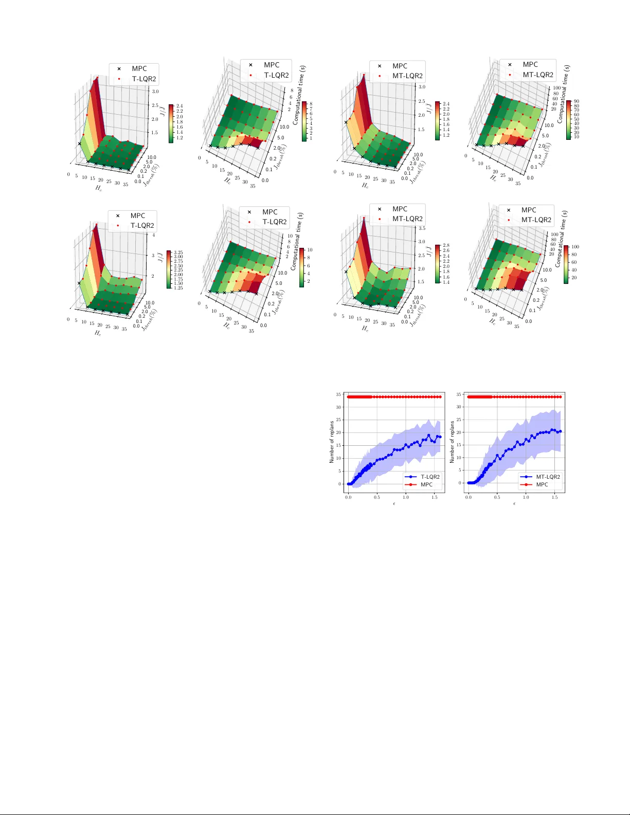
Loading high-quality paper...
Comments & Academic Discussion
Loading comments...
Leave a Comment