Look-Ahead SCOPF (LASCOPF) for Tracking Demand Variation via Auxiliary Proximal Message Passing (APMP) Algorithm

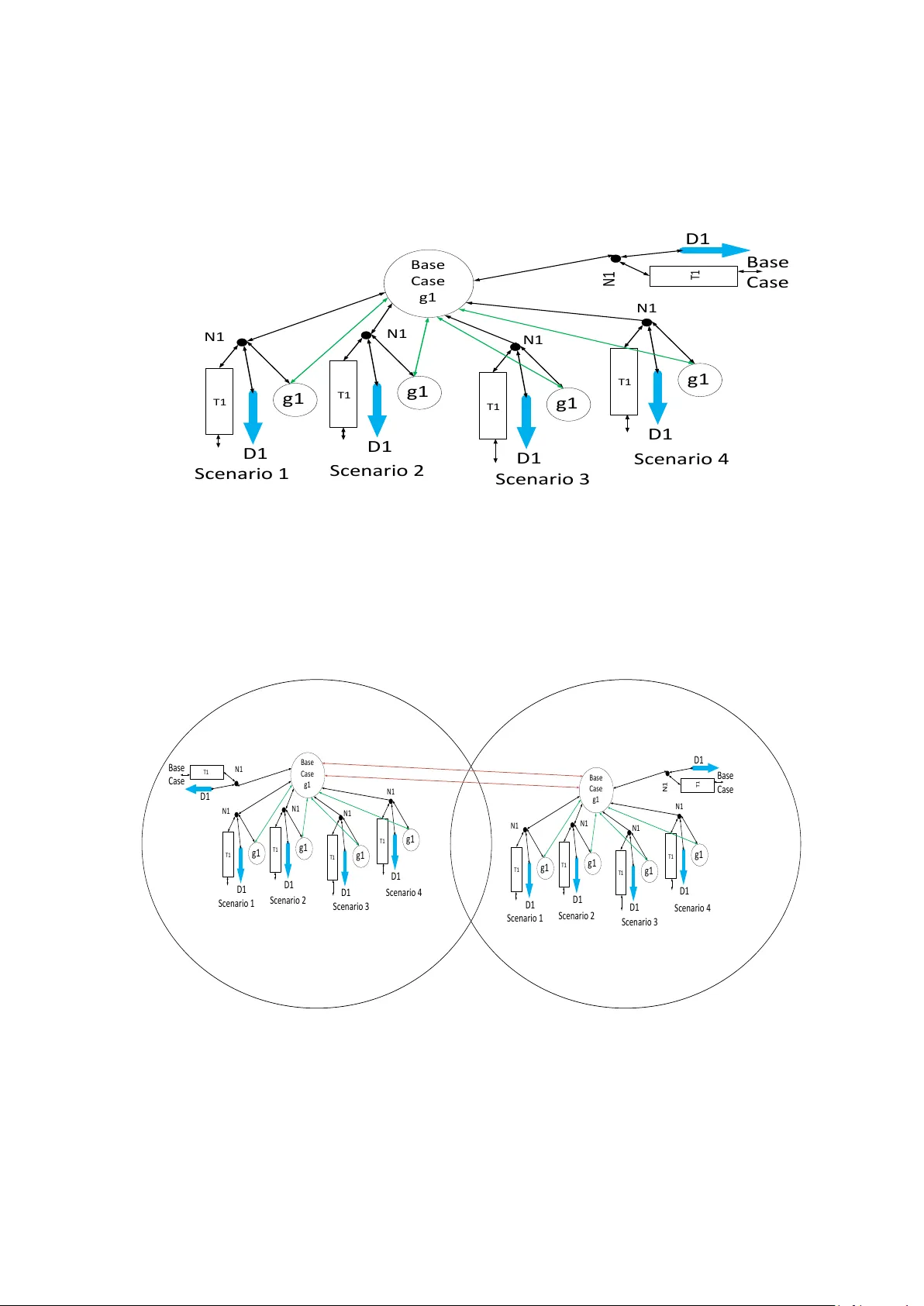
Lo ok-Ahead SCOPF (LASCOPF) for T rac king Demand V ariation via Auxiliary Pro ximal Message P assing (APMP) Algorithm I Sam buddha Chakrabarti a, ∗ , Ross Baldic k a a Dep artment of Ele ctric al & Computer Engine ering (ECE), The University of T exas at Austin, A ustin, TX 78705, USA Abstract In this pap er, w e will consider the Look-Ahead Securit y Constrained Optimal Po w er Flo w (LASCOPF) problem looking forward multiple dispatc h in terv als, in which the load demand v aries ov er dispatc h interv als according to some forecast. W e will consider the base-case and several con tingency scenarios in the up c oming as well as in the subse quent dispatc h in terv als. W e will form ulate and solv e the problem in a Mo del Predictiv e Con trol (MPC) paradigm. W e will present the Auxiliary Pr oximal Message Passing (APMP) algorithm to solve this problem, which is a bi-la yered decomp osition-coordination type distributed algorithm, consisting of an outer A uxiliary Pr oblem Principle (APP) la yer and an inner Pr oximal Message Passing (PMP) la yer. The APP part of the algorithm distributes the computation across several dispatch interv als and the PMP part performs the distributed computation within eac h of the dispatc h interv al across different devices (i.e. generators, transmission lines, loads) and no des or nets. W e will demonstrate the effectiv eness of our metho d with a series of n umerical sim ulations. 1. In tro duction In this pap er, we will consider the ( N − 1) Se curity-Constr aine d Optimal Power Flow (SCOPF) problem, in which devices (i.e. generators, transmission lines, loads etc.) are connected on the p o w er net work and there exists a set of sc enarios — each corresp onding to the failure of a particular transmission line — ov er which we must ensure optimal feasible op eration of the net work. But, instead of solving the SCOPF for the up coming dispatc h interv al only , at the I The ob jective of this pap er is to present nov el algorithmic and computational to ols for solving the Lo ok-Ahead Security Constrained Optimal P ow er Flo w (LASCOPF) accurately , pro v ably , and reasonably fast. It will form a foundation, based on whic h, w e will build up on further impro vemen ts of the algorithm and also the problem. The authors were supp orted, in part, by the National Science F oundation (NSF) under gran t ECCS-1406894. ∗ I am the corresp onding author Email addr esses: schakrabarti@utexas.edu (Sambuddha Chakrabarti), baldick@ece.utexas.edu (Ross Baldick) Pr eprint submitte d to Elsevier Scienc e Dir e ct Power System R ese ar ch Journal Septemb er 19, 2019 start of each such in terv al, w e will also lo ok forward several subsequent dispatch in terv als, in which the load demands change according to a forecast. W e will take into accoun t the ramp rates of generators and op erate the system suc h that the generation cost is minimized, sub ject to the constraints of satisfying the changing load demand, line p o wer flow limit constrain ts, minimum and maxim um generation constraint of each generator, enforced in eac h of the up coming and subsequent dispatc h in terv als considered. The goal is to minimize a comp osite cost function that includes the cost (and constraints) of nominal op eration, as w ell as those asso ciated with constrain ts on op eration in an y of the (adverse) scenarios, for multiple dispatc h in terv als. This results in a large optimization problem, since v ariables in the net work, namely , real p ow er injection and bus voltage phase angle, are rep eated |L| times for eac h of the | Ω | dispatc h in terv als, where |L| is the n umber of con tingencies. Therefore we present a distributed algorithm to solve this problem, whereb y w e break the problem in to sev eral smaller indep enden t sub-problems and solve them in parallel, such that the only co-ordination required is lo cal, through the Lo cational Marginal Prices (LMP) up dates. Sp ecifically , we use a suitably mo dified version of the message passing algorithm from [1] and [2] to solv e this problem efficien tly . F or simplicity , w e consider only DC p o wer flo w in this pap er. The extension to AC p o w er flo w, inv olv es simply applying the A C-OPF mo del from [ 3 ], [ 4 ], [ 5 ], [ 6 ], [ 7 ], and [ 8 ] to each scenario and requiring that the phase angles of a given device are equal across all scenarios in the resp ectiv e time p eriods. In the previous works in [ 1 ], [ 9 ], and [ 2 ], Kraning et al. , applied the Proximal Message P assing Algorithm to solve the standard Static Optimal Po w er Flo w (OPF) Problem while Liu et al. and Chakrabarti et al. resp ectiv ely applied it to solve the ( N − 1) Securit y Constrained OPF (SCOPF). In this pap er, w e extend this approac h to solving a lo ok-ahead dispatc h problem, which considers the v ariation of load o ver a time horizon. There can b e interesting and direct underpinnings of solving suc h problems when it comes to design and allo cation of Financial T ransmission Rights (FTRs) under random outages, as well [ 10 ]. Our formulation for the LASCOPF is based on the Mo del Predictiv e Control (MPC) or Receding Horizon Control (RHC) metho dology [ 11 , 12 , 13 , 14 , 15 ]. The rest of the pap er is organized as follows: In section 2 we present a brief literature survey , after which, in section 3 we introduce the system of notations and present the con ven tional form ulation of lo ok-ahead SCOPF in the “Angles Represented” version, where the differen t real p o w er flo ws on the T ransmission Lines are represented in terms of the real p o w ers injected at the buses and the v oltage phase angles at the buses. In section 4, w e apply the coarse-grained APP decomp osition to split the problem in to different dispatch interv als. In section 5, we reform ulate all the preceding SCOPF problems (b elonging to differen t dispatch in terv als) in to a different framework, the D T N (Devices-T erminals-Nets) formulation, which is particularly suitable for applying the ADMM (Alternating Direction Metho d of Multipliers) [ 16 ] based Pro ximal Message P assing algorithm to the problems. In section 6, w e present the Proximal Message Passing fine-grained decomp osition for the present problem. In section 7, w e present the results of some sim ulation studies conducted on the IEEE test systems and we dra w the concluding remarks and p oin t to future researc h in section 8. 2 2. Literature Surv ey and Related w ork The Optimal P ow er Flo w Problem is at the heart of Po w er Systems planning and op erations. Initially form ulated b y Carp en tier in [ 17 ], it has been studied for more than half a cen tury , and has extensively b een applied in the industry as w ell, including solving the electricity market sc heduling and dispatch calculations b y the ISOs/TSOs (which inv olv es solving the DC-OPF) and applications by the market participants for planning using pro duction-cost mo deling systems, like Uplan [ 18 ]. Happ in [ 19 ] and Cho wdhury & Rahman in [ 20 ] trace the historical dev elopment of OPF upto the 90s. A recent reference that provides a go o d summary of the historical developmen t of the problem is Cain, O’Neill and Castillo [ 21 ]. The references cited there also pro vide go od insights into form ulation and mo deling particularly , of the A COPF. There has b een recen tly a surge in the interest in ACOPF following the works of Bai et al. in [ 3 ] and La v aei et al. in [ 4 ], [ 5 ], [ 6 ], [ 7 ], where the authors sho wed that the A COPF problem can b e solved accurately by a con vex relaxation of the original problem into a Semidefinite Programming problem. In reference [ 22 ], the authors hav e presented the AC-OPF conv ex relaxations using Second Order Cone Programming (SOCP) for branch flo w mo dels, while reference [ 23 ] by Lo w pro vides an excellent and comprehensiv e guide to the curren t state of researc h in A C-OPF conv ex relaxation, making a sp ecial mention of the theory of c hordal graphs, clique tree-decomp osition, and SDP , as applied to p o wer net works. Utlilizing these t wo ideas, recen t references [ 24 ] and [ 25 ] men tion applying distributed algorithms to AC-OPF, resp ectiv ely , in the con texts of a distribution lev el microgrid and reactive p o wer compensation. Reference [ 26 ] illustrates application of ADMM to sparse SDP for solving A C-OPF. In the recen t reference [ 27 ], the authors presented a mo dified version of the ADMM, showing that a global optim um for the highly non-conv ex AC-OPF can b e obtained by applying this algorithm. The recent trend of applying distributed optimization algorithms to p o wer flow problems in order to sp eed up the computation time has gained ample momentum already . Tw o of the recent pap ers that pro vide v ery go od and comprehensive comparisons b et w een the p erformance of sev eral different algorithms for solving the OPF and SCOPF problems are [ 28 ] and [ 29 ], where the authors men tioned ADMM, Proximal Message passing (PMP), APP , Consensus+Inno v ation (C+I), Optimalit y Condition Decomp osition (OCD) etc. algorithms. The pioneering w ork on the Security Constrained OPF (SCOPF) was done by Stott et al in [ 30 ]. Some of the recent references include works by Chiang et al. [ 31 ], Phan et al. [ 32 ], Chakrabarti et al. [ 2 ] etc. The last tw o deal with application of distributed algorithms to the SCOPF problem. In [ 8 ] and in [ 9 ], the authors hav e applied ADMM to solve the A COPF and SCOPF, but not to a lo ok-ahead problem. Significan t early works on ADMM metho d during the 70s and 80s were [ 33 ], [ 34 ], [ 35 ] etc. follo wed by w ork during the 90’s which include [ 36 ], [ 37 ]. Combining these tw o fields gives rise to the Distributed Computational metho ds for OPF [ 38 ], [ 39 ]. The last reference provides a go o d comparison of the distributed metho ds till the end of 90s. Go od references on Mo del Predictive Control (MPC) or Receding Horizon Con trol (RHC) are [11, 12, 13, 14, 15]. 3 2.1. Con tribution of the Presen t W ork While there has b een some excellen t w ork in the recent past on ( N − 1) and ( N − k ) SCOPFs as evidenced b y references [ 40 , 41 , 42 , 43 , 44 ], there is a dearth of literature on m ultiple-dispatch interv al SCOPF. Also, a v ast ma jorit y of the academic literature presen t till date on the topic of SCOPF either solve a correctiv e con trol version of the SCOPF (by c hanging generator dispatch to relieve line congestion in the outaged cases) or they solve a chance constrained version. Moreov er, in the academic b ody of literature, there is also a sev ere lack of materials describing the soft ware implementation for SCOPF and LASCOPF for the prev entiv e con trol version. The main contribution of our w ork, in the light of the ab o v e, can b e summarized as presen ting the preven tiv e control version of ( N − 1) SCOPF for multiple dispatch interv als, as a part of whic h, we hav e also dev elop ed a softw are for implemen ting the mathematical mo del and the algorithms, which utilizes a t wo-la y ered distributed algorithm. In our present work, we will b e solving the Lo ok-Ahead Security Constrained Optimal Po w er Flow (LASCOPF) problem, formulated in a MPC/RHC format, using a combination of APP and ADMM-PMP algorithms, which w e will call the APMP algorithm. As in all MPC/RHC form ulations, the implicit assumption will b e that this problem for several lo ok-ahead dispatc h in terv als is solv ed at the b eginning of each dispatc h in terv al, up dating the forecasts, thereby reac hing the b est accuracy and abilit y to track the time-v arying load demand. 2.2. Comparison of the Presen t Algorithm Against Other Metho ds In the present metho d, that we are ab out to describ e in this pap er, the heart of the problem lies in solving the OPF problem using ADMM-PMP , while using APP to reach consensus among m ultiple different OPFs that we solve. There are other metho ds also to achiev e the same goal. It’s hard to say , which metho d is sup erior to which one. There are man y factors and considerations, and the merit of a particular metho d dep ends on what factors are considered important, for a particular application. In the ligh t of that, in the recen t pap ers, [ 29 ] and [ 28 ] w e ha ve made comparisons against sev eral differen t metho ds, which can b e summarized as b elo w: The differen t algorithms compared are Analytical T arget Cascading (A TC), ADMM (the pristine version), ADMM-PMP , APP , Optimalit y Condition Decomp osition (OCD), and Consensus+Inno v ation (C+I) in the light of the follo wing factors: • Pr esenc e of a c entr al c o or dinator: While A TC and ADMM do need cen tral co ordinators, ADMM-PMP , APP , OCD, and C+I do not need a central co ordinator. This can sp eed up computations b y reducing b ottlenec k of communication time with co ordinator. • Computations Effort: F or a single iteration, ADMM-PMP and C+I has got m uch less computational effort as compared to all the other algorithms. How ev er, ADMM-PMP needs many more iterations to conv erge. In our case, w e compromised on accuracy , in order to cut down on the ADMM-PMP iterations. In order to solve the LASCOPF, 4 since we need to wrap the ADMM-PMP lay er with the APP outer lay ers, we cannot help reduce the net computational burden. Ho wev er, it is considerably less than had an y of the other metho ds b een used. • Data Exchange d and Shar e d: ADMM-PMP has a high v olume of data exchanged and shared as compared to the other algorithms. Ho wev er, giv en the previous p oint, com bined with the fact that the data shared and exchanged volume of APP is quite lo w, the net comm unication time of APMP is mo derate. F rom the ab o ve comparison, we can conclude that APMP is a go o d candidate for distributed algorithm for solving LASCOPF problems. Certainly , for big netw orks and many con tingency scenarios and dispatch in terv als, we wouldn’t prefer a centralized algorithm. Given b elo w, is a table (T able 1) indicating comparison of APMP against a cen tralized solv er implemen ted with GUROBI, as a b enc hmark solv er. The p ercen tage difference in optimal ob jectiv e v alue is calculated as: % Difference = (APMP Optimal Ob jectiv e − Centralized Optimal Ob jectiv e) × 100 Centralized Optimal Ob jective T able 1: Comparison of APMP against Cen tralized b enc hmark. T yp e of the System P ercentage Difference 5 bus 0 14 bus 0.101128791 30 bus 0 57 bus -0.003811375 118 bus 0 300 bus -0.0001387213 3. Con v en tional Lo ok-Ahead SCOPF F orm ulation In this section, we will formulate the mo dels for the lo ok-ahead SCOPF in the con ven tional framew ork. First w e will introduce the notations and symbols to b e used for the rest of the pap er, whic h are same as those in tro duced in [2] with a few additions. 3.1. Notations and Con v en tions W e ha ve categorized the en tities used in the subsequen t formulations in to fiv e differen t groups: Sets, Elements, Index, Parameters, and V ariables. • Sets D : Set of Devices The next three sets form partitions of the set of devices: 5 G ⊆ D : Set of Generators T ⊆ D : Set of T ransmission Lines L ⊆ D : Set of Loads T : Set of T erminals N : Set of Nets or Buses or No des J ( N i ): Set of buses/no des/nets directly connected to no de N i ∈ N L = { 0 , 1 , 2 , ..., |L|} : Set of p ossible ( N − 1) Contingencies. The element 0 indicates the base case Ω = { 0 , 1 , 2 , ..., | Ω |} : Set of Dispatc h interv als or, the net Dispatch Horizon under consideration. 1 indicates the up coming dispatch in terv al under consideration, for whic h a dispatch decision will definitely b e implemented. The rest, { 2 , 3 , ..., | Ω |} , are subsequen t in terv als in future. Hence, dispatc h in terv al 0 is the curren t running one. † will b e used to denote the transp ose of a vector or matrix. • Elements t : Elemen ts of T g : Elements of G D : Elements of L T : Elements of T N : Elements of N • Indic es i, j : Nets k : T erminals q : Generators r : T ransmission Lines d : Loads c : Con tingencies τ : Dispatch In terv als ν : Iteration coun t for ADMM/PMP algorithm µ AP P : Iteration count for APP algorithm • Par ameters R T r , X T r , Z T r = R T r + ( √ − 1 ) X T r , B T r : Resistance, Reactance, Imp edance, and Susceptance of the r th T ransmission Line, resp ectiv ely 6 α , β , γ : APP tuning parameters, ρ : ADMM-PMP tuning parameter α g q , β g q , γ g q : Quadratic, Linear, and Constan t Cost Co-efficients of the q th Gener- ator C g q ( . ) , f dev ( . ) will b e used to denote the cost function of the g q th generator and that of a generic device, resp ectiv ely , throughout. W e will introduce the other cost functions in the appropriate sections I ≤ ( . ), I ≥ ( . ), I = ( . ): Indicator functions such that I ≤ ( x ) = 0, if 0 ≤ x , and = ∞ otherwise, and similarly for I ≥ ( . ) and I = ( . ) P g q , P g q , R g q , R g q (= − R g q ,usually), L T r denote the maxim um and minim um gener- ating limits of generators, maxim um ramp-up and ramp-do wn limits of generators, and p o wer carrying capacity of transmission lines resp ectiv ely • V ariables P : The real p ow er or, MW asso ciated with different devices θ : The bus v oltage phase angles asso ciated with different no des, as well as the devices λ : The lagrange multiplier or dual v ariable corresp onding to the consensus among differen t p o w er generation v ariables b et ween the dispatc h in terv als The follo wing is the conv en tion w e follow in order to iden tify the asso ciations of an y particular v ariable to the sets:  x ( p 3 )( p 4 ) d ( p 1 )( p 2 )  ( ν ) . In the ab o ve, x d is a v ariable asso ciated with a device-terminal or no de/net-terminal, d . ( p 1 )( p 2 ) and ( p 3 )( p 4 ) indicate the computational units/agen ts, denoted, resp ectiv ely , b y a com bination of p 1 , p 2 and p 3 , p 4 , where a particular p i ma y refer to either a dispatc h interv al or contingency scenario it is asso ciated with. The combination ( p 1 )( p 2 ) denotes a particular computational agen t linked to this particular combination. The ab o v e notation should b e in terpreted as the b elief ab out the v alue of the v ariable, x d asso ciated or linked to the sup erscripted computational agen t ( ( p 3 )( p 4 ) ), as held by the subscripted computational agent ( ( p 1 )( p 2 ) ) at the ν − th iteration. Let’s tak e a lo ok at the next example, to mak e the meaning clearer.  P ( c 2 )( τ 2 ) N t ( c 1 )( τ 1 )  ( ν ) . The foregoing notation refers to the b elief of the v alue of a v ariable P N t asso ciated with a particular terminal, N t , (whic h is indexed b y the t ) of either a net or a device for the con tingency scenario indexed by c 2 during τ 2 , as estimated b y a computational agent link ed to τ 1 and contingency scenario, c 1 . Sometimes we will use the net num b er instead of the terminal num b er in the ab ov e con ven tion, when w e w ant to indicate sev eral devices connected to a particular net. If it is part of an iterative algorithm, then the outermost sup erscript ν indicates the iteration count. Whenever a v ariable is b oldface, one or more of the indices will b e missing and that means the b oldface v ariable is a vector each of whose comp onen ts will 7 ha ve all or some of the missing indices (the comp onents themselves can b e v ectors or scalars). When the v ariable is not b old-face and still some of the indices are missing, that means it is a scalar and the missing indices are either irrelev an t or their v alues are implied from the con text. Also it is to b e observed that since generators and loads are single terminal devices, it is not necessary to sp ecify the terminals for these, unless absolutely required. 3.2. Lo ok-Ahead Dispatc h: Generalized Case of Demand V ariation for Multi-Bus Case In this pap er we build on the static SCOPF problem form ulation in [ 2 ]. W e will dev elop the mathematical mo del for a lo ok-ahead dispatc h calculation that considers an up coming and several subsequen t dispatc h interv als at the onset of each current dispatc h interv al and tak es in to accoun t the p ossible v ariations of op erating parameters across different scenarios represen ted in differen t subsequent dispatc h interv als, so that at eac h interv al the en tire system is secure. A t the end of each curren t dispatch interv al, the calculation “rolls forw ard” and the whole lo ok-ahead calculation is rep eated with up dated demand forecast, just as in a “Mo del Predictive Control (MPC)” or a “Receding Horizon Con trol (RHC).” The generalized v ersion of this problem for a multi-time horizon, arbitrary net work is as follows: min P ( τ ) g q ,θ X τ ∈ Ω X g q ∈ G C g q ( P ( τ ) g q ) (1a) Sub ject to : ∀ ( c ) ∈ L , ∀ τ ∈ Ω , ∀ T r ∈ T P ( τ ) g q N i − P ( τ ) D d N i = X N i ∈ J ( N i ) B ( c ) T r ( θ ( c )( τ ) N i − θ ( c )( τ ) N i ); ∀ N i ∈ N (1b) | B ( c ) T r ( θ ( c )( τ ) T r t 1 − θ ( c )( τ ) T r t 2 ) | ≤ L ( c ) T r , ∀ T r ∈ T (1c) R g q ≤ ( P ( τ +1) g q − P ( τ ) g q ) ≤ R g q ∀ g q ∈ G (1d) In the optimization mo del (1), the ob jectiv e function to b e minimized, (1a) represents the total generation cost for all the generators in the system, summed ov er all the lo ok-ahead dispatc h interv als under consideration. The innermost summation is for all the generators and outermost summation is o ver all the future dispatch interv als. There are three sets of constrain ts. The first set of constraints (1b) describ es the no dal p o wer balance. The left-side of the equality represents the no dal p o wer injection, which is the generator output, less the load connected to the particular no de and the right-side of the equality represents the p o w er flo w along all the transmission lines that are connected to the no de (according to the angles represented v ersion of the DC p ow er flo w approximation). Inequality constrain ts (1c) represen t the transmission lines’ pow er flow limits for b oth the base case and each of the con tingency scenarios for all the lines and all the dispatch interv als (the base case as w ell as the scenarios are indexed in the sup erscript with ( c ) and the dispatch interv als, by ( τ )). As b efore, the left-side of the inequality represents the DC (or linearized) approximation of the line p o wer flo w and the righ t-side represen ts the limit. The last set of inequalities (1d) represent the generator ramping constrain ts, where it can b e seen that the change in 8 P ( 1 ) ( 1 ) τ = 1 P ( 2 ) ( 1 ) P ( 2 ) ( 2 ) P ( 1 ) ( 2 ) τ = 2 Figure 1: Sc hematic for APP Message Exchange. τ = 0 P ( 0 ) g 1 P ( 0 ) g 2 P ( 1 ) ( 1 ) τ = 1 P ( 2 ) ( 1 ) P ( 2 ) ( 2 ) P ( 1 ) ( 2 ) τ = 2 P ( 3 ) ( 2 ) P ( 2 ) ( 2 ) P ( 2 ) ( 3 ) τ = 3 P ( 3 ) ( 3 ) P ( 4 ) g 1 P ( 4 ) g 2 τ = 4 Figure 2: Schematic for Lo ok- Ahead SCOPF for Demand V ari- ation generator output from one dispatch in terv al to the other is b ounded b y the maximum and minim um ramping limits of the the generators. 4. APMP Algorithm: The Coarse Grained Decomp osi- tion Comp onen t In this section, we will provide the mathematical formulation of the Auxiliary Pro ximal Message Passing (APMP) algorithm, as applied to the LASCOPF problem. W e will start b y describing the APP based coarse-grained comp onen t of the algorithm, whic h will b e applied to the LASCOPF problems, follow ed b y the PMP fine-grained comp onent, which decomp oses the SCOPF problems (and the OPF problems) of each dispatch interv al into the device level computations. The basic idea b ehind the APP based coarse-grained distributed comp onen t of the algorithm is depicted in figure 1, where the t wo circles corresp ond to differen t dispatch in terv als and/or scenarios, across whic h the computation is split, and the arrows indicate the exc hange of messages b et ween those. The messages corresp ond to the b eliefs of eac h circle or coarse grain ab out the v alues of p o wer generations and/or injections/line flows within itself and also of those b elonging to the neigh b oring circles. 9 4.1. Generalized Case of Demand V ariation for Multi-Bus Case Referring to the figure 2, the differen t ov erlapping circles here represent the different dispatch in terv als, and with τ = 0 and τ = 4 representing resp ectively , the latest dispatc h in terv al for whic h the LASCOPF problem is already solv ed & the results are known, and the dispatch in terv al following the concerned time horizon. In the coarse-grained decomp osition, when τ = 1, P ( τ − 1) g 2 ( τ ) and P ( τ − 1) g 1 ( τ ) are replaced by P (0) g 2 and P (0) g 1 resp ectiv ely , whic h are the (known) MW outputs from the current dispatch interv al. When τ = 3, P ( τ +1) g 2 ( τ ) and P ( τ +1) g 1 ( τ ) are replaced b y P (4) g 2 and P (4) g 1 resp ectiv ely , which are the last but one iterate v alues of the MW outputs from the last dispatc h in terv al. W e will no w apply the Auxiliary Problem Principle (APP)[ 45 ], [ 46 ] to the ab o v e optimization problem to deriv e a set of expressions for the iterate up dates. This reformulation is v ery similar in fla vor to the ones presented previously in [ 38 ], [ 47 ], [ 48 ], [ 49 ] etc. W e will state the coarse-grained APP based decomp osition of the problem (the one for whic h the con v entional form ulation has been presented in equation (1)). W e will distribute the SCOPF across each dispatc h in terv al and then exc hange messages regarding what a particular interv al thinks ab out the optimal v alues of the decision v ariables for the interv als immediately preceding and succeeding it, even tually attempting to achiev e a consensus b et w een those. In the figure, the v alues shown at the t wo sides of the arro ws are those “b eliefs” among which we are trying to achiev e consensus. W e follo w the same con ven tion as introduced in section 3.1. As b efore, notice that each of the subproblems is very similar to the classical ( N − 1) SCOPF problems, but with tw o imp ortan t differences. First of all, eac h of these has ramp rate constrain ts, to accoun t for the c hange in generator outputs ov er m ultiple interv als. Secondly , there are regularization terms added to the cost function for attaining consensus among different coarse grains ab out the v alues of the decision v ariables, whic h, in this case, are generator outputs. The second terms in the ob jectiv e functions are the ones representing the pro ximity from previous iterates. The third and fourth terms in the ob jectiv e functions of equations (2) and (4) and the third, fourth, fifth, and sixth terms in the ob jective function of equation (3) are the ones for attaining consensus among the coarse grains. The last terms in the ob jective functions of equations (2) and (4) and the last t wo terms in the ob jectiv e function of equation (3) corresp ond to complementary slac kness. Note that, in this case also, the real p o wer generation v ariables are the only ones at which w e wish to attain consensus through the application of APP . The bus v oltage angles can b e though t of as lo calized to the particular dispatc h int erv al sub-problems, whose v alues at an y iteration are determined b y the p o w er generation or injection profiles. W e ha ve split the LASCOPF problem in to three t yp es of sub-problems, each corresp onding to a particular dispatc h time interv al. First Dispatch Interv al SCOPF: P ( 1 ) ( µ AP P +1) = argmin P ( 1 ) ,θ X g q ∈ G C g q ( P (1) g q (1) )+ β 2 || P ( 1 ) − P ( 1 ) ( µ AP P ) || 2 2 10 + γ [ P ( 1 ) ( 1 ) † ( P ( 1 ) ( 1 ) ( µ AP P ) − P ( 1 ) ( 2 ) ( µ AP P ) )+ P ( 2 ) ( 1 ) † ( P ( 2 ) ( 1 ) ( µ AP P ) − P ( 2 ) ( 2 ) ( µ AP P ) )] + λ 1 ( µ AP P ) † P ( 1 ) ( 1 ) + λ 2 ( µ AP P ) † P ( 2 ) ( 1 ) (2a) Sub ject to : ∀ ( c ) ∈ L , ∀ T r ∈ T P ow er-Balance Constrain ts (Base-Case & Contingency): P (1) g q N i (1) − P (1) D d N i = X N i ∈ J ( N i ) B ( c ) T r ( θ ( c )(1) N i − θ ( c )(1) N i ); ∀ N i ∈ N (2b) Flo w Limit Constraints (Base-Case & Contingency): | B ( c ) T r ( θ ( c )(1) T r t 1 − θ ( c )(1) T r t 2 ) | ≤ L ( c ) T r , ∀ T r ∈ T (2c) Ramp-Rate Constraints: R g q ≤ P (2) g q (1) − P (1) g q (1) ≤ R g q , ∀ g q ∈ G (2d) R g q ≤ P (1) g q (1) − P (0) g q ≤ R g q , ∀ g q ∈ G (2e) In the coarse-grained decomp osed sub-problem (2), which is for the first lo ok-ahead dispatch in terv al, the only differences from optimization mo del (1) are that, in the ob jective function, (2a) we don’t hav e the summation o ver the dispatc h interv als, for obvious reason, since the computation is split across the dispatc h interv als. Also, w e can see that, the ob jectiv e function has some additional regularization terms. And as mentioned in the last paragraph, these are regularization terms added to the cost function for attaining consensus among differen t coarse grains ab out the v alues of the decision v ariables, whic h, in this case, are generator outputs. The second terms in the ob jectiv e function is the one representing the pro ximity from previous iterate, P ( 1 ) ( µ AP P ) . The third and fourth terms in the ob jectiv e function (2a) are the ones for attaining consensus among the coarse grains. That is, in the third term, attaining consensus b et w een P ( 1 ) ( 1 ) ( µ AP P ) , whic h are the b eliefs of in terv al 1 ab out its o wn generator outputs and P ( 1 ) ( 2 ) ( µ AP P ) , which are the b eliefs of interv al 2 ab out the generator outputs of in terv al 1. The fourth term has a similar in terpretation as to attaining consensus among interv al 1’s b eliefs of generator outputs of interv al 2 and interv al 2’s b eliefs ab out its o wn. The last tw o terms in the ob jectiv e function corresp ond to complementary slac kness. Note that, in this case also, the real p o w er generation v ariables are the only ones at which we wish to attain consensus through the application of APP . The bus voltage angles can b e though t of as lo calized to the particular dispatch in terv al sub-problems, whose v alues at any iteration are determined b y the p o w er generation or injection profiles. The rest of the constraints corresp onding to the no dal p ow er balance, line flow limits, and generator ramping are exactly the same as those app earing in (1). In termediate Dispatch In terv al τ ∈ { 2 , 3 , ..., | Ω | − 1 } SCOPF: P ( τ ) ( µ AP P +1) = argmin P ( τ ) ,θ X g q ∈ G C g q ( P ( τ ) g q ( τ ) )+ 11 β 2 || P ( τ ) − P ( τ ) ( µ AP P ) || 2 2 + γ [ P ( τ − 1 ) ( τ ) † ( P ( τ − 1 ) ( τ ) ( µ AP P ) − P ( τ − 1 ) ( τ − 1 ) ( µ AP P ) )+ P ( τ ) ( τ ) † ( P ( τ ) ( τ ) ( µ AP P ) − P ( τ ) ( τ − 1 ) ( µ AP P ) ) + P ( τ ) ( τ ) † ( P ( τ ) ( τ ) ( µ AP P ) − P ( τ ) ( τ + 1 ) ( µ AP P ) )+ P ( τ + 1 ) ( τ ) † ( P ( τ + 1 ) ( τ ) ( µ AP P ) − P ( τ + 1 ) ( τ + 1 ) ( µ AP P ) )] + λ 2 τ − 1 ( µ AP P ) † P ( τ ) ( τ ) + λ 2 τ ( µ AP P ) † P ( τ + 1 ) ( τ ) − λ 2 τ − 3 ( µ AP P ) † P ( τ − 1 ) ( τ ) − λ 2 τ − 2 ( µ AP P ) † P ( τ ) ( τ ) (3a) Sub ject to : ∀ ( c ) ∈ L , ∀ T r ∈ T P ow er-Balance Constrain ts (Base-Case & Contingency): P ( τ ) g q N i ( τ ) − P ( τ ) D d N i = X N i ∈ J ( N i ) B ( c ) T r ( θ ( c )( τ ) N i − θ ( c )( τ ) N i ); ∀ N i ∈ N (3b) Flo w Limit Constraints (Base-Case & Contingency): | B ( c ) T r ( θ ( c )( τ ) T r t 1 − θ ( c )( τ ) T r t 2 ) | ≤ L ( c ) T r , ∀ T r ∈ T (3c) Ramp-Rate Constraints: R g q ≤ P ( τ +1) g q ( τ ) − P ( τ ) g q ( τ ) ≤ R g q , ∀ g q ∈ G (3d) R g q ≤ P ( τ ) g q ( τ ) − P ( τ − 1) g q ( τ ) ≤ R g q , ∀ g q ∈ G (3e) In the coarse-grained decomp osed sub-problem (3), which are for the intermediate dispatch in terv als, as opp osed to the ob jectiv e function for the optimization problem for the first dispatc h interv al, in (3a) there are four regularization terms after the one represen ting the pro ximity from previous iterate, P ( τ ) ( µ AP P ) . The third term is for attaining consensus b et w een P ( τ − 1 ) ( τ ) ( µ AP P ) , which are the b eliefs of in terv al τ ab out the generator outputs of interv al τ − 1 and P ( τ − 1 ) ( τ − 1 ) ( µ AP P ) , which are the b eliefs of interv al τ − 1 ab out its own generator outputs. The fourth term has a similar interpretation as to attaining consensus among in terv al τ ’s b eliefs of its o wn generator outputs and interv al ( τ − 1)’s b eliefs ab out generator outputs of interv al τ , whereas the fifth term p ertains to attaining consensus among interv al τ ’s b eliefs of its own generator outputs and in terv al ( τ + 1)’s b eliefs ab out generator outputs of interv al τ . The sixth term p ertains to attaining consensus among the b elief of interv al τ ab out generator outputs of interv al τ + 1 and b elief of interv al τ + 1 ab out its own generator outputs. The last four terms in the ob jectiv e function corresp ond to complementary slackness. The rest of the constraints corresp onding to the no dal p ow er balance, line flow limits, and generator ramping are again, exactly the same as those app earing in (1). Last Dispatch Interv al, or Dispatc h Interv al | Ω | SCOPF: P ( | Ω | ) ( µ AP P +1) = argmin P ( | Ω | ) ,θ X g q ∈ G C g q ( P ( | Ω | ) g q ( | Ω | ) )+ 12 β 2 || P ( | Ω | ) − P ( | Ω | ) ( µ AP P ) || 2 2 + γ [ P ( | Ω |− 1 ) ( | Ω | ) † ( P ( | Ω |− 1 ) ( | Ω | ) ( µ AP P ) − P ( | Ω |− 1 ) ( | Ω |− 1 ) ( µ AP P ) )+ P ( | Ω | ) ( | Ω | ) † ( P ( | Ω | ) ( | Ω | ) ( µ AP P ) − P ( | Ω | ) ( | Ω |− 1 ) ( µ AP P ) )] − λ 2 | Ω |− 3 ( µ AP P ) † P ( | Ω |− 1 ) ( | Ω | ) − λ 2 | Ω |− 2 ( µ AP P ) † P ( | Ω | ) ( | Ω | ) (4a) Sub ject to : ∀ ( c ) ∈ L , ∀ T r ∈ T P ow er-Balance Constrain ts (Base-Case & Contingency): P ( | Ω | ) g q N i ( | Ω | ) − P ( | Ω | ) D d N i = X N i ∈ J ( N i ) B ( c ) T r ( θ ( c )( | Ω | ) N i − θ ( c )( | Ω | ) N i ); ∀ N i ∈ N (4b) Flo w Limit Constraints (Base-Case & Contingency): | B ( c ) T r ( θ ( c )( | Ω | ) T r t 1 − θ ( c )( | Ω | ) T r t 2 ) | ≤ L ( c ) T r , ∀ T r ∈ T (4c) Ramp-Rate Constraints: R g q ≤ P ( | Ω | )( µ AP P ) g q ( | Ω | ) − P ( | Ω | ) g q ( | Ω | ) ≤ R g q , ∀ g q ∈ G (4d) R g q ≤ P ( | Ω | ) g q ( | Ω | ) − P ( | Ω |− 1) g q ( | Ω | ) ≤ R g q , ∀ g q ∈ G (4e) Dual V ariable Up dates : λ τ ( µ AP P +1) = λ τ ( µ AP P ) + α ( P ( τ ) ( τ ) ( µ AP P +1) − P ( τ ) ( τ + 1 ) ( µ AP P +1) ) (4f ) λ τ + 1 ( µ AP P +1) = λ τ + 1 ( µ AP P ) + α ( P ( τ + 1 ) ( τ ) ( µ AP P +1) − P ( τ + 1 ) ( τ + 1 ) ( µ AP P +1) ) (4g) Lastly , in the coarse-grained decomp osed sub-problem (4), which is for the last dispatch in terv al under consideration, in the ob jectiv e function for the optimization problem (4a) the tw o regularization terms after the one representing the proximit y from previous iterate, P ( | Ω | ) ( µ AP P ) . The third term is for attaining consensus b et ween P ( | Ω |− 1 ) ( | Ω | ) ( µ AP P ) , whic h are the b eliefs of in terv al | Ω | ab out the generator outputs of interv al | Ω | − 1 and P ( | Ω |− 1 ) ( | Ω |− 1 ) ( µ AP P ) , whic h are the b eliefs of interv al | Ω | − 1 ab out its own generator outputs. The fourth term has a similar interpretation as to attaining consensus among interv al | Ω | ’s b eliefs of its o wn generator outputs and in terv al ( | Ω | − 1)’s b eliefs ab out generator outputs of in terv al | Ω | . The last tw o terms in the ob jective function corresp ond to complementary slac kness. The rest of the constraints corresp onding to the no dal p ow er balance, line flow limits, and generator ramping are again, exactly the same as those app earing in (1). Equations (4f) and (4g) p ertain to up dates of the dual v ariables or the Lagrange multipliers, λ s corresp onding to the differen t p o w er generation consensus terms describ ed ab o v e. The lack of consensus gives the step direction, while α is the step length, as can b e seen ab o ve. W e ha ve presented a coarse grained parallelization of the lo ok-ahead SCOPF to cop e with demand v ariation, where the entire problem is decomp osed across the differen t dispatch time in terv als. Subsequently , we will presen t the ADMM-Proximal Message Passing based fine 13 grained decomp osition and parallelization of the problem. 5. D T N Reform ulations of the SCOPF Problems In this section w e carry out the reformulation of the SCOPF mo dels that we present ed in the last section within eac h APP coarse grain, in order for us to b e able to solv e those problems b y the Proximal Message Passing metho d. In order to simplify the presentation and also b etter clarify the meaning of each term, we will group the terms of the ob jectiv e into four differen t categories. W e will define them and write down the expressions p ertaining to the SCOPF in the coarse grain corresp onding to equation (3). These are: 1) Cost of Generation ( C ( P )): This term consists of the actual total cost of generating real p ow er b y the differen t generators as w ell as the indicator functions corresp onding to the lo wer and upp er generating limits of the differen t generators. F or this term, the real p o wer generated is alw ays considered at the base case. This term is given as: C ( P ( 0 )( τ ) ) = P | G | t k ∈ g q ∩T ,q =1  C g q ( P (0)( τ ) g q t k ( τ ) ) + I ≤ ( P g q − P (0)( τ ) g q t k ( τ ) ) + I ≤ ( P (0)( τ ) g q t k ( τ ) − P g q ) + β 2  ( P (0)( τ ) g q t k ( τ ) − P (0)( τ )( µ AP P ) g q t k ( τ ) ) 2 + P s = − 1 , 1 ( P (0)( τ + s ) g q t k ( τ ) − P (0)( τ + s )( µ AP P ) g q t k ( τ ) ) 2  + γ  P s = − 1 , 1 ( P (0)( τ ) g q t k ( τ ) ( P (0)( τ )( µ AP P ) g q t k ( τ ) − P (0)( τ )( µ AP P ) g q t k (0)( τ + s ) ) + P (0)( τ + s ) g q t k ( τ ) ( P (0)( τ + s )( µ AP P ) g q t k ( τ ) − P (0)( τ + s )( µ AP P ) g q t k (0)( τ + s ) ))  + ( λ ( µ AP P ) g q 2( τ − 1) − λ ( µ AP P ) g q (2 τ − 2) ) P (0)( τ ) g q t k ( τ ) + λ ( µ AP P ) g q (2 τ ) P (0)( τ +1) g q t k ( τ ) − λ ( µ AP P ) g q (2 τ − 3) P (0)( τ − 1) g q t k ( τ )  F or the sake of brevity , we are presenting here the terms corresp onding to line flo w limit con- strain t ( F ( P ( c )( τ ) )), p ow er-angle relation ( χ ( P ( c )( τ ) , θ ( c )( τ ) )), and ramp constraint (∆( P (0)( τ ) )) in the most general and condensed forms. The details of these can b e found in [ 2 ] and [ 50 ]. 2) Line Flo w Limit Constrain t ( F ( P )): This term consists of the sum of the indicator functions corresp onding to enforcing that real p o wer flows on the lines are less than the maxim um allo wed, b oth at the base-case as w ell as under different con tingencies. This term can b e written as: F ( P ( c )( τ ) ) = P ( c ) ∈L P T r ∈ T P t k ∈ T r ∩T I ≤ ( L ( c ) T r − | P ( c )( τ ) T r t k | ) 3) P o w er-Angle Relation ( χ ( P , θ )):This term consists of the sum of the indicator functions corresp onding to the relation of the p o w er flo w at each end of the lines and the voltage phase angles at the t wo ends, b oth at the base-case and the con tingencies. This term can b e written as: χ ( P ( c )( τ ) , θ ( c )( τ ) ) = P ( c ) ∈L P T r ∈ T P t k ,t k 0 ∈ T r ∩T I = P ( c )( τ ) T r t k + θ ( c )( τ ) T r t k − θ ( c )( τ ) T r t k 0 X ( c ) T r ! 4) Ramp Constrain t (∆( P )):This term corresp onds to the change of p o wer output of generator from one time p eriod to another and the maximum rate at which it can go up or do wn. This term can b e written as: ∆( P (0)( τ ) ) = P s = − 1 , 1 P | G | t k ∈ g q ∩T ,q =1 ( I ≤ ( R g q − P (0)( τ + s ) g q t k ( τ ) + P (0)( τ ) g q t k ( τ ) ) + I ≤ ( P (0)( τ + s ) g q t k ( τ ) − P (0)( τ ) g q t k ( τ ) − R g q )) 14 The reformulated equations for the problem stated in equations (2)-(4) are as follo ws: min P ( c )( τ ) t k ,θ ( c )( τ ) t k f ( P ) = C ( P (0)( τ ) ) + F ( P ( c )( τ ) )+ χ ( P ( c )( τ ) , θ ( c )( τ ) ) + ∆( P (0)( τ ) ) (5a) Sub ject to: ˆ P ( c )( τ ) N i t k = 0 , ˜ θ ( c )( τ ) N i t k = 0 , ∀ N i ∈ N , ∀ t k ∈ T , ∀ ( c ) ∈ L (5b) In the ab o ve set of equations, ˆ P ( c )( τ ) N i t k is the av erage no de p o w er injection and ˜ θ ( c )( τ ) N i t k is the deviation of the voltage phase angle of each device connected to a particular no de from the a verage no de v oltage phase angle. Readers are referred to [ 2 ], [ 1 ] for more information on these. Hence, constraints stated in equation (5b) represen t the Kirc hhoff ’s la w for no de p o w er balance and angle consistency . 6. APMP Algorithm: The Fine Grained Decomp osition Comp onen t In this section we state the equations for the Pro ximal Message Passing algorithm based fine-grained decomp osition of the ab o ve problem. 6.1. Pro ximal Message P assing for the Lo ok-Ahead Dispatc h: Gen- eralized Case of Demand V ariation for the Multi Bus-Case F rom equation (5), the sligh tly reform ulated D T N equations are as follows: min P ( c ) t k ,θ ( c ) t k C ( P (0)( τ ) ) + F ( P ( c )( τ ) ) + χ ( P ( c )( τ ) , θ ( c )( τ ) )+ ∆( P (0)( τ ) ) + P ( c ) ∈L P N i ∈N ( ˆ I ( z ( c )( τ ) N i t k ) + ˜ I ( ξ ( c )( τ ) N i t k )) Sub ject to: P ( c )( τ ) t k = z ( c )( τ ) t k , θ ( c )( τ ) t k = ξ ( c )( τ ) t k , ∀ N i ∈ N , ∀ t k ∈ T , ∀ ( c ) ∈ L (6) where ˆ I ( z N i t k ) and ˜ I ( ξ N i t k ) are indicator functions of the sets { z t k | ˆ z N i t k = 0 } and { ξ t k | ˜ ξ N i t k = 0 } resp ectiv ely . Again, for the sake of brevity , we will skip writing do wn the iterates for the transmission lines and loads (which are simple pro jections), and make a mention that they are the same as the ones presen ted in references [2] and [50]. 6.1.1. Iterates for Generators The iterates for generators consist of the up date equations for the real p o w er output and v oltage-phase angles of the generator terminals for b oth the base case and the differen t 15 ( N − 1) contingency scenarios and are as follows: ( P (0)( τ )( ν +1) g q t k , θ ( c )( τ )( ν +1) g q t k ) = argmin P (0)( τ ) g q t k ,θ ( c )( τ ) g q t k [ C g q ( P (0)( τ ) g q t k ( τ ) ) + I ≤ ( P g q − P (0)( τ ) g q t k ( τ ) ) + I ≤ ( P (0)( τ ) g q t k ( τ ) − P g q ) + β 2 [( P (0)( τ ) g q t k ( τ ) − P (0)( τ )( µ AP P ) g q t k ( τ ) ) 2 + P s = − 1 , 1 ( P (0)( τ + s ) g q t k ( τ ) − P (0)( τ + s )( µ AP P ) g q t k ( τ ) ) 2 ]+ γ [ P s = − 1 , 1 ( P (0)( τ ) g q t k ( τ ) ( P (0)( τ )( µ AP P ) g q t k ( τ ) − P (0)( τ )( µ AP P ) g q t k (0)( τ + s ) ) + P (0)( τ + s ) g q t k ( τ ) ( P (0)( τ + s )( µ AP P ) g q t k ( τ ) − P (0)( τ + s )( µ AP P ) g q t k (0)( τ + s ) ))]+ ( λ ( µ AP P ) g q 2( τ − 1) − λ ( µ AP P ) g q (2 τ − 2) ) P (0)( τ ) g q t k ( τ ) + λ ( µ AP P ) g q (2 τ ) P (0)( τ +1) g q t k ( τ ) − λ ( µ AP P ) g q (2 τ − 3) P (0)( τ − 1) g q t k ( τ ) + ∆( P (0)( τ ) )+ P ( c ) ∈L ( ρ 2 )( || P (0)( τ ) g q t k − z ( c )( τ )( ν ) g q t k + u ( c )( τ )( ν ) g q t k || 2 2 + || θ ( c )( τ ) g q t k − ξ ( c )( τ )( ν ) g q t k + v ( c )( τ )( ν ) g q t k || 2 2 )] , ∀ g q ∈ G, τ ∈ Ω , t k ∈ T ∩ G 6.1.2. Iterates for Nets W e are writing here just the analytical forms already derived in [1]. ∀ N i ∈ N , ∀ t k ∈ T ∩ N i , ∀ ( c ) ∈ L , τ ∈ Ω z ( c )( τ )( ν +1) N i t k = u ( c )( τ )( ν ) N i t k + P ( c )( τ )( ν +1) N i t k − ˆ u ( c )( τ )( ν ) N i t k − ˆ P ( c )( τ )( ν +1) N i t k ξ ( c )( τ )( ν +1) N i t k = ˆ v ( c )( τ )( ν ) N i t k + ˆ θ ( c )( τ )( ν +1) N i t k u ( c )( τ )( ν +1) N i t k = u ( c )( τ )( ν ) N i t k + ( P ( c )( τ )( ν +1) N i t k − z ( c )( τ )( ν +1) N i t k ) v ( c )( τ )( ν +1) N i t k = v ( c )( τ )( ν ) N i t k + ( θ ( c )( τ )( ν +1) N i t k − ξ ( c )( τ )( ν +1) N i t k ) Note that, not only do all the devices up date their v ariables in parallel, but also, except the generators, all devices ha ve asso ciated with them the base-case and the contingency scenarios in eac h dispatch interv al, eac h of whic h in turn up date their resp ectiv e v ariables in parallel as w ell. F or the generators, the presen t dispatc h interv al and the next one are related through the ramp rate constraint (∆( . ) function). Then all the nets and the base-case/con tingency scenarios asso ciated with them up date the first tw o set of v ariables in parallel and then up date the next t wo in parallel. The pro ximal function for a function g is given by pro x g ,ρ ( v ) = argmin x ( g ( x ) + ( ρ/ 2) k x − v k 2 2 ) . 16 F or this case, the prox messages and the Proximal Message Passing Algorithm is as follows: 1 . ( P (0)( τ )( ν +1) g q t k , θ ( c )( τ )( ν +1) g q t k ) = pro x C ( P )+∆( P ) ,ρ ( P (0)( τ )( ν ) g q t k − ˆ P ( c )( τ )( ν ) g q t k − u ( c )( τ )( ν ) g q t k , ˆ v ( c )( τ )( ν − 1) g q t k + ˆ θ ( c )( τ )( ν ) g q t k − v ( c )( τ )( ν ) g q t k ) , ∀ g q ∈ G, ∀ ( c ) ∈ L , ∀ τ ∈ Ω 2 . ( P ( c )( τ )( ν +1) T r t k , θ ( c )( τ )( ν +1) T r t k , P ( c )( τ )( ν +1) T r t k 0 , θ ( c )( τ )( ν +1) T r t k 0 ) = pro x F ( P )+ χ ( P ,θ ) ,ρ ( P ( c )( τ )( ν ) T r t k − ˆ P ( c )( τ )( ν ) T r t k − u ( c )( τ )( ν ) T r t k , ˆ v ( c )( τ )( ν − 1) T r t k + ˆ θ ( c )( τ )( ν ) T r t k − v ( c )( τ )( ν ) T r t k ) , ∀ T r ∈ T , ∀ ( c ) ∈ L , ∀ τ ∈ Ω 3 . ( P ( c )( τ )( ν +1) D d t k , θ ( c )( τ )( ν +1) D d t k ) = pro x − D,ρ ( ˆ v ( c )( τ )( ν − 1) D d t k + ˆ θ ( c )( τ )( ν ) D d t k − v ( c )( τ )( ν ) D d t k ) , ∀ D d ∈ L, ∀ ( c ) ∈ L , ∀ τ ∈ Ω 4 .u ( c )( τ )( ν +1) N i t k = u ( c )( τ )( ν ) N i t k + ˆ P ( c )( τ )( ν +1) N i t k , ∀ N i ∈ N , ∀ ( c ) ∈ L , ∀ τ ∈ Ω 5 .v ( c )( τ )( ν +1) N i t k = ˜ v ( c )( τ )( ν ) N i t k + ˜ θ ( c )( τ )( ν +1) N i t k , ∀ N i ∈ N , ∀ ( c ) ∈ L , ∀ τ ∈ Ω In the ab o ve, steps 1, 2, and 3 consist of the concurrent calculation of prox functions b y the differen t devices, indep enden tly , whic h happ ens after the most recen tly up dated v alues of the dual v ariables are “broadcast” to the devices from the no des, as shown in figure 3, in which, w e hav e shown tw o generators ( g 1 , g 2 ), tw o loads ( D 1 , D 2 ), one transmission line ( T 1 ), and t wo no des ( N 1 , N 2 ). The direction of the arrows show the direction of conv eying the most recen tly up dated v alues of the dual v ariables. The calculations of steps 4 and 5, whic h refer to up dating of the dual v ariables corresp onding to no dal p o wer balance and angle consistency , resp ectiv ely follow the ab o v e-mentioned pro x-function calculation by the devices. Once the devices finish calculating their resp ectiv e prox-functions, the most recen tly up dated decision v ariable v alues are sen t back to the resp ectiv e no des, through a pro cess called “gather,” as sho wn in figure 4 The ADMM based PMP can b e thought of as a recurring sequence of suc h broadcast-gather op eration until the conv ergence criteria is satisfied, as represen ted in figure 5 for a generic set of several devices and no des. The conv ergence criteria for the ADMM-PMP iterations is given as: Stopping criterion for ADMM-PMP: W e can define primal and dual residuals r ( ν ) ∈ R |N | + |T | and s ( ν ) ∈ R |N | + |T | , resp ectiv ely (at the end of ADMM-PMP iteration ν , for the PMP algorithm as: r ( ν ) =  ˆ P ( ν ) , ˜ Θ ( ν )  , s ( ν ) = ρ  (( P ( ν ) − A × ˆ P ( ν ) ) − ( P ( ν − 1) − A × ˆ P ( ν − 1) )) , ( ˆ Θ ( ν ) − ˆ Θ ( ν − 1) )  . Where 17 g1 g2 T1 D2 D1 N1 N2 Figure 3: Broadcast: Calculation of Pro x F unction for Devices 18 g1 g2 T1 D2 D1 N1 N2 Figure 4: Gather: Up dating of Dual v ariables by No des 19 • A ∈ R |T |×|N | is the terminal to no de incidence matrix, with – A ( t k , N i ) = 1 if terminal t k is connected to no de N i – otherwise, A ( t k , N i ) = 0 • P ( ν ) ∈ R |T | is a vector of the real p o wer iterates of all the devices-terminals (generators, transmission lines, and loads) connected to a particular no de, at the end of the ν -th ADMM-PMP iteration. • ˆ P ( ν ) ∈ R |N | is a vector of the real p o wer no dal a verage injections (i.e. real p o wer iterates of all the devices (generators, transmission lines, and loads) connected to a particular no de, divided by the n umber of devices) at the end of the ν -th ADMM-PMP iteration. • ˜ Θ ( ν ) ∈ R |T | is the difference betw een the voltage phase angle iterate of eac h device, connected to a particular no de and the av erage v oltage phase angle at the no de, at the end of the ν -th ADMM-PMP iteration. • ˆ Θ ( ν ) ∈ R |N | is a v ector of the voltage phase angle no dal a verage (i.e. v oltage phase angle iterates of all the devices (generators, transmission lines, and loads) connected to a particular no de, divided b y the num b er of devices) at the end of the ν -th ADMM-PMP iteration. A simple terminating criterion for prox-pro ject message passing is when k r ( ν ) k 2 ≤  pri , k s ( ν ) k 2 ≤  dual , where  pri and  dual are, resp ectiv ely , primal and dual tolerances and the norms are second norms. The en tire APMP algorithm can b e pictorially represented by the three flow c harts, sho wn in Figures 6, 7, 8, which resp ectiv ely sho w the algorithmic steps for the outermost APP for attaining consensus among the b eliefs ab out p ow er generations ab out different in terv als, inner APP for attaining consensus among the base-case generation v alue b eliefs among different scenarios, and innermost ADMM-PMP , for solving the OPF for each scenario and each dispatch in terv al. It is to b e noted, that since the algorithms are nested, that’s why at the end of the inner APP iterations in Figure 7, the program-flow returns to the outermost la yer of Figure 6, indicated as (**) and similarly from the end of the innermost ADMM-PMP la yer of Figure 8, to the inner APP lay er of Figure 7, indicated as (***). In the next section, we will present the n umerical results p ertaining to the LASCOPF simulations. 7. Numerical Results In this section, w e present the results of the APMP algorithm for the LASCOPF problem instance for trac king demand v ariation for the IEEE T est cases [ 51 ] and for a 5 bus system, with data shown in tables 2 and 3. In table 2, A, B, and C are the quadratic, linear, 20 N1 N2 N3 D ev 5 D ev 4 Dev 3 Dev 2 Dev1 u1 u4 u2 u3 u5 u 5 N3 u 4 N 2 P1 P4 P2 P3 P5 P4 P5 Figure 5: Generic ADMM: Broadcast and Gather 21 I np u t T i nte r v a l L AS C O PF (g en d a ta , l i ne d a ta , l o a d d a ta , co n ne ctio n d a ta ) Sp l i t i nto T s u bp r o b l em s So l v e i - th s u bp r o b l em u s i ng APP l a y e r o f APM P Ag r ee m en t be tw een co n s ecuti v e i nterval G en era ti o ns ? * * Sto p a nd o u tp u t r es u l ts Y e s G et m i s m a tch es & u p d a te Du a l V a r i a bles (eq uatio ns (4f) - (4g )) In cl u d e Du a l V a r i a bles i n th e r eg u l a r i z a tio n ter m s a d d ed to o bj ectiv e No Figure 6: Flo wc hart for the outermost APP lay er of APMP for solving LASCOPF 22 I np u t SCO PF (g en d a ta , l i ne d a ta , l o a d d a ta , co n n ecti o n d a ta , co n t . s cenar i o ) Sp l i t i nto bas e - ca s e & s cen a r i o s u bp r o b l em s So l v e i - th s u bp r o b l em u s i ng ADMM - PM P l a y er o f APM P Ag r ee m en t be tw een a l l s cen a r i o s ’ G en era ti o ns ? ** * Sto p a nd o u tp u t r es u l ts , g o to (* * ) Y e s G et m i s m a tch es & u p d a te Du a l V a r i a bles In cl u d e Du a l V a r i a bles i n th e r eg u l a r i z a tio n ter m s a d d ed to o bj ectiv e No Figure 7: Flo wc hart for the inner APP lay er for solving SCOPF 23 I np u t O PF (g en d a ta , l i ne d a ta , l o a d d a ta , co n n ecti o n d a ta ) Sp l i t i nto G en era to r , L i ne , L o a d s s u bp r o b l em s L i n e’ s p r o x f u n ctio n ev a l u a tio n I s t he p r i m a l r e si d u a l l e ss t ha n t o le r a n c e ? Sto p a nd o utp ut r es u l ts a nd g o to (* * * ) Y e s G et m i s m a tch es & up d a te Du a l V a r i a bles In cl u d e Du a l V a r i a bles i n th e r eg u l a r i z a tio n ter m s a d d ed to o bj ectiv e No L o a d ’ s p r o x f u ncti o n ev a l uatio n G en era to r ’ s p r o x f u n c ti o n ev a l u a t i o n C o n n . No d e ( P hysic a l Ne t wo r k ) I s t he d u a l r e si d u a l l e ss t ha n t o le r a n ce ? Y e s No Figure 8: Flo wc hart for the innermost ADMM-PMP for solving OPF 24 T able 2: Generator Data for 5 Bus System. No de A ($/MWh 2 ) B($/MWh) C($/h) P P R R Sc hed. MW 1 0.0430293 20 0 332.4 0 20 -20 140.765 2 0.25 20 0 140 0 15 -15 24.2275 T able 3: Line Data for 5 Bus System. F rom No de T o No de Resistance (pu) Reactance (pu) Flow Limit (MW) 1 2 0.02 0.06 100 1 3 0.08 0.24 100 2 3 0.06 0.18 100 2 4 0.06 0.18 100 2 5 0.04 0.12 100 3 4 0.01 0.03 100 4 5 0.08 0.24 100 and no load co efficien ts of the cost curv e, resp ectiv ely . P , P , R , and R are resp ectiv ely , the maxim um, minim um generating limits in MW and maxim um and minimum ramping limits expressed in MW/dispatch interv al. While p erforming the actual sim ulations, w e ha ve observ ed that it is very hard to solve the ( N − 1) SCOPFs just by using ADMM-PMP , p erhaps due to difficult y in choosing the appropriate tuning parameter v alues. So, w e ha ve used a version of APMP for solving the SCOPFs as w ell, as illustrated in figure 9. Here, we apply the ADMM-PMP to solve OPFs for the base case as well as eac h con tingency scenario separately and use an outer lay er of APP ov er all the scenarios to reach a consensus regarding the pre-contingency dispatch (the message exc hanges regarding the b eliefs of each scenario for the v alue of dispatch, to reach consensus, are sho wn with the green lines). W e hav e b een successful at solving the SCOPFs using this approac h for the IEEE 5, 14, 30, 48, 57, 118, and 300 bus test cases with different lines marked for con tingency , and also were able to identify those problem instances that are infeasible. Thereafter, for solving the LASCOPF, w e can no w treat the SCOPF solver as one unit, and as figure 10 shows, use the outermost APP la yer to exchange messages ab out the b eliefs of the different in terv al-wise generation v alues to reach a consensus. All the other LASCOPF problems can b e solved in the exact same manner. W e ha ve run all these simulations on a Dell Inspiron 17R laptop computer p o wered b y a 4x Intel(R) Core(TM) i7-4500U CPU running at 1.80 GHz, with a RAM of capacit y 8054 MB and the OS is Ubuntu 16.04.4 L TS. W e hav e co ded all the simulation programs in C++11, with the generator optimization solvers b eing implemen ted in tw o mo des: • CVX GEN custom solvers [ 52 ], [ 53 ], [ 54 ], [ 55 ] for generators’ optimization for fully distributed APMP (APP+ADMM-PMP) • GUR OBI solvers for generators’ optimization for fully distributed APMP (APP+ADMM- 25 N1 T1 D1 g1 N1 T1 D1 g1 N1 T1 D1 g1 N1 T1 D1 N1 T1 D1 g1 Ba s e Ca se g1 S ce na ri o 1 S ce na ri o 2 S ce na ri o 3 S ce na ri o 4 B a s e C a s e Figure 9: APMP for SCOPF in eac h dispatc h in terv al N1 T1 D1 g1 N1 T1 D1 g1 N1 T1 D1 g1 N1 T1 D1 N1 T1 D1 g1 Ba s e Ca se g1 S ce na ri o 1 S ce na ri o 2 S ce na ri o 3 S ce na ri o 4 B a s e C a s e N1 T1 D1 g1 N1 T1 D1 g1 N1 T1 D1 g1 N1 T1 D1 N1 T1 D1 g1 B a s e Ca se g1 S ce na ri o 1 S ce na ri o 2 S ce na ri o 3 S ce na ri o 4 B a s e C a s e Figure 10: LASCOPF for Demand V ariation with APMP Schematic for Outer APP Iterations 26 PMP) The compiler used is GCC version 4.8.4. In the ab o ve-men tioned tw o methods, only the solv ers are differen t. How ev er, the implementation is a combination of tw o outer lay ers of coarse grained APP and one innermost la yer of fine-grained ADMM-PMP . W e hav e observed no or minimal disagreemen t b et ween the results obtained b y using these t wo solv ers. Ho wev er, the time taken by GUROBI is muc h longer than that by CVX GEN custom solv ers [ 52 ], [ 53 ], [ 54 ], [ 55 ]. Hence, we will only present the results w e obtained using CVXGEN. W e hav e exp erimen ted with IEEE test cases with 5, 14, 30, 48, 57, 118, and 300 bus systems, with con tingencies of some or all lines analyzed for contingencies, and for sev eral of dispatch inter- v als. The simulation softw are that we ha ve designed can determine (based on a combination logic of the num b er of iterations and conv ergence trend of the residuals of the different stages of the algorithm, as well as the differen t parts of the system) whether a particular problem instance is solv able or feasible or not. Out of those cases that we found out to b e feasible, w e will present here the results of the following cases: • 5 bus system with each line analyzed for contingency • 14 bus system with each line analyzed for contingency • 30 bus system with lines (from node-to node) (5-7), (6-28), (10-21), and (12-16) analyzed for contingency • 48 bus system with lines (1-5), (2-6), and (3-24) analyzed for contingency • 57 bus system with lines (9-12), (12-17), (38-48), and (24-26) analyzed for contingency • 118 bus system with lines (1-3) and (2-12) analyzed for contingency • 300 bus system with lines (7-131) and (201-204) analyzed for contingency T able 4 b elo w lists the simulation metrics of the ab o ve-men tioned cases and the ST is the sim ulation time in seconds that it takes to solve the resp ectiv e problems, if we implemen t a fully and complete nested parallelization. The n umbers there represent the residual of the outermost APP lay er of the algorithm, which is the norm-2 of the disagreemen t b et ween the differen t generation MW b eliefs regarding the present, previous, and next interv al generation v alues. The ** sign next to the residuals mean that the outer iteration has already con verged b y the corresp onding iteration count and we hav e fixed the subsequent residual v alues, just to help us draw the plot, that app ears in fig 11. The load v ariation data for the 5 bus and 14 bus cases o ver 5 dispatc h in terv als, that we ha ve simulated for, are explicitly shown in tables 5 and 6 resp ectiv ely . The ones for the 30, 48, 57, 118, and 300 bus systems are sho wn as only the v ariations from the base case v alue (that app ear on the UW IEEE test case archiv e https://labs.ece.u w.edu/pstca/) of the particular loads in particular interv als in tables 7, 8, 9, 10, and 11 resp ectiv ely . The base case v alues o ccur in the first interv al. F or the innermost OPF simulations, which w e solve b y using ADMM-PMP , w e ha ve used the primal 27 Figure 11: Con vergence Characteristics of IEEE T est Systems 28 Figure 12: Conv ergence Characteristics of Innermost ADMM-PMP for 300 bus case (contingency scenario:2, dispatc h in terv al:3) 29 T able 4: Con vergence Metrics for the IEEE T est Cases Iter 5 Bus 14 Bus 30 Bus 48 Bus 57 Bus 118 Bus 300 Bus 1 0.2673 3.05719 0.537591 13.493 1.47779 8.17101 0.8805 2 **0.2673 1.32581 **0.537591 6.0792 1.17792 4.18356 0.2317 3 **0.2673 1.50355 **0.537591 2.06586 0.526238 1.6507 **0.2317 4 **0.2673 0.993954 **0.537591 0.111532 **0.526238 0.431 **0.2317 5 **0.2673 0.534623 **0.537591 **0.111532 **0.526238 **0.431 **0.2317 ST (s) 0.676335 205.667 1.28923 79.163 162.108 848.727 918.707 and dual residual tolerances to b e 0.06 and 0.6, resp ectiv ely (the reason we use a higher v alue for the dual residual is that we hav e observed that we get accurate enough solution for ev en somewhat higher v alue of the dual residual) and we hav e used a discrete version of prop ortional+deriv ativ e controller to adjust the v alue of ρ for the first 3000 iterations, suc h that at eac h iteration the relationship ρ ×  primal =  dual is maintained, where  primal and  dual are resp ectiv ely the primal and dual residuals. After the first 3000 iterations, if the algorithm hasn’t still con verged, then ρ is held fixed at the last v alue. The initial v alue of ρ at the b eginning of the iterations is tak en as 1. W e hav e sho wn in Figure 12, one t ypical plot for the first 70 iterations of the innermost ADMM-PMP iterations for the 300 bus case for contingency scenario:2 and dispatch interv al:3. This set of ADMM-PMP iterations was executed for the last iteration of the outer APP lay ers, b oth for consensus among scenarios, as w ell as, among dispatc h in terv als. The following are the APP parameters for outer iterations for attaining consensus among the different base/contingency scenarios for solving SCOPFs. • α SCOPF = 5 for ν ≤ 5, α SCOPF = 3 for 5 < ν ≤ 10, α SCOPF = 2 . 5 for 10 < ν ≤ 15, α SCOPF = 1 . 25 for 15 < ν ≤ 20, and α SCOPF = 0 . 5 for ν > 20, β SCOPF = 200, γ SCOPF = 100 ( ν is the APP iteration count) • Final T olerance  SCOPF : 0.7 F ollo wing are the APP parameters for outermost iterations for attaining consensus among the different MW outputs in different interv als, limited by ramp-rate constraints. • α LASCOPF = 10 for µ AP P ≤ 5, α LASCOPF = 5 for 5 < µ AP P ≤ 10, α LASCOPF = 2 . 5 for 10 < µ AP P ≤ 15, α LASCOPF = 1 . 25 for 15 < µ AP P ≤ 20, and α LASCOPF = 0 . 5 for µ AP P > 20, β LASCOPF = 200, γ LASCOPF = 100 ( µ AP P is the outermost APP iteration coun t) • Final T olerance  LASCOPF : 0.6 As can b e seen, for b oth the inner and outer APP iterations, w e hav e used changing step- length. The w ay we chose those v alues are ad-ho c and gives a reasonable balance b et ween accuracy and solve-time. Figure 11 shows the outer APP conv ergence for this example problem. As future researc h, we would lik e to explore prov en means of tuning the path length for minimum num b er of iterations to conv erge. 30 T able 5: V ariation of Load for 5 Bus System. Conn. No de MW, Int.-1 MW, In.-2 MW, Int.-3 MW, In t.-4 MW, Int.-5 2 20 30 20 20 20 3 45 40 43 43 43 4 40 40 45 45 45 5 60 65 65 65 65 T able 6: V ariation of Load for 14 Bus System. Conn. No de MW, Int.-1 MW, In.-2 MW, Int.-3 MW, In t.-4 MW, Int.-5 2 21.7 16.7 26.7 24.2 14.2 3 94.2 89.2 99.2 96.7 86.7 4 47.8 42.8 52.8 50.3 40.3 5 7.6 2.6 12.6 10.1 0.1 6 11.2 6.2 16.2 13.7 3.7 9 29.5 24.5 34.5 32 22 10 9 4 14 11.5 1.5 11 3.5 1.5 8.5 6 4 12 6.1 1.1 11.1 8.6 1.4 13 13.5 8.5 18.5 16 6 14 14.9 9.9 19.9 17.4 7.4 8. Conclusion In this pap er, we ha ve presen ted the Lo ok-Ahead SCOPF (LASCOPF) considering v ariation of load demand o ver sev eral dispatch time in terv als and ability of the LASCOPF mo del to successfully track the temp oral demand v ariation. W e hav e also presented a completely decen tralized (i.e. without any central co ordinator) computational algorithm to implement the calculations for such a massiv e scale problem. Through the sim ulation examples, we ha ve demonstrated the scalabilit y of the algorithm and the effectiveness of the metho dology for dispatc hing systems where load v aries o ver time. The next step in the research in this direction will b e to represen t the p ost-con tingency states corresp onding to eac h contingency scenario and the system restoration to security ov er multiple dispatch in terv als. W e will b e presen ting that topic in our next pap er. App endix A. Ac kno wledgmen t The authors w ere supp orted, in part, b y the National Science F oundation under gran t ECCS-1406894. The authors would lik e to thank Mahdi Kefa yati, PhD graduate (2014), Departmen t of Electrical and Computer Engineering, The Universit y of T exas at Austin, P atryk Radyjo wski, PhD student, Department of Mec hanical Engineering, The Univ ersity of 31 T able 7: V ariation of Load for 30 Bus System. Conn. No de MW, Int.-2 MW, In.-3 MW, Int.-4 MW, In t.-5 10 0 0 10 0 12 5 0 0 0 18 0 3 0 0 24 0 0 0 12 T able 8: V ariation of Load for 48 Bus System. Conn. No de MW, Int.-2 MW, In.-3 MW, Int.-4 MW, In t.-5 5 0 100 0 0 7 0 0 0 100 19 0 22 0 0 20 40 0 0 0 27 0 0 0 -20 29 0 0 -47 0 32 20 0 -14 0 38 0 -100 0 0 44 0 0 100 0 T exas at Austin, Matt Kraning, Eric Chu, PhD graduates (2013) from Stanford Universit y , and Prof. Stephen Boyd from Stanford Universit y for help with softw are and mathematical mo deling related issues. References [1] M. Kraning, E. Chu, J. La v aei, S. Bo yd, Dynamic netw ork energy managemen t via proximal message passing, F oundations and T rends in Optimization 1 (2). [2] S. Chakrabarti, M. Kraning, E. Ch u, R. Baldick, S. Boyd, Security constrained optimal pow er flo w via pro ximal message passing, Pro ceedings of the 2014 IEEE PES Clemson Po w er Systems Conference. [3] K. Bai, H. W ei, Y. W ang, Semidefinite programming for optimal pow er flo w problems, In ternational Journal of Electric Po wer & Energy Systems 30 (6-7) (2008) 383–392. [4] J. Lav aei, S. Low, Zero duality gap in optimal p o wer flo w problem, IEEE T ransactions on Po w er Systems 27 (1) (2012) 92–107. [5] S. So joudi, J. La v aei, Physics of pow er net works makes hard problems easy to s olv e, T o app ear, IEEE P ow er & Energy Society General Meeting. [6] S. So joudi, J. Lav aei, Net work top ologies guaranteeing zero dualit y gap for optimal pow er flo w problem, T o appear, IEEE Po wer & Energy So ciet y General Meeting. [7] J. Lav aei, D. Tse, B. Zhang, Geometry of p ow er flows in tree netw orks, T o app ear, IEEE Po w er & Energy So ciet y General Meeting. [8] T. Erseghe, Distributed optimal p o wer flow using admm, Po wer Systems, IEEE T ransactions on PP (99) (2014) 1–11. doi:10.1109/TPWRS.2014.2306495 . [9] L. Liu, A. Kho daei, W. Yin, Z. Han, A distribute parallel approach for big data scale optimal p o wer flow 32 T able 9: V ariation of Load for 57 Bus System. Conn. No de MW, Int.-2 MW, In.-3 MW, Int.-4 MW, In t.-5 8 5 0 0 0 10 0 0 0 5 14 0 3 0 0 16 0 0 -20 0 25 0.4 0 0 0 29 0 0 30 0 32 0 1 0 0 41 0 3.7 0 0 47 0 6 0 0 T able 10: V ariation of Load for 118 Bus System. Conn. No de MW, Int.-2 MW, In.-3 MW, Int.-4 MW, In t.-5 36 0 0 20 0 51 -20 0 0 0 70 0 -10 0 0 77 0 0 0 40 with security constraints, in: Smart Grid Comm unications (SmartGridComm), 2013 IEEE In ternational Conference on, 2013, pp. 774–778. doi:10.1109/SmartGridComm.2013.6688053 . [10] S. Chakrabarti, M. R. Hesamzadeh, Financial transmission rights: A new prop osal, in: 2018 15th In ternational Conference on the Europ ean Energy Market (EEM), 2018, pp. 1–5. doi:10.1109/EEM. 2018.8469941 . [11] S. J. Qin, T. A. Badgw ell, A surv ey of industrial model predictiv e con trol tec hnology , Control Engineering Practice 11 (7) (2003) 733–764. [12] E. G. Cho, K. A. Thoney , T. J. Ho dgson, R. E. King, Supply chain planning: Rolling horizon scheduling of multi-factory supply c hains, in: Pro ceedings of the 35th conference on Winter simulation: driving inno v ation, 2003, pp. 1409–1416. [13] F. Herzog, Strategic p ortfolio management for long-term inv estments: An optimal con trol approac h, Ph.D. thesis, ETH, Zurich (2005). [14] K. T. T alluri, G. J. V. Ryzin, The Theory and Practice of Reven ue Management, Springer, 2004. [15] M. Kraning, Y. W ang, E. Akuiyib o, S. Bo yd, Op eration and configuration of a storage p ortfolio via con vex optimization, in: Proceedings of the 18th IF AC W orld Congress, 2011, pp. 10487–10492. [16] S. Boyd, N. P arikh, E. Chu, B. P eleato, J. Eckstein, Distributed optimization and statistical learning via the alternating direction metho d of multipliers, F oundations and T rends in Mac hine Learning 3 (2011) 1–122. [17] J. Carp entier, Contribution to the economic dispatc h problem, Bull. Soc. F rancaise Elect. 3 (8) (1962) 431–447. [18] S. Chakrabarti, Study of uplan based resources planning & analysis by p o wer generation utilities in the deregulated electricity market, Master’s thesis, The Universit y of T exas at Austin (2010). [19] H. H. Happ, Optimal p ow er dispatch - a comprehensive surv ey , IEEE T ransactions on P ow er Apparatus and Systems 96 (3) (1977) 841–854. [20] B. H. Cho wdhury , S. Rahman, A review of recen t adv ances in economic dispatch, IEEE T ransactions on P ow er Systems 5 (4) (1990) 1248–1259. 33 T able 11: V ariation of Load for 300 Bus System. Conn. No de MW, Int.-2 MW, In.-3 MW, Int.-4 MW, In t.-5 1 1 0 0 0 15 0 4 0 0 145 1 0 0 0 209 0 0 12 0 217 0 0 0 20 9533 1 0 0 0 [21] M. B. Cain, R. P . ONeill, A. Castillo, History of optimal p ow er flow and formulations. [22] M. F ariv ar, S. H. Low, Branc h flo w mo del: Relaxations and con vexificationpart i, IEEE T ransactions on P ow er Systems 28 (3) (2013) 2554–2564. [23] S. H. Lo w, Conv ex relaxation of optimal p o wer flowpart i: F orm ulations and equiv alence, IEEE T ransactions on Control of Netw ork Systems 1 (1) (2014) 15–27. [24] E. Dall’Anese, H. Zhu, G. B. Giannakis, Distributed optimal p o wer flo w for smart microgrids, IEEE T ransactions on Smart Grid 4 (3) (2013) 1464–1475. [25] W. Zheng, W. W u, B. Zhang, H. Sun, Y. Liu, A fully distributed reactive p o w er optimization and control metho d for active distribution net works, IEEE T ransactions on Smart Grid 7 (2) (2015) 1021–1033. [26] R. Madani, A. Kalbat, J. Lav aei, Admm for sparse semidefinite programming with applications to optimal p o wer flow problem, 2015, pp. 5932–5939. doi:10.1109/CDC.2015.7403152 . [27] S. Mhanna, A. C. Chapman, G. V erbi, Comp onen t-based dual decomp osition metho ds for the opf problem, Sustainable Energy , Grids and Netw orks 16 (2018) 91 – 110. doi:https://doi.org/10.1016/ j.segan.2018.04.003 . URL http://www.sciencedirect.com/science/article/pii/S2352467718300389 [28] D. K. Molzahn, F. Drfler, H. Sandb erg, S. H. Low, S. Chakrabarti, R. Baldick, J. Lav aei, A survey of distributed optimization and control algorithms for electric p o wer systems, IEEE T ransactions on Smart Grid 8 (6) (2017) 2941–2962. doi:10.1109/TSG.2017.2720471 . [29] A. Kargarian, J. Mohammadi, J. Guo, S. Chakrabarti, M. Barati, G. Hug, S. Kar, R. Baldic k, T ow ard distributed/decen tralized dc optimal p o wer flow implementation in future elec tric p o wer systems, IEEE T ransactions on Smart Grid 9 (4) (2018) 2574–2594. doi:10.1109/TSG.2016.2614904 . [30] B. Stott, O. Alsac, A. Mon ticelli, Security analysis and optimization, Proceedings of the IEEE 75 (12) (1987) 1623–1644. doi:10.1109/PROC.1987.13931 . [31] N.-Y. Chiang, A. Grothey , Solving security constrained optimal pow er flo w problems b y a structure exploiting interior p oin t method, T ech. Rep. T ec hnical Rep ort ERGO-11-014, School of Mathematics, The Universit y of Edinburgh (jun 2011). [32] D. Phan, J. Kalagnanam, Distributed methods for solving the security-constrained optimal p o w er flo w problem, Pro ceedings of the 2012 IEEE PES Innov ative Smart Grid T echnologies Conference. [33] R. Glowinski, A. Marro cco, Sur l’appro ximation, par elements finis d’ordre un, et la resolution, par p enalisation-dualit ´ e, d’une classe de problems de Dirichlet non lineares, Revue F ran¸ caise d’Automatique, Informatique, et Rec herche Op´ erationelle 9 (1975) 41–76. [34] D. Gaba y , Applications of the metho d of multipliers to v ariational inequalities, in: M. F ortin, R. Glowinski (Eds.), Augmen ted Lagrangian Metho ds: Applications to the Solution of Boundary-V alue Problems, North-Holland: Amsterdam, 1983. [35] M. F ortin, R. Glo winski, Augmen ted Lagrangian Metho ds: Applications to the Numerical Solution of Boundary-V alue Problems, North-Holland: Amsterdam, 1983. [36] J. Eckstein, M. F ukushima, Some reform ulations and applications of the alternating direction metho d of m ultipliers, Large Scale Optimization: State of the Art (1993) 119–138. [37] J. Eckstein, Parallel alternating direction m ultiplier decomp osition of con vex programs, Journal of 34 Optimization Theory and Applications 80 (1) (1994) 39–62. [38] B. H. Kim, R. Baldick, Coarse-grained distributed optimal p ow er flow, IEEE T ransactions on P ow er Systems 12 (2) (1997) 932–939. [39] B. H. Kim, R. Baldic k, A comparison of distributed optimal p o wer flo w algorithms, IEEE T ransactions on Po wer Systems 15 (2) (2000) 599–604. [40] F. Capitanescu, J. M. Ramos, P . Panciatici, D. Kirsc hen, A. M. Marcolini, L. Platbro od, L. W ehenk el, State-of-the-art, c hallenges, and future trends in security constrained optimal p o w er flow, Electric Po w er Systems Research 81 (8) (2011) 1731–1741. [41] M. Lubin, Y. Dv orkin, S. Backhaus, A robust approach to c hance constrained optimal pow er flo w with renew able generation, IEEE T ransactions on Po w er Systems 31 (5) (2015) 3840–3849. [42] N. Amjady , H. Sharifzadeh, Securit y constrained optimal p o wer flo w considering detailed generator mo del by a new robust differential ev olution algorithm, Electric Po w er Systems Research 81 (2) (2011) 740–749. [43] M. La Scala, M. T rov ato, C. Antonelli, On-line dynamic preven tive control: an algorithm for transien t securit y dispatc h, IEEE T ransactions on Po w er Systems 13 (2) (1998) 601–610. [44] A. J. Monticelli, M. P ereira, S. Granville, Security constrained optimal p o wer flow with p ost-continaency correctiv e sc heduling, P ow er Systems, IEEE T ransactions on 2 (1987) 175 – 180. doi:10.1109/TPWRS. 1987.4335095 . [45] G. Cohen, Optimization by decomp osition and co ordination: A unified approach, Automatic Control, IEEE T ransactions on 23 (2) (1978) 222–232. doi:10.1109/TAC.1978.1101718 . [46] G. Cohen, Auxiliary problem principle and decomp osition of optimization problems, Journal of Opti- mization Theory and Applications 32 (3) (1980) 277–305. doi:10.1007/BF00934554 . URL http://dx.doi.org/10.1007/BF00934554 [47] R. Baldick, B. Kim, C. Chase, Y. Lao, A fast distributed implementation of optimal p o wer flow, IEEE T ransactions on Po w er Systems 31 (3). [48] R. Ebrahimian, R. Baldic k, State estimation distributed pro cessing [for pow er systems], Po wer Systems, IEEE T ransactions on 15 (4) (2000) 1240–1246. doi:10.1109/59.898096 . [49] J. Batut, A. Renaud, Daily generation sc heduling optimization with transmission constraints: a new class of algorithms, P ow er Systems, IEEE T ransactions on 7 (3) (1992) 982–989. doi:10.1109/59.207311 . [50] S. Chakrabarti, P ost-contingency states represen tation & redispatch for restoration in p ow er systems op eration, Ph.D. thesis, The Universit y of T exas at Austin (2017). [51] U. of W ashington, Po wer systems test case archiv e. URL https://labs.ece.uw.edu/pstca/ [52] J. Mattingley , S. Boyd, Cvxgen: a co de generator for embedded con vex optimization, Springer Optim. Eng. [53] Y. W. Jacob Mattingley , S. Boyd, Co de generation for receding horizon con trol, Stanford Universit y . [54] J. Mattingley , S. Bo yd, Real time conv ex optimization in signal pro cessing, IEEE Signal Pro cessing Magazine. [55] J. Mattingley , S. Boyd, Automatic code generation for real-time con vex optimization, Conv ex Optimiza- tion in Signal Pro cessing and Communications. 35