A pseudo-spectra based characterisation of the robust strong H-infinity norm of time-delay systems with real-valued and structured uncertainties

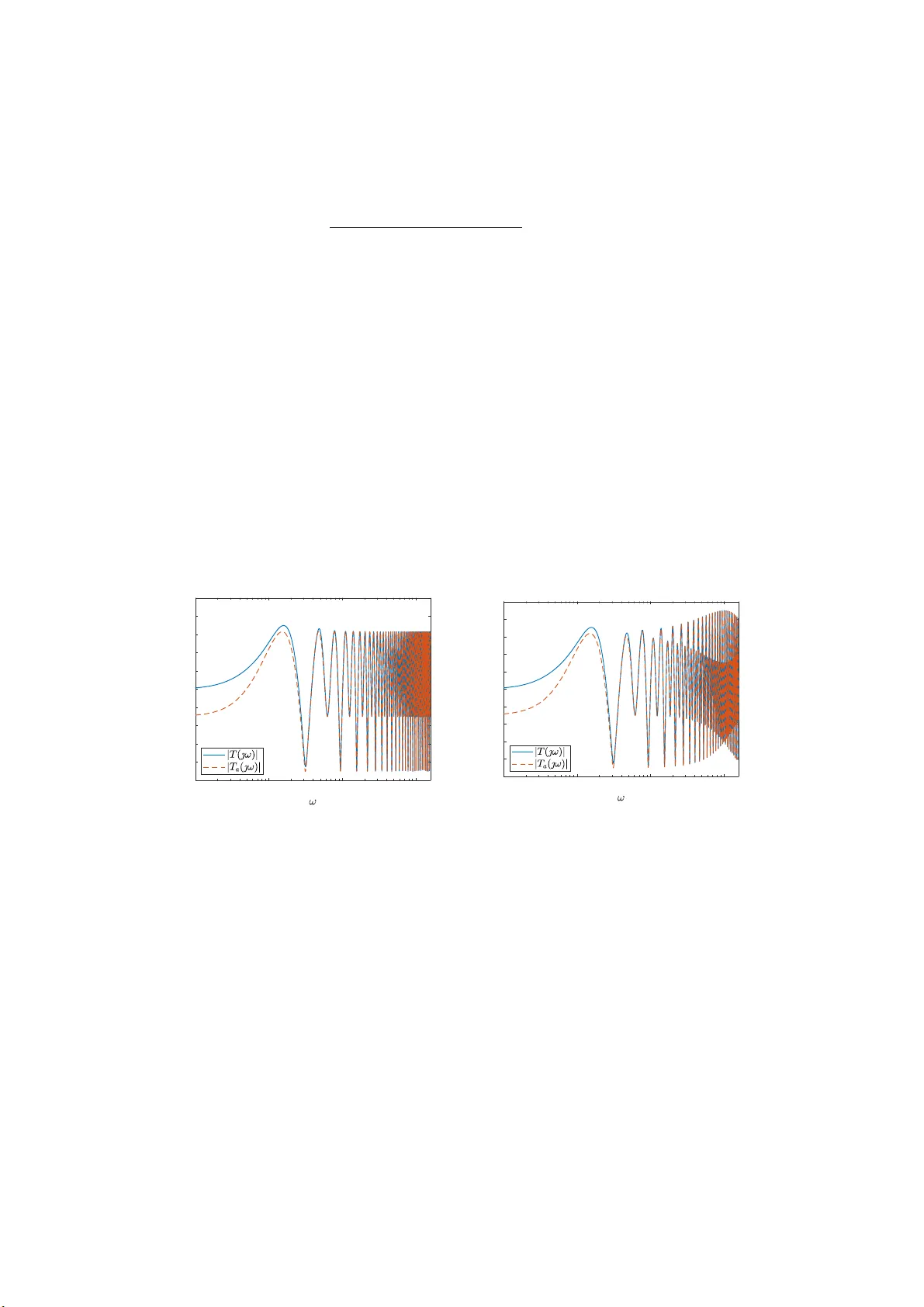
A pseudo-sp ectra based c haracteri sation of the robust strong H-infinit y norm of time-dela y systems with real-v alued and structured uncertain ties Pieter Appeltans and Wim Mic hiels Abstract This pap er examines the robust (strong) H-infinity norm of a linear time-inv arian t system with discrete delays. The considered system is sub ject t o real-va lued, structured, F robenius norm b ounded un certa inties on the co efficie nt matrices. The robust H-infinity norm is the w orst case v alue of the H-infinity norm ov er the realisati ons of the system and hence an imp ortan t measure of robust p erfo rmance i n control engineering. Ho wev er this robust H-infinity norm is a fragile measure, as for a particular realization of th e uncertainties the H - infinity norm might b e sensitiv e to arbitrarily small p erturbations on the delays. Therefore, w e introduce the robust strong H-infinity n o rm, inspired by the notion of strong stabilit y of dela y differential equations of neutral type, whic h takes into account b oth th e p erturbations on the system matrices and infinitesimal small d el ay p erturbations. This quantit y is a con tinuous function of the nominal sy stem parameters and d elays. The main con tribution of th is work is the introduction of a relation b etw een this robust strong H -infinit y norm and the the pseudo-sp ectrum of an asso cia ted singular delay eigen v alue problem. This relation is subsequently employ ed in a nov el algorithm for computing th e robust strong H -infinit y norm of uncertain time-delay systems. Both the theoretical results and the algorithm are also generalized to systems w ith uncertain ties on t he delays, and s y stems describ ed by a class of dela y differen tial algebraic equations. 1 In tro duction In this work we will fo cus on linear, time-in v ariant systems with discrete delays:    ˙ x ( t ) = A 0 x ( t ) + P K k =1 A k x ( t − τ k ) + B 0 w ( t ) + P K k =1 B k w ( t − τ k ) z ( t ) = C 0 x ( t ) + P K k =1 C k x ( t − τ k ) + D 0 w ( t ) + P K k =1 D k w ( t − τ k ) . (1) with x ∈ R n the state, w ∈ R m the exogenous inp ut and z ∈ R p the exogenous output; A k , B k , C k and D k for k = 0 , . . . , K real-v alued sy s tem matrices of appropriate dimension; and ~ τ = ( τ 1 , τ 2 , . . . , τ K ) ∈ ( R + ) K discrete delays. The transfer function asso ciated with this system equals: T ( s ; ~ τ ) =  C 0 + K P k =1 C k e − sτ k   sI − A 0 − K P k =1 A k e − sτ k  − 1  B 0 + K P k =1 B k e − sτ k  + D 0 + K P k =1 D k e − sτ k . The H ∞ -norm is an imp ortant per formance measure of dynamical systems as it quan tifies the disturbance r ejection of the sys tem. It is frequently used in the robust control framework [1]. F or sys tem (1), if exp onen tially stable, the H ∞ -norm is equal to the supremum of the frequency resp onse (ie. the transfer function ev aluated at the ima g inary axis) measured in sp ectral norm: k T ( · ; ~ τ ) k H ∞ = sup ω ∈ R σ 1 ( T ( ω ; ~ τ )) (2) 1 with σ 1 ( · ) the lar gest singular v alue [1]. This quantit y contin uously dep ends o n the elements of the ma trices A k , B k , C k and D k at v alues for which the system is exp onen tially sta ble. Ho wev er the function ~ τ 7→ k T ( · ; ~ τ ) k H ∞ might be discontin uous, even if the system r e ma ins s table. This is caused by the p oten tial sensitivit y of the a symptotic frequency resp o nse, defined as T a ( ω ; ~ τ ) := D 0 + K X k =1 D k e − ω τ k , (3) with respect to infinitesimal small delay changes [2]. R emark 1 . The name asymptotic frequency res ponse stems from the following prop ert y . Prop ert y 1 ([2, Prop osition 3.3]) . It holds that, lim ¯ ω →∞ max n σ 1  T ( ω ) − T a ( ω )  : ω ≥ ¯ ω o = 0 and lim sup ω →∞ σ 1  T ( ω ; ~ τ )  = sup ω ∈ R σ 1  T a ( ω ; ~ τ )  = k T a ( · ; ~ τ ) k H ∞ . T o eliminate this p otent ia l discontin uity with resp ect to the delays, one often w o rks with the strong H ∞ -norm instead: ||| T ( · ; ~ τ ) ||| H ∞ := lim sup γ → 0+  k T ( · ; ~ τ γ ) k H ∞ : ~ τ γ ∈ B ( ~ τ , γ ) ∩ ( R + ) K  , with B ( ~ τ , γ ) a ball with ra dius γ in R K cent r ed a t ~ τ [2]. The stro ng H ∞ -norm of the a symptotic frequency r esponse, ||| T a ( · ; ~ τ ) ||| H ∞ , is defined analogo usly . The stro ng H ∞ -norm of system (1) has the following pr o perties: Prop ert y 2 ([2, Theorem 4.5]) . The strong H ∞ -norm is contin uous as a function of the e lements of the sy stem matrices and the delays at v alues for whic h the system is exp onen tially stable. Prop ert y 3 ([2, Theorem 4.5]) . The strong H ∞ -norm of system (1) satisfies ||| T ( · ; ~ τ ) ||| H ∞ = max  k T ( · ; ~ τ ) k H ∞ , ||| T a ( · ; ~ τ ) ||| H ∞  and ||| T a ( · ; ~ τ ) ||| H ∞ = max ~ θ ∈ [0 , 2 π ) K σ 1 D 0 + K X k =1 D k e θ k ! . (4) Prop ert y 4 ([2, Prop osition 4.3]) . It holds that, ||| T a ( · ; ~ τ ) ||| H ∞ ≥ k T a ( · ; ~ τ ) k H ∞ . F urthermor e, if the delays are rationally independent, then ||| T a ( · ; ~ τ ) ||| H ∞ = k T a ( · ; ~ τ ) k H ∞ and a s a consequence ||| T ( · ; ~ τ ) ||| H ∞ = k T ( · ; ~ τ ) k H ∞ . The following example illustrates the p oten tial s e nsitivit y of the H ∞ -norm with resp ect to infinitesimal dela y changes in greater detail. Example 1. Let us consider the following system ( ˙ x ( t ) = − 2 x ( t ) + x ( t − τ 1 ) − w ( t ) − 0 . 5 w ( t − τ 2 ) z ( t ) = − 2 x ( t ) + x ( t − τ 2 ) +5 w ( t ) +1 . 5 w ( t − τ 1 ) − 3 w ( t − τ 2 ) (5) 2 whose corr esponding tra nsfer function a nd asymptotic frequency resp onse function are resp ec- tiv ely equal to T ( s ; ( τ 1 , τ 2 )) = ( − 2 + e − sτ 2 )( − 1 − 0 . 5 e − sτ 2 ) s + 2 − e − sτ 1 + 5 + 1 . 5 e − sτ 1 − 3 e − sτ 2 and T a ( ω ; ( τ 1 , τ 2 )) = 5 + 1 . 5 e − ω τ 1 − 3 e − ω τ 2 . Figure 1a plots the magnitude of the frequency resp onse and the asymptotic frequency resp onse in function o f ω for τ 1 and τ 2 resp ectiv ely equal to 1 a nd 2 . F or these v alues o f dela ys, the magnitude of the frequency r esponse attains a ma xim um of a ppro xima tely 8 . 4 907 . Figure 1 b shows the effect of a small change in delay parameters ( τ 1 = 1 and τ 2 = 2 + π / 100 ). Now the H ∞ -norm is equal to a ppro ximately 9 . 5 . F ur ther more, from Proper ties 3 and 4 it fo llows that k T ((1 , 2 + π /n )) k H ∞ = ||| T ((1 , 2 + π /n )) ||| H ∞ ≥ ||| T a ((1 , 2 + π/ n )) ||| H ∞ = max ~ θ ∈ [0 , 2 π ) 2 σ 1  5 + 1 . 5 e θ 1 − 3 e θ 2  = 9 . 5 for e v ery n ∈ N . One can thus choose delays ar bit r arily clo se to (1 , 2) for which the H ∞ -norm jumps to at least 9 . 5 . F rom the figures it is also clear that this discontin uit y is due to the asymptotic frequency res p onse. 10 -1 10 0 10 1 10 2 0 1 2 3 4 5 6 7 8 9 10 (a) 10 -1 10 0 10 1 10 2 0 1 2 3 4 5 6 7 8 9 10 (b) Figure 1: The magnitude of the frequency resp onse (blue) and asymptotic frequency resp onse (red) of system (5) in function of ω for ( τ 1 , τ 2 ) equal to (1 , 2) (left) and (1 , 2 + π / 100) (righ t). By considering the stro ng H ∞ -norm we r emo ve a fr agility pro blem of the H ∞ -norm, namely being potentially sens itive to infinitesimal perturbations on the delays. Note that the stro ng H ∞ -norm is still a prop erty of the nominal mo del (and infinitesimal p erturbations o f the delays). How ever, in almost all c on trol desig n applications the mathema tica l mo del do es not completely match the dyna mical system it describ es, due to unmo delled (non-linear ) behaviour, mo del reductions, imprecise measurements or uncertain parameters . T o take these deviations in to account during the design pro cess one often works with a family o f mo dels ins tea d [1, 3]. In this pap er, we cons truct such a family by c onsidering (1) as nominal mo del to which uncertainties are added. In the main part of this work we will consider real-v alued (as the mo del of the system itself is rea l- v a lued) , norm-b ounded (reflecting the dista nce b et ween model and rea lit y) and structured (only a cer tain parameter or g roup of parameters is affected) uncertainties on the co efficien t matrices . Ho wev er in Section 5 a lso uncertainties on the delays will be exa mined. 3 The state-space re pr esen tation a s sociated with the considered uncertain system is equal to:          ˙ x ( t ) = ˜ A 0 ( δ ) x ( t ) + K P k =1 ˜ A k ( δ ) x ( t − τ k ) + ˜ B 0 ( δ ) w ( t ) + K P k =1 ˜ B k ( δ ) w ( t − τ k ) z ( t ) = ˜ C 0 ( δ ) x ( t ) + K P k =1 ˜ C k ( δ ) x ( t − τ k ) + ˜ D 0 ( δ ) w ( t ) + K P k =1 ˜ D k ( δ ) w ( t − τ k ) (6) where the uncertainties δ are confined to a sp ecified set ˆ δ . In this for m ulation x ∈ R n is the state vector, w ∈ R m the exogenous input, z ∈ R p the exogenous output, ~ τ = ( τ 1 , τ 2 , . . . , τ K ) ∈ ( R + ) K discrete delays, δ the combination of all uncer ta in ties: δ = ( δ 1 , . . . , δ L ) , ˆ δ the se t o f admissible uncertainties: ˆ δ = { δ ∈ R q 1 × r 1 × · · · × R q L × r L : k δ l k F ≤ ¯ δ l for l = 1 , . . . , L } , ˜ A k ( δ ) , ˜ B k ( δ ) , ˜ C k ( δ ) , and ˜ D k ( δ ) uncertain system matrices of appropria te dimension with ˜ A k ( δ ) = A k + P L l =1 P S A k l s =1 G A k l,s δ l H A k l,s where G A k l,s and H A k l,s are r e a l-v alued shap e matrices of a ppropriate dimension and ˜ B k ( δ ) , ˜ C k ( δ ) and ˜ D k ( δ ) defined analog ously . Note that this definition allows a single uncertaint y to affect multiple blo c ks in the same syste m matrix and even multiple system matrices as the same uncertain parameter may b e present at multiple lo cations. In the remainder of this work we make the following assumption for this uncertain system: Assumption 1. System (6) is int ernally exp onential ly stable for al l admissible unc ertainties, ie. the char acteristic r o ots of λI − ˜ A 0 ( δ ) − ˜ A k ( δ ) e − λτ k lie in the op en left half plane for al l δ ∈ ˆ δ . F or such uncertain systems it is often desirable to quan tify the worst behaviour ov er all po ssible rea lisations. In the context of the H ∞ -norm this led to the no tion of the robust H ∞ - norm whic h is defined as the maximal H ∞ -norm ov er all realisations , ie. k T ( · ; · , ~ τ ) k ˆ δ H ∞ := max δ ∈ ˆ δ k T ( · ; δ, ~ τ ) k H ∞ where T ( s ; δ, ~ τ ) is the transfer functions asso ciated with a given r ealisation of (6): T ( s ; δ, ~ τ ) =  ˜ C 0 ( δ ) + K P k =1 ˜ C k ( δ ) e − τ k s  I s − ˜ A 0 ( δ ) − K P k =1 ˜ A k ( δ ) e − τ k s  − 1  ˜ B 0 ( δ ) + K P k =1 ˜ B k ( δ ) e − τ k s  + ˜ D 0 ( δ ) + K P k =1 ˜ D k e − τ k s . (7) The robust H ∞ -norm can also b e in ter pr eted as the s uprem um of the following (worst-case ga in) function R ∋ ω 7→ max δ ∈ ˆ δ σ 1  T ( ω ; δ, ~ τ )  ∈ R + , (8) which for each frequency giv es the maximal (ov er b oth the input signals and the admiss ible realisations) input-output gain of the s ystem. How ever, the potential disco n tin uity of the nominal H ∞ -norm with resp ect to the dela ys caries ov er to the robust H ∞ -norm. Therefore this pap er works with the r o bust stro ng H ∞ - norm instead: ||| T ( · ; · , ~ τ ) ||| ˆ δ H ∞ := max δ ∈ ˆ δ ||| T ( · ; δ, ~ τ ) ||| H ∞ which , by Prop ert y 3, is equal to ||| T ( · ; · , ~ τ ) ||| ˆ δ H ∞ = max n max δ ∈ ˆ δ k T ( · ; δ, ~ τ ) k H ∞ | {z } k T ( · ; · ,~ τ ) k ˆ δ H ∞ , max δ ∈ ˆ δ ||| T a ( · ; δ , ~ τ ) ||| H ∞ | {z } ||| T a ( · ; · ,~ τ ) || | ˆ δ H ∞ o . (9) 4 F rom this definition it follows that either ||| T ( · ; · , ~ τ ) ||| ˆ δ H ∞ = ||| T a ( · ; · , ~ τ ) ||| ˆ δ H ∞ or ||| T ( · ; · , ~ τ ) ||| ˆ δ H ∞ = k T ( · ; · , ~ τ ) k ˆ δ H ∞ > ||| T a ( · ; · , ~ τ ) ||| ˆ δ H ∞ . In the former case the robust strong H ∞ -norm is e q ual to the worst-case v alue o f the strong H ∞ -norm of the asy mpt o tic transfer function (which we will cal l the robust s tr ong asymptotic H ∞ -norm in the remainder of this pap er). In the latter ca s e the robust stro ng H ∞ -norm is equal to maximum of the worst-case g ain function (which is attained at finite freq uencie s ). W e comeba c k to this characterisation in Section 3.4. The existing numerical metho ds to c o mpute the nominal H ∞ -norm (of delay fre e systems) can b e divided in tw o classes . A first g roup [4, 5, 2] is based on the BBB S level-set algo rithm presented in [5]. These metho ds r e p eatedly co mput e the sp ectrum of an asso ciated Hamiltonian eigenv a lue pro blem a nd chec k for s tr ictly imaginary (ie. rea l par t eq ual to zer o) eigenv alues. Because the cost of this last ope r ation increases cubica lly with the size of the state matrix, this method is ra ther slow for large systems. The seco nd class [6, 7] avoids this complete eigenv alue decomp osition by us ing the relation b et ween the H ∞ -norm and the structured distance to insta- bilit y (also known a s the stabilit y r adius [3]) of an a ssociated singular eigenv alue pr o blem with a s tructured, complex-v alued p erturbation. Mo re sp ecifically: Prop osition 1 ([6, Propo sition 3.2]) . The H ∞ -norm of T ( s ) = C ( I s − A ) − 1 B + D is equal to the recipro cal of the structured distance to insta bilit y of M ( λ ; ∆) :=   I 0 0 0 0 0 0 0 0   λ −     A B 0 0 − I 0 C D − I   +   0 I 0   ∆  0 0 I    , (10) which is defined as the smallest ǫ such that there exists a ∆ ∈ C m × p with k ∆ k 2 ≤ ǫ for characteristic matrix (10) is not well-po sed (see later on) or has (a) characteristic ro ot(s) in the closed right half pla ne. The main computation cost o f these las t algor ithms stems fro m ca lculating the right-most eigen- v alues of (10) for several ∆ . F or lar ge, s pa rse matrices these rig h t-most eigenv a lues can efficiently be co mput ed using sp ecialised iterative methods such as [8, 9]. The metho d presented in this pap er fits in this last framework. The r emainder of this pap er is organis e d a s follows. In Section 2 we r evise some theory related to (p e r turbed) sing ular delay e ig en v alue pr o blems. Section 3 contains the main theor etical result of the pap er as it gives the relation b et ween the robust strong H ∞ -norm of system (6) and the (robust structured complex) distance to instability of an asso ciated singular delay e ig en v alue problem. Next, Section 4 presents a numerical algorithm, based on this relation, to compute the r o bust strong H ∞ -norm. Subsequently Section 5 gener alises the theor y and the presented method to sy stems with uncertainties on b oth the c o efficient matrices and the delays, and to systems whose nominal mo del is repr esen ted by delay differential a lgebraic equatio ns. Finally , Sections 6 a nd 7 g iv e s ome num er ical examples a nd concluding remarks . 2 Singular dela y eigen v alue problems As mentioned in Prop osition 1, there exists a link betw een the H ∞ -norm of a delay fr e e system and the structured distance to instability of an asso ciated s ingular eigenv a lue problem. Section 3 in tro duces a similar relation b et ween the robust strong H ∞ -norm of system (6) and the (robust structured complex) distance to instability of a singular delay eig en v alue pr o blem (SDEP) whose nominal characteris tic matrix has the following s tr ucture M ( λ ; ~ τ ) := Qλ − P 0 − K X k =1 P k e − λτ k (11) 5 with Q , P 0 , ..., P K square matrices of dimension n M (= n + m + p ) a nd ~ τ = ( τ 1 , τ 2 , . . . , τ K ) ∈ ( R + ) K discrete delays. The matrix Q ca n b e s ingular a nd in the remainder o f this pap er U N and V N will denote n M × ( n M − rank( Q )) -dimensional matric e s who se columns form a basis for resp ectiv ely the le ft and right nullspace of Q . The b ehaviour of such eigenv alue problems is howev er non-trivial. Therefore this section will r evise some related theo r y . Fir s t the fo cus lies on the nominal eigenv alue problem (Section 2.1). Subsequently the effect of structured per turbations is examined (Section 2.2). 2.1 Sp ectral prop erties T o get a b etter understanding of the eigenv alue problem ass ociated with (11), we first examine some proper ties of a singular eigenv alue pr oblem without delays in the characteristic matrix: N ( λ ) := Qλ − P 0 . (12) This ch a racteristic matr ix is called reg ular when its characteristic p olynomial  C ∋ λ 7→ det( N ( λ ))  do es not v anish identically [10]. If (12) is regula r, it ca n be transformed to W eier strass-Kronecker canonical for m [10, 11]: there exist nonsingular matrice s W and T such that W QT =  I µ 0 0 N  and W P 0 T =  J 0 0 I n − µ  with µ the sum of the algebr aic multiplicities of all finite eigenv a lues, J in Jordan form a nd N a nilp oten t matr ix in Jor dan fo rm. The index of (12) is defined as the s mallest int eg er ν such that N ν = 0 (and the index is equal to 0 if N is void). W e now return to o ur origina l SDEP . As in [10], characteristic matrix (11) is said to b e regular if Qλ − P 0 is re g ular a nd (if r e gular) its index is equal to the index o f Qλ − P 0 . Based on these notions o f regular it y a nd index, we present well-posednes s in the remainder o f this work in the following wa y: Definition 1. Characteristic matrix (11) is called well-posed when it is re g ular and has a t most index 1. The followin g lemma allows us to easily v er ify this well-posednes s co ndit io n. Lemma 1 ([12, Lemma 2]) . Char acteristic matrix (11) is wel l-p ose d if and only if U N H P 0 V N is non-singular. Next we re s trict o urself to w ell- posed characteristic matrice s a nd ex amine some prop erties of their (finite) sp ectrum: Λ( ~ τ ) := n λ ∈ C : det( M ( λ ; ~ τ )) = 0 o . (13) Because neutra l dela y eigenv alue pro blems can b e reformulated in for m (11) (see [13]), some prop- erties o f neutral delay eigen v alue problems carry over to the studied SDEPs. More sp ecifically the spectra l abscissa o f (13), ie. α ( ~ τ ) := sup {ℜ ( λ ) : λ ∈ Λ ( ~ τ ) } , may b e dis c o n tinuous with resp ect to the delays. W e therefore co nsider the strong spec tr al abscissa [13]: α s ( ~ τ ) := lim sup γ → 0+ { α ( ~ τ γ ) : ~ τ γ ∈ B ( ~ τ , γ ) ∩ ( R + ) K } , which has the following prop erty . Prop ert y 5 ([13, Prop ostition 3]) . The strong spectra l abscissa satisfies α s ( ~ τ ) = ma x n α D,s ( ~ τ ) , α ( ~ τ ) o 6 with α D,s ( ~ τ ) equal to the zero cr ossing of R ∋ ς 7→ max ~ θ ∈ [0 , 2 π ) K ρ K X k =1  U N H P 0 V N  − 1  U N H P k V N  e − ς τ k + θ k ! − 1 , (14) where ρ ( · ) is the sp ectral r a dius, if such a crossing exists and otherwise α D,s ( ~ τ ) = − ∞ . In addi- tion, the strong spectra l absciss a is contin uous with r espect to b o th the elements of P 0 , . . . , P K and the delays ~ τ as long as U N H P 0 V N remains non- s ingular. Finally , we in tro duce the following definition of s trong stability based on the notions of well- po sedness and strong spectra l abscissa. Definition 2. A characteristic matrix M ( λ ; ~ τ ) is strong ly stable if it is well-po sed and its strong sp e ctral abscissa is strictly nega tiv e. 2.2 Robust structured complex distance to instabilit y This subsection examines the effect of adding p erturbations to a stro ngly stable characteristic matrix. Inspired by Prop osition 1, we fo cus on a characteris tic matrix of the follo wing form: M ( λ ; δ, ∆ , ~ τ ) :=   I n 0 0 0 0 0 0 0 0   | {z } Q λ −   ˜ A 0 ( δ ) ˜ B 0 ( δ ) 0 0 − I m 0 ˜ C 0 ( δ ) ˜ D 0 ( δ ) − I p   −   0 I m 0   ∆  0 0 I p  | {z } ˜ P 0 ( δ , ∆ ) − K X k =1   ˜ A k ( δ ) ˜ B k ( δ ) 0 0 0 0 ˜ C k ( δ ) ˜ D k ( δ ) 0   | {z } ˜ P k ( δ ) e − λτ k , (15) with ˜ A k , ˜ B k , ˜ C k , ˜ D k and ~ τ a s defined in Section 1 and ∆ ∈ C m × p . Observe that characteristic matrix (15) shares some similarities with (1 0). But there a r e tw o main differences: firstly (15) contains delay terms (due to the discr e te delays in (6)) a nd seco ndly (15) has b oth real- a nd complex-v alued p erturbations. The r eal-v alued p erturbations ( δ ) or iginate fro m the uncertainties in mo del (6) and ar e therefore co nfined to the set ˆ δ . The complex v alued p erturbation ( ∆ ) on the other hand plays a similar role as in Propo sition 1: we ar e in ter e sted in the smallest ǫ such that there exists a ∆ ∈ C m × p with k ∆ k 2 ≤ ǫ for which M ( λ ; δ, ∆ , ~ τ ) is not strongly stable for at least o ne δ ∈ ˆ δ . This critical ǫ will b e called the r obust (worst-case v alue o ver all p ermissible real-v alued p erturbations) structured c omplex (to emphasise that only the b ound on the complex- v alued p erturbation is v aried) distance to insta bility . In Section 3 it will b e shown that there exists a relation betw een this ro bust structured co mplex distance to instability and the robust strong H ∞ -norm o f system (6), while in the remainder of this subse c tion we c ha racterise this robust structured complex distance to insta bility in greater detail. F rom the definition of s trong s tabilit y (see Definition 2), it follows that ther e are t wo wa ys in which a loss of strong stability can o ccur. Fir stly , the characteristic matrix can b ecome non well- po sed. The corres ponding robust structured complex distance to no n w ell- p osedness is defined as: dist N W P ( ˆ δ ) =    + ∞ , if M ( λ ; δ, ∆ , ~ τ ) is w ell- p osed for all ∆ ∈ C m × p and δ ∈ ˆ δ min δ ∈ ˆ δ ∆ ∈ C m × p {k ∆ k 2 : M ( λ ; δ, ∆ , ~ τ ) is not w ell-p osed } , otherwise . ( 1 6) Secondly , a realisa tion of (15) can lo ose s tr ong s tabilit y if its strong sp ectral abscissa b ecomes non-negative. Therefor e we study the ( ˆ δ , ǫ ) -strong pseudo -spectral a bscissa of (15) , which for ǫ ∈ [0 , dist N W P ) is defined as the maximal stro ng sp ectral abscissa over a ll r ealisations of (15) with δ ∈ ˆ δ and k ∆ k 2 ≤ ǫ : α ps s ( ˆ δ , ǫ , ~ τ ) := max δ ∈ ˆ δ max ∆ ∈ C m × p k ∆ k 2 ≤ ǫ α s ( δ, ∆ , ~ τ ) 7 with α s ( δ, ∆ , ~ τ ) the str ong spectr al abscissa of M ( λ ; δ, ∆ , τ ) . Using Pro perty 5 this leads to α ps s ( ˆ δ , ǫ, ~ τ ) = max  max δ ∈ ˆ δ max ∆ ∈ C m × p k ∆ k 2 ≤ ǫ α D,s ( δ, ∆ , ~ τ ) | {z } α ps D,s ( ˆ δ ,ǫ,~ τ ) , max δ ∈ ˆ δ max ∆ ∈ C m × p k ∆ k 2 ≤ ǫ α ( δ, ∆ , ~ τ ) | {z } α ps ( ˆ δ, ǫ , ~ τ )  . (17) R emark 2 . The v alue α ps ( ˆ δ , ǫ , ~ τ ) can b e interpreted as the supremum of the r e al par t of the po in ts in the ( ˆ δ , ǫ ) -pseudo-sp ectrum o f (15), ie. α ps ( ˆ δ , ǫ , ~ τ ) = sup {ℜ ( λ ) : λ ∈ Λ ps ( ˆ δ , ǫ , ~ τ ) } with Λ ps ( ˆ δ , ǫ , ~ τ ) = [ δ ∈ ˆ δ [ ∆ ∈ C m × p k ∆ k 2 ≤ ǫ  λ ∈ C : det  M ( λ ; δ , ∆ , ~ τ )  = 0  . (18) Based on (17) w e now introduce tw o other distance measures. Firs tly , the r obust structured complex dis tance to a characteristic roo t chain cro ssing is defined as dist C H AI N ( ˆ δ ) = ( + ∞ , if α ps D,s ( ˆ δ , ǫ, ~ τ ) < 0 ∀ ǫ ∈ [0 , dist N W P ) min { ε ∈ [0 , dist N W P ) : α ps D,s ( ˆ δ , ǫ , ~ τ ) ≥ 0 } , otherwise . (19) Secondly , the robust structure d complex distance to finite ro ot cro ssing is defined as dist F I N ( ˆ δ ) = ( + ∞ , if α ps ( ˆ δ , ǫ, ~ τ ) < 0 ∀ ǫ ∈ [0 , min { dist N W P , dist C H AI N } ) min { ǫ ∈ [0 , min { dist N W P , dist C H AI N } ) : α ps ( ˆ δ , ǫ , ~ τ ) ≥ 0 } , otherwise . ( 2 0) The names of these t wo distances can be understo o d using the following pr operty . Prop ert y 6. [14] If α D,s ( ~ τ ) ≥ 0 then for ea c h γ > 0 there exist ~ τ γ ∈ B ( ~ τ , γ ) ∩ ( R + ) K and c ≥ 0 such that Λ( ~ τ γ ) con tains a c hain of characteristic ro ots { λ i } i ∈ N that satisfies lim i →∞ ℜ ( λ i ) = c lim i →∞ |ℑ ( λ i ) | = + ∞ . If α D,s ( ~ τ ) < 0 , ther e exist ǫ 1 > 0 and ǫ 2 > 0 such that for a n y ~ τ ǫ 1 ∈ B ( ~ τ , ǫ 1 ) ∩ ( R + ) K the num b er of c ha r acteristic r oots of M ( λ ; ~ τ ǫ 1 ) that lie to the r igh t o f − ǫ 2 is finite. A finite robus t s tructured complex dista nce to a c har acteristic ro ot chain cro ssing is thus the smallest ǫ fo r which there ex is t δ ∈ ˆ δ and ∆ ∈ C m × p with k ∆ k 2 ≤ ǫ such that the s pectrum o f the asso ciated realisatio n of (15) contains a chain of characteristic ro ots with a vertical asymptote in the clos ed right-half plane, for some delays ~ τ γ that can b e chosen arbitrar ily close to ~ τ . At the same time a finite r o bust structured co mplex distance to finite ro ot c r ossing corr esponds to the smallest ǫ for which there exists δ ∈ ˆ δ and ∆ ∈ C m × p with k ∆ k 2 ≤ ǫ such that the sp e ctrum of M ( λ ; δ, ∆ , ~ τ ) has (finitely many) eige nv alues in the close d righ t half pla ne (note that for ǫ < dist C H AI N ( ˆ δ ) the n umber o f r o ots in the clo sed rig h t-half plane is finite, even for infinitesimal small delay p erturbations). Thes e co ncepts are illustrated in Exa mples 2, 3 and 4 in Section 3. R emark 3 . Because the str ong sp ectral abscissa of a given r ealisation of (15) is contin uous with resp ect to the elemen ts of ∆ as long as k ∆ k 2 < dist N W P (a consequence of Prop erty 5), a transition to a no n-negativ e ps e udo -spectral abscissa is character ised by a c r itical ǫ ⋆ for which α ps s ( ˆ δ , ǫ ⋆ , ~ τ ) = 0 . The r obust structured complex distance to instability now can b e e x pressed in function of the three distance measures defined a bov e: dist I N S ( ˆ δ ) = min n dist N W P ( ˆ δ ) , dist C H AI N ( ˆ δ ) , dist F I N ( ˆ δ ) o . (21) 8 3 Relation b et w een the robust strong H ∞ -norm and the ro- bust structur ed com pl ex distance to instabilit y This section esta blishes the relatio n betw een the robust str ong H ∞ -norm of system (6) and the robust structur ed complex distance to instability of (15). Section 3.1 gives so me preliminary results. In Section 3.2 w e fo cus on the relation b et ween the ro bust strong asymptotic H ∞ - norm a nd the robust structured co mplex distances to non well-po sedness and characteristic r oot chain cros s ing. Next, Section 3.3 inv estiga tes the link b et ween the worst-case ga in function at finite frequencies a nd the robust s tructured complex distance to finite ro ot cr ossing. Finally , Section 3.4 combines these results and gives s ome examples. 3.1 Preliminary results W e start with so me tec hnica l lemmas. Lemma 2. F or a matrix A ∈ C p × m it holds that σ 1 ( A ) − 1 = min ∆ ∈ C m × p {k ∆ k 2 : det ( I m − ∆ A ) = 0 } and σ 1 ( A ) − 1 v u H ∈ argmin ∆ ∈ C m × p {k ∆ k 2 : det ( I m − ∆ A ) = 0 } . wher e u and v ar e re sp e ctively t he left and right singular ve ctors of A asso ciate d with σ 1 ( A ) , the lar gest singular value of A . Pr o of. See for example [15]. Lemma 3. The r obust stru ctur e d c omplex distanc e to instability of (15) is non-zer o if and only if the char acteristic r o ots of I λ − ˜ A 0 ( δ ) − P K k =1 ˜ A k ( δ ) e − λτ k lie in the op en left half-plane for al l δ ∈ ˆ δ . Pr o of. B e cause U N H ˜ P 0 ( δ, 0 m × p ) V N =  − I 0 ˜ D 0 ( δ ) − I  is no n- singular for a ll δ ∈ ˆ δ , it follows from Lemma 1 that the ro bust structured complex distance to non well-po sedness is non-zero. F urther more, it is ea s y to verify that α ps D,s ( ˆ δ , 0 , ~ τ ) = −∞ and thus also the robust structured co mplex distance to a ro ot chain crossing is non zero. Finally , one c a n show that α ps ( ˆ δ , 0 , ~ τ ) = max λ ∈ C ( ℜ ( λ ) : ∃ δ ∈ ˆ δ such that det I λ − ˜ A 0 ( δ ) − K X k =1 ˜ A k ( δ ) e − λτ k ! = 0 ) , from which the lemma follows. By Assumption 1 this means that all characteristic matrices examined in the remainder of this paper hav e a p ositive, non-zero robust structured complex distance to instability . Lemma 4. Assume that the c omplex numb er s is not a char acteristic r o o t of I λ − ˜ A 0 ( δ ⋆ ) − P K k =1 ˜ A k ( δ ⋆ ) e − λτ k . Ther e exists a ∆ ∈ C m × p with k ∆ k 2 ≤ ǫ su ch t ha t s is a char acteristic r o ot of M ( λ ; δ ⋆ , ∆ , ~ τ ) if and only if σ 1  T ( s ; δ ⋆ , ~ τ )  ≥ ǫ − 1 . F urthermor e, s is a char acteristic r o ot of M ( λ ; δ ⋆ , σ 1  T ( s ; δ ∗ , ~ τ )  − 1 v u H , ~ τ ) , wher e u and v ar e r esp e ctively the left and right singular ve ctors of T ( s ; δ ∗ , ~ τ ) asso ciate d with its lar gest singular value. 9 Pr o of. A complex num ber s is a characteris tic ro ot of M ( λ ; δ ⋆ , ∆ , ~ τ ) if and only if det  M ( s ; δ ⋆ , ∆ , ~ τ )  = det               I s − ˜ A 0 ( δ ⋆ ) − K P k =1 ˜ A k ( δ ⋆ ) e − sτ k − ˜ B 0 ( δ ⋆ ) − K P k =1 ˜ B k ( δ ⋆ ) e − sτ k 0 0 I − ∆ − ˜ C 0 ( δ ⋆ ) − K P k =1 ˜ C k ( δ ⋆ ) e − sτ k − ˜ D 0 ( δ ⋆ ) − K P k =1 ˜ D k ( δ ⋆ ) e − sτ k I               = 0 . Because sI − ˜ A 0 ( δ ⋆ ) − P K k =1 ˜ A k ( δ ⋆ ) e − sτ is inv er tible, this last express ion can b e rewritten, using Sch ur’s deter minan t lemma for blo c k partitioned matr ices, in the following form: det  I − ∆ − T ( s ; δ ⋆ , ~ τ ) I  = det ( I − ∆ T ( s ; δ ⋆ , ~ τ )) = 0 . F rom Lemma 2 it follows that there exists a ∆ ∈ C m × p with k ∆ k 2 ≤ ǫ such that this co ndit io n is met if and only if  σ 1 ( T ( s ; δ ⋆ , ~ τ ))  − 1 ≤ ǫ . And if this la st condition is met, it follows from the second pa rt of Lemma 2 than o ne can cho ose ∆ = σ 1  T ( s ; δ ∗ , ~ τ )  − 1 v u H . 3.2 Link b et w een the asymptotic transfer function and t he r o bu st structured complex distances to non w ell-p osedness and c harac- teristic root c hain crossing W e star t with a characterisation of the robust structure d complex distance to non well-posedness in terms of the delay free direc t feed-through ter m of system (6). Prop osition 2 . It holds that dist − 1 N W P ( ˆ δ ) = max δ ∈ ˆ δ n σ 1  ˜ D 0 ( δ ) o . Pr o of. It follows fro m Lemma 1 that characteristic matrix (15) is non well-posed if and only if U N H  ˜ P 0 ( δ, ∆)  V N =  − I ∆ ˜ D 0 ( δ ) − I  is singular. Using the Sch ur-B a nac hiewicz inv ersion for m ula for block partitioned ma trices, we c a n rewrite this condition as: Chara cteristic matr ix (15) is non well-posed if and only if I − ∆ ˜ D 0 ( δ ) is singular. The robust structured complex distance to non well-posednes s is thus equal to dist N W P ( δ ) =      + ∞ , det  I − ∆ ˜ D 0 ( δ )  6 = 0 for a ll ∆ ∈ C m × p and δ ∈ ˆ δ min δ ∈ ˆ δ ∆ ∈ C m × p {k ∆ k 2 : det  I − ∆ ˜ D 0 ( δ )  = 0 } , otherwise Using Lemma 2, one finds dist N W P ( δ ) =      + ∞ σ 1  ˜ D 0 ( δ )  = 0 for a ll δ ∈ ˆ δ min δ ∈ ˆ δ  σ 1  ˜ D 0 ( δ )  − 1  otherwise =      + ∞ σ 1  ˜ D 0 ( δ )  = 0 for a ll δ ∈ ˆ δ  max δ ∈ ˆ δ n σ 1  ˜ D 0 ( δ ) o  − 1 otherwise 10 Next we derive a c o ndition for a finite robust structured complex distance to a characteristic ro ot chain cross ing in terms of the robust strong a symptotic H ∞ -norm of system (6). Lemma 5. The r obust st ructur e d c omplex distanc e to a char acteristic r o ot chain cr ossing of (15) is finite if and only if max δ ∈ ˆ δ n σ 1  ˜ D 0 ( δ ) o < ||| T a ( · ; · , ~ τ ) ||| ˆ δ H ∞ Pr o of. B y Proper t y 5 and under Assumption 1, the robust structured co mplex distance to a characteristic ro ot chain cro s sing of (15) is finite, if and only if there exist δ ⋆ ∈ ˆ δ , ~ θ ⋆ ∈ [0 , 2 π ) K and ∆ ⋆ ∈ C m × p with k ∆ ⋆ k 2 < dist N W P such that det I + K X k =1  U N H ˜ P 0 ( δ ⋆ , ∆ ⋆ ) V N  − 1 U N H ˜ P k ( δ ⋆ ) V N e θ ⋆ k ! = 0 . Because U N H ˜ P 0 ( δ ⋆ , ∆ ⋆ ) V N is non- s ingular ( k ∆ ⋆ k 2 < dist N W P ), this last condition is equiv alen t with det U N H ˜ P 0 ( δ ⋆ , ∆ ⋆ ) V N + K X k =1 U N H ˜ P k ( δ ⋆ ) V N e θ ⋆ k ! = 0 . Plugging in the definitions of ˜ P 0 , . . . , ˜ P k and using Sch ur’s deter minan t lemma for blo c k parti- tioned matrices the right hand side of the condition reduces to: there exist δ ⋆ ∈ ˆ δ , ~ θ ⋆ ∈ [0 , 2 π ) K and ∆ ⋆ with k ∆ ⋆ k 2 < dist N W P such that det I − ∆ ⋆ ˜ D 0 ( δ ⋆ ) + K X k =1 ˜ D k ( δ ⋆ ) e θ ⋆ k !! = 0 . The lemma follows fro m (4), Le mm a 2 and Propo sition 2 . The following lemma gives a low er b ound for the robust strong a symptotic H ∞ -norm. Lemma 6. It holds that max δ ∈ ˆ δ n σ 1  ˜ D 0 ( δ ) o ≤ ma x δ ∈ ˆ δ max θ ∈ [0 , 2 π ) K ( σ 1 ˜ D 0 ( δ ) + K X k =1 ˜ D k ( δ ) e θ k !) = ||| T a ( · ; · , ~ τ ) ||| ˆ δ H ∞ . Pr o of. Co nsider the matr ix-v alued function C ∋ s 7→ D 0 + P K k =1 D k e − s ∈ C p × m , of which every ent r y is analytic and b ounded for ℜ ( s ) ≥ 0 . F rom [1 6 ] it follo ws that s 7→ σ 1 ( D 0 + P K k =1 D k e − s ) attains it maximum over the closed right-halfplane on ℜ ( s ) = 0 . And th us σ 1 ( D 0 ) = lim s →∞ σ 1 D 0 + K X k =1 D k e − s ! ≤ ma x ω ∈ R σ 1 D 0 + K X k =1 D k e − ω ! ≤ ma x θ ∈ [0 , 2 π ) K σ 1 D 0 + K X k =1 D k e θ k ! . By combining these results we get a n ex pr ession for the robust s trong asymptotic H ∞ -norm in terms o f the robust structured distances to no n well-p osedness and a characteristic r oot ch a in crossing. Prop osition 3. The r obust strong a symptotic H ∞ -norm of (6) is equal to the r eciproca l of the minimum of the ro bust str uctu r ed complex distance to no n w ell-p osedness and the r obust structured c omplex distance to a characteristic ro ot chain cr ossing, ie. ||| T a ( · ; · , ~ τ ) ||| ˆ δ H ∞ = min { dist N W P ( ˆ δ ) , dist C H AI N ( ˆ δ ) } − 1 . 11 Pr o of. Fir st w e consider the cas e wher e dis t C H AI N ( ˆ δ ) < dist N W P ( ˆ δ ) . Using a similar idea a s in the pr oof of Lemma 5 it can be shown that for ǫ ∈ [0 , dist N W P ( ˆ δ )) α ps D,s ( ˆ δ , ǫ , ~ τ ) ≥ 0 if and only if ||| T a ( · ; · , ~ τ ) ||| ˆ δ H ∞ ≥ ǫ − 1 . The smallest ǫ such this last condition is fulfilled is equal to ||| ˜ T a ( · ; · , ~ τ ) ||| ˆ δ H − 1 and thus ||| ˜ T a ( · ; · , ~ τ ) ||| ˆ δ H = dis t C H AI N ( ˆ δ ) − 1 . N ext we consider the cas e where the robust structured complex distance to a characteris- tic roo t chain c r ossing is not finite. It follows from Lemma 5 that max δ ∈ ˆ δ n σ 1  ˜ D 0 ( δ ) o ≥ ||| T a ( · ; · , ~ τ ) ||| ˆ δ H ∞ . But by Lemma 6 we hav e max δ ∈ ˆ δ n σ 1  ˜ D 0 ( δ ) o ≤ ||| T a ( · ; · , ~ τ ) ||| ˆ δ H ∞ . Th us in this case ||| T a ( · ; · , ~ τ ) ||| ˆ δ H ∞ = max δ ∈ ˆ δ n σ 1  ˜ D 0 ( δ ) o = dist N W P ( ˆ δ ) − 1 . 3.3 Link b et w een the worst-case gain function at finite frequencies and the robust structured complex distance to finite ro ot cr ossing The previous subsection established a relation betw een the robust strong asymptotic H ∞ -norm and the robust structured complex distances to non w ell-p osedness and a characteristic ro ot chain cros s ing. In this subsection the link be tw een the worst-cas e gain function (as defined in (8)) and the robust structured complex distance to finite ro ot cr ossing is examined. Lemma 7. The r obust structur e d c omplex distanc e t o finite r o ot cr ossing is finite if and only if system (6 ) attains its ro bust str ong H ∞ -norm at a finite fr e quency (ie. || T ( · ; · , ~ τ ) || ˆ δ H ∞ > ||| T a ( · ; · , ~ τ ) ||| ˆ δ H ∞ ). In such a c ase it holds ||| T ( · ; · , ~ τ ) ||| ˆ δ H ∞ = k T ( · ; · , ~ τ ) k ˆ δ H ∞ = dis t − 1 F I N ( ˆ δ ) . Pr o of. ⇒ It follows fro m Remark 3 a nd Assumption 1 that if the robust structured complex distance to finite ro ot crossing is finite, there e x ist δ ⋆ ∈ ˆ δ , ∆ ⋆ ∈ C m × p with k ∆ ⋆ k 2 ≤ dist F I N ( ˆ δ ) and a finite ω ∈ R s uch that ω is a characteristic ro ot of M ( λ ; δ ⋆ , ∆ ⋆ , ~ τ ) . By Lemma 4, this means that σ 1 ( T ( ω ; δ ⋆ , ~ τ )) ≥ (dist F I N ( ˆ δ )) − 1 >  min { dist N W P ( ˆ δ ) , dist C H AI N ( ˆ δ ) }  − 1 . Using Prop osition 3 one finds that k T ( · ; · , ~ τ ) k ˆ δ H ∞ ≥ σ 1 ( T ( ω ; δ ⋆ , ~ τ )) > ||| T a ( · ; · , ~ τ ) ||| ˆ δ H ∞ . ⇐ If the robust strong H ∞ -norm is attained at a finite frequency then there exists δ ∈ ˆ δ and ω ∈ R such that σ 1 ( T ( ω ; δ, ~ τ )) > ||| T a ( · ; · , ~ τ ) ||| ˆ δ H ∞ . F rom Lemma 4 and Prop osition 3 it follows that there exists a ∆ with k ∆ k 2 = σ 1 ( T ( ω ; δ, ~ τ )) − 1 < min n dist N W P ( ˆ δ ) , dist C H AI N ( ˆ δ ) o such that c har acteristic matr ix M ( λ ; δ, ∆ , ~ τ ) has a characteristic ro ot at ω . k T ( · ; · , ~ τ ) k ˆ δ H ∞ = dist F I N ( ˆ δ ) − 1 is found using Lemma 4 and by maximising σ 1 ( T ( ω ; δ, ~ τ )) over all δ ∈ ˆ δ and ω ∈ R . 12 3.4 Main theoretical result In this subsection the results of the t wo pr e vious subsections are co m bined to characterise the robust strong H ∞ -norm in ter ms of the ro bust structured complex distance to instability . Sub- sequently some e x amples are given. Theorem 1. The r obust str ong H ∞ -norm of an internal ly exp onential ly st a ble system of form (6) is e qual to the r e cipr o c a l of the r obust stru ctur e d c omplex distanc e to instability of char acter- istic matrix (1 5) , ie. ||| T ( · ; · , ~ τ ) ||| ˆ δ H ∞ = 1 dist I N S ( ˆ δ ) Pr o of. If the r obust strong H ∞ -norm is attained at finite fr e q uencies then the res ult follows from Lemma 7 . Otherwise the r esult follows fro m Prop osition 3. As mentioned in Section 1, the robust strong H ∞ -norm of s ystem (6) is either equal to the robust strong a symptotic H ∞ -norm or to the maximum o f the w o r st-case g ain function. In Section 3 .2 it was shown that the former is r elated to the robust structured complex distances to non well-po sedness a nd a characteristic ro o t chain cross ing. Section 3.3 proved that the latter relates with the robust structured c o mplex distance to finite r oot crossing. The following examples illustrate this duality in more detail. Example 2. In this first exa mple w e consider the follo wing uncertain sys tem ( ˙ x ( t ) = ( − 7 + 3 δ 1 ) x ( t ) + ( − 5 + 2 δ 2 ) x ( t − 1) + 4 w ( t ) z ( t ) = (2 − 2 δ 2 ) x ( t ) + (1 + δ 1 ) w ( t ) + w ( t − 1) (22) where δ 1 and δ 2 are r espectively co nfined to | δ 1 | ≤ 0 . 1 5 and | δ 2 | ≤ 0 . 2 , and its corres p onding characteristic matrix:   λ 0 0 0 0 0 0 0 0   −   ( − 7 + 3 δ 1 ) 4 0 0 − 1 ∆ (2 − 2 δ 2 ) (1 + δ 1 ) − 1   −   ( − 5 + 2 δ 2 ) 0 0 0 0 0 0 1 0   e − λ . (23) First we exa mine the ro bust structur e d complex distance to instability of (23). Subsequently , we illustrate the relation of this distance measur e with the be haviour o f system (22). Prop osition 2 gives us a n expr ession for the robust structured complex distance to non well- po sedness: dist N W P ( ˆ δ ) =  max | δ 1 |≤ 0 . 15 | 1 + δ 1 |  − 1 = 1 / 1 . 15 = 0 . 8696 . T o find the ro bust structured complex distance s to a characteristic ro ot chain crossing and finite ro ot crossing we plot α ps ( ˆ δ , ǫ , ~ τ ) and α ps D,s ( ˆ δ , ǫ , ~ τ ) as a function o f ǫ  for ǫ < dist N W P ( ˆ δ )  in Figure 2: dist C H AI N ( ˆ δ ) = 0 . 4651 dist F I N ( ˆ δ ) = 0 . 1663 . The robust structured co mplex distance to insta bility is th us equal to 0 . 1663 and the loss of strong stability is ca used by a finite num b er of characteristic ro ots moving into the closed right- half plane. This is illustrated in Figures 3 and 4. Figure 3 shows the sp ectrum of (23) for the per turbations asso ciated with the loss of strong stability and Figur e 4 shows its ( ˆ δ , ǫ ) -pseudo- sp e ctrum for ǫ smaller than, eq ual to , and lar ger than the distance to insta bilit y . W e observe that the loss of s trong stability is caused by characteristic ro ots moving int o the clo sed rig h t-half plane at s = ±  2 . 734 . 13 Next, we examine how these distance measures re la te to the ro bust strong H ∞ -norm of system (22). The robust strong a symptotic H ∞ -norm follows fro m (4): ||| T a ( · ; · , ~ τ ) ||| ˆ δ H ∞ = max | δ 1 |≤ 0 . 15 max θ ∈ [0 , 2 π )    (1 + δ 1 ) + 1 e θ    = 2 . 15  = min { dist N W P ( ˆ δ ) , dist C H AI N ( ˆ δ ) } − 1  . Figure 5 plo ts the worst-case g ain function. This function attains a ma xim um v alue of 6 . 012 ( = dist F I N ( ˆ δ ) − 1 , indicated in mage nta) at a finite frequency ( ω = 2 . 734 ). F urthermore, for this example the robust strong asymptotic H ∞ -norm can also be deduced from this worst-case gain function (indicated in red) as the system has only one delay which means that: ||| T a ( · ; · , ~ τ ) ||| ˆ δ H ∞ = k T a ( · ; · , ~ τ ) k ˆ δ H ∞ = lim sup ω →∞ max δ ∈ ˆ δ σ 1  T ( ω ; δ, ~ τ )  = 2 . 15 . The robust s trong H ∞ -norm is thus eq ua l to 6 . 01 2 and is equal to the maximum o f the worst-case gain functions. O n figur e 5 we ha ve also indicated dist N W P ( ˆ δ ) − 1 = max δ ∈ ˆ δ n σ 1  ˜ D 0 ( δ ) o . O ne observes that as ω go es to infinity , the worst-case gain function oscillates ar o und this v alue. 0.1 0.15 0.2 0.25 0.3 0.35 0.4 0.45 0.5 -2.5 -2 -1.5 -1 -0.5 0 0.5 Figure 2: α ps ( ˆ δ , ǫ , ~ τ ) (blue) a nd α ps D,s ( ˆ δ , ǫ, ~ τ ) (red) of characteristic matrix (23) in function of ǫ . -2 -1.5 -1 -0.5 0 -60 -40 -20 0 20 40 60 Figure 3: The sp ectrum of characteristic ma- trix (23) for the per turbations asso ciated with the loss o f strong sta bility: ∆ = 0 . 1 663 e  0 . 4065 , δ 1 = 0 . 15 and δ 2 = − 0 . 2 . Example 3. Next we consider the following uncertain system:  ˙ x ( t ) = ( − 3 + δ 2 ) x ( t ) + ( − 1 + 3 δ 1 ) x ( t − 1) + 4 w ( t ) z ( t ) = ( − 2 − 3 δ 1 + 2 δ 2 ) x ( t ) + (3 + δ 1 ) w ( t ) + (1 + δ 1 + δ 2 ) w ( t − 1) (24) where δ 1 and δ 2 are resp ectiv ely confined to | δ 1 | ≤ 0 . 1 and | δ 2 | ≤ 0 . 25 , and its asso ciated characteristic matrix:   λ 0 0 0 0 0 0 0 0   −   − 3 + δ 2 4 0 0 − 1 ∆ − 2 − 3 δ 1 + 2 δ 2 3 + δ 1 − 1   −   − 1 + 3 δ 1 0 0 0 0 0 0 1 + δ 1 + δ 2 0   e − λ . (25) As befo r e, we firs t examine the robust structured complex distance to instability of (25). The robust structured complex distance to no n w ell- p osedness follows from Prop osition 2: dist N W P =  max | δ 1 |≤ 0 . 1 | 3 + δ 1 |  − 1 = 1 / 3 . 1 = 0 . 3 226 . 14 -4 -3.5 -3 -2.5 -2 -1.5 -1 -0.5 0 0.5 -10 -8 -6 -4 -2 0 2 4 6 8 10 -0.7 -0.6 -0.5 -0.4 -0.3 -0.2 -0.1 0 0.1 2.5 2.6 2.7 2.8 2.9 3 3.1 Figure 4: The ( ˆ δ , ǫ ) -pseudo-sp ectrum of characteristic matrix (23) for ǫ equal to 0 . 1429 (gr een dot dash line), 0 . 16 6 3 (blue full line) and 0 . 2 (red dashed line). 10 -1 10 0 10 1 10 2 0 1 2 3 4 5 6 7 Figure 5 : The worst-case gain function of system (22) (blue), || T ( · ; · , ~ τ ) || ˆ δ H ∞ (magenta dot- dashed), ||| T a ( · ; · , ~ τ ) ||| ˆ δ H ∞ (= k T a ( · ; · , ~ τ ) k ˆ δ H ∞ ) (red dashed) and dist N W P ( ˆ δ ) − 1 (green dotted). 15 The robust structured complex distances to a characteristic ro ot c ha in cr ossing and finite ro ot crossing follow from Figure 6: dist C H AI N ( ˆ δ ) = 0 . 2247 dist F I N ( ˆ δ ) = + ∞ . Hence, the robust structured complex distance to instability is equa l to 0 . 22 47 and the loss o f strong s ta bilit y is caused b y a chain of characteristic ro ots who s e vertical asy mpt o te moves into the closed right-half plane. This is illustrated in Figure 7 which shows the spectr um of (25) for the pe r turbations a ssociated with α ps D,s ( ˆ δ , ǫ, ~ τ ) a nd ǫ smaller tha n, equal to and larger than the robust structured complex distance to insta bility . Figure 8 shows the worst-case gain function of system (24). In contrast to the previous ex- ample, it attains its maxima l v alue (of 4 . 45 ) o nly at infinity , ie. k T ( · ; · , ~ τ ) k ˆ δ H ∞ = k T a ( · ; · , ~ τ ) k ˆ δ H ∞ . F urthermor e, as in the previous example k T a ( · ; · , ~ τ ) k ˆ δ H ∞ and ||| T a ( · ; · , ~ τ ) ||| ˆ δ H ∞ = max | δ 1 |≤ 0 . 1 | δ 2 |≤ 0 . 25 max θ ∈ [0 , 2 π )   3 + δ 1 + (1 + δ 1 + δ 2 ) e j θ   = 4 . 45  = min n dist N W P ( ˆ δ ) , dist C H AI N ( ˆ δ ) o − 1  coincide. Hence, the robust strong H ∞ -norm equals 4.45 and corresp onds to the r obust (strong) asymptotic H ∞ -norm. 0.12 0.14 0.16 0.18 0.2 0.22 0.24 -1.4 -1.2 -1 -0.8 -0.6 -0.4 -0.2 0 0.2 0.4 Figure 6: α ps ( ˆ δ , ǫ , ~ τ ) (blue) and α ps D,s ( ˆ δ , ǫ, ~ τ ) (red) of c hara cteristic matirx (25) in function of ǫ . -2.5 -2 -1.5 -1 -0.5 0 0.5 -150 -100 -50 0 50 100 Figure 7: The spectr um of (25) for the pe r turbations asso ciated with α ps D,s ( ˆ δ , ǫ , ~ τ ) and ǫ equal to 0 .2 (blue x ), dist I N S ( ˆ δ ) (red o) and 0.25 (yello w +). Example 4. As third and last exa mple we consider the following uncertain s y stem  whose nominal mo del corresp onds to (5)  : ( ˙ x ( t ) = ( − 2 + δ 1 ) x ( t ) + (1 + δ 2 ) x ( t − 1) − w ( t ) + ( − 0 . 5 + δ 1 ) w ( t − 2) z ( t ) = ( − 2 + 2 δ 2 ) x ( t ) + x ( t − 2) + (5 + 4 δ 1 ) w ( t ) + 1 . 5 w ( t − 1) + ( − 3 + δ 1 ) w ( t − 2) (26) where δ 1 and δ 2 are confined to | δ 1 | ≤ 0 . 2 and | δ 2 | ≤ 0 . 3 , and its as sociated characteristic matrix:   λ 0 0 0 0 0 0 0 0   −   − 2 + δ 1 − 1 0 0 − 1 ∆ − 2 + 2 δ 2 5 + 4 δ 1 − 1   −   1 + δ 2 0 0 0 0 0 0 1 . 5 0   e − λ −   0 − 0 . 5 + δ 1 0 0 0 0 1 − 3 + δ 1 0   e − 2 λ . (27) 16 10 -1 10 0 10 1 10 2 0.5 1 1.5 2 2.5 3 3.5 4 4.5 Figure 8 : The worst-case gain function of system (24) (blue), || T ( · ; · , ~ τ ) || ˆ δ H ∞ (magenta dot- dashed), ||| T a ( · ; · , ~ τ ) ||| ˆ δ H ∞ (= k T a ( · ; · , ~ τ ) k ˆ δ H ∞ ) (red dashed) and dist N W P ( ˆ δ ) − 1 (green dotted). W e start again with characterising the robust structured complex distance to instabilit y . F rom Prop osition 2 it follows that dist N W P ( ˆ δ ) =  max | δ 1 |≤ 0 . 2 | 5 + 4 δ 1 |  − 1 = 1 / 5 . 8 = 0 . 1724 . As seen in Figure 9, the zero-cr ossing of α ps ( ˆ δ , ǫ , ~ τ ) lies to the right of the zero-cr ossing of α ps D,s ( ˆ δ , ǫ , ~ τ ) , which means that only the robust s tructured complex distance to a characteristic ro ot chain cross ing is finite: dist C H AI N ( ˆ δ ) = 1 / 1 0 . 1 = 0 . 0990 dist F I N ( ˆ δ ) = + ∞ . The robust s tructured complex distance to instabilit y is thus a g ain equal to the robust structured complex distance to a characteristic r oot chain crossing. But unlike the previous example, all p oin ts in the ( ˆ δ , dist I N S ( ˆ δ )) -pseudo-sp e c trum of (27) lie b ounded aw ay from the imaginary axis a s α ps ( ˆ δ , dist I N S ( ˆ δ ) , ~ τ ) < 0 . How ever, α ps D,s ( ˆ δ , dist I N S ( ˆ δ ) , ~ τ ) = 0 implies that there exist per turbations on the delays tha t can b e chosen arbitrar ily small s uc h that the spectrum of (2 7) contains a chain of characteristic ro ots with a vertical asymptote in the closed right-half pla ne for some ∆ with k ∆ k 2 ≤ dist I N S ( ˆ δ ) and some δ ∈ ˆ δ . This is illustrated in Figure 10. Co nsider the follo wing p erturbations, which are asso ciated with the loss of strong s tabilit y: ∆ = 1 / 1 0 . 1 , δ 1 = 0 . 2 and δ 2 = 0 . Figure 10a shows the sp ectrum for the asso ciated realisation of (27 ) for the no mina l delays. In this case all characteristic ro ots lie b ounded awa y from the ima ginary axis. Figur e 10b s ho ws its sp e ctrum for a small p erturbations on the delays. Now w e hav e a chain of characteristic r oots with the imaginary axis as vertical asymptote. F urthermore, it can b e shown that this vertical asymptote exists for all ~ τ = (1 , 2 + π /n ) with n ∈ N . Next we es ta blish the link with the robust strong H ∞ -norm of system (26). Figure 11 shows its worst-gain function. This function attains its maxim um of 9 . 404 (indicated in magenta) a t a finite fr equency ( ω = 1 . 525 ) as the ro bust asymptotic H ∞ -norm equals (indicated in y ellow): k T a ( · ; · , ~ τ k ˆ δ H ∞ = ma x | δ 1 |≤ 0 . 2 max ω ∈ R | 5 + 4 δ 1 + 1 . 5 e ω + ( − 3 + δ 1 ) e 2 ω | = 8 . 74 77 . 17 0.02 0.04 0.06 0.08 0.1 0.12 -1.6 -1.4 -1.2 -1 -0.8 -0.6 -0.4 -0.2 0 0.2 0.4 Figure 9: α ps ( ˆ δ , ǫ , ~ τ ) (blue) a nd α ps D,s ( ˆ δ , ǫ , ~ τ ) (red) of characteristic matrix (27) in function o f ǫ . -3 -2.5 -2 -1.5 -1 -0.5 0 0.5 -150 -100 -50 0 50 100 150 (a) -3 -2.5 -2 -1.5 -1 -0.5 0 0.5 -150 -100 -50 0 50 100 150 (b) Figure 1 0 : The sp ectrum of (27) for δ 1 = 0 . 2 , δ 2 = 0 , ∆ = 1 / 10 . 1 and ~ τ = (1 , 2) (left) and ~ τ = (1 , 2 + π / 100) (right) How ever the r obust str ong as y mpt o tic H ∞ -norm (indicated in red in Figure 11) is equal to: ||| T a ( · ; · , ~ τ ) ||| ˆ δ H ∞ = ma x | δ 1 |≤ 0 . 2 max ~ θ ∈ [0 , 2 π ) 2 | 5 + 4 δ 1 + 1 . 5 e θ 1 + ( − 3 + δ 1 ) e θ 2 | = 1 0 . 1  = dis t C H AI N ( ˆ δ ) − 1  , which means that the ro bust strong H ∞ -norm corresp onds to the robust strong asymptotic H ∞ -norm. In the prev io us examples we encountered three w ays in which a characteristic matrix of for m (15) can lo ose strong stability . In the first exa mple the lo s s of strong stability was caused by a finite num b er of c ha r acteristic ro ots moving in to the right-half pla ne. In this cas e the robust strong H ∞ -norm o f the ass ociated system was equal to the maxim um of the worst-case gain function. In the second example the loss o f strong stability was caused by the as ymptote of a chain of characteristic r oots moving into the clos e d right-half plane. Now the ro bust str o ng H ∞ -norm of the asso ciated system was equal to the r obust (strong) H ∞ -norm of the asymptotic transfer function. In the last example the loss of str ong sta bilit y was ca used b y the asymptote of a chain o f characteristic ro ots moving int o the closed ha lf - plane, not for the nominal delay v alues 18 10 -1 10 0 10 1 10 2 1 2 3 4 5 6 7 8 9 10 11 Figure 11: The worst-case gain function of system (26) (blue), || T ( · ; · , ~ τ ) || ˆ δ H ∞ (ma- genta dot-da s hed), k T a ( · ; · , ~ τ k ˆ δ H ∞ (y ellow +), ||| T a ( · ; · , ~ τ ) ||| ˆ δ H ∞ (red dashed) and dist N W P ( ˆ δ ) − 1 (green dotted). but for infinitesimal delay p erturbations. F or this case the robust H ∞ -norm and the robust strong H ∞ -norm no lo nger coincided and the robust strong H ∞ -norm was equa l to the ro bust str ong a symptotic H ∞ -norm. 4 Numerical al gorithm for com puting the robust strong H ∞ - norm This sec tio n in tro duces a high-level description of a n umerica l alg orithm to compute the r obust strong H ∞ -norm of system (6) using its relation with the robust structured complex distance to instabilit y of characteristic matrix (15). STEP 0 Check if Assumption 1 holds, ie. uncertain system (6) is in terna lly exp onen tially stable for all a dmissible per turbations, using the metho d present ed in [17]. STEP 1 Co mpute the ro bust strong as ymptotic H ∞ -norm by s olving the following (constr ained) optimisation problem: ||| T a ( · ; · , ~ τ ) ||| ˆ δ H ∞ = max δ ∈ ˆ δ max ~ θ ∈ [0 , 2 π ) K σ 1 ˜ D 0 ( δ ) + K X k =1 ˜ D k ( δ ) e θ k !  = min n dist N W P ( ˆ δ ) , dist C H AI N ( ˆ δ ) o − 1  . Appendix A.1 briefly explains how to solve this optimisation problem using the pro jected gradient flow method. R emark 4 . The r obust structured complex distances to non w ell- posedness and a charac- teristic ro ot chain cro ssing can also be co mput ed sepa r ately , a lthough by themselves they are not necessary to find the robust strong (asymptotic) H ∞ -norm. The following expres- sions for these dista nce mea sures  for more general Q , ˜ P 0 ( δ, ∆) and ˜ P k ( δ )  follow from Section 2. The ro bust structured complex distance to non well-p o sedness is equal to the smallest ǫ for which the function R + ∋ ǫ 7→ min δ ∈ ˆ δ min ∆ ∈ C m × p k ∆ k 2 = ǫ n σ min  U H N ˜ P 0 ( δ, ∆) V N o , 19 with σ min ( · ) the smallest sing ular v alue, equals z e r o. The robust structured c o mplex dis- tance to a characteristic ro ot chain crossing is equa l to the zer o-crossing of [0 , dist N W P ) ∋ ǫ 7→ ma x δ ∈ ˆ δ max ∆ ∈ C m × p k ∆ k 2 ≤ ǫ max ~ θ ∈ [0 , 2 π ) K ρ K X k =1  U H N ˜ P 0 ( δ, ∆) V N  − 1 U H N ˜ P k ( δ ) V N e θ k ! − 1 where ρ ( · ) the sp ectral radius. In b oth cases one has find to find the zero (-crossing) of a function for whic h e ac h function ev aluation co nsists of s olving a n optimisation problem. This s uggests a tw o-level appr oac h: on the outer level a r oot-finding metho d such as the Newton-bisection metho d, whic h combines the robustness of the bis ection metho d with the fas t (lo cal) co n vergence of the Newton metho d (see [18] for a reference implementation), is used to find new es timates for the critical ǫ ; while o n the inner level an o ptim isa tion metho d, such as the pro jected gradient flow metho d (see Appendix A), is used to solve the (constra ined) optimisation problem for a given ǫ . STEP 2 Co mpute the ro bust structured complex distance to finite ro ot crossing b y finding the zero-cr o ssing of h 0 ,  ||| T a ( · ; · , ~ τ ) ||| ˆ δ H ∞  − 1  ∋ ǫ 7→ α ps ( ˆ δ , ǫ, ~ τ ) , with α ps ( ˆ δ , ǫ , ~ τ ) as defined in Remark 2. T o find this zero-cr o ssing once again a tw o -lev el approach is used. On the outer level the Newton-bisec tio n metho d is used to find new estimates for ǫ . While on the inner level the pr o jected gradient flow metho d is used to compute α ps ( ˆ δ , ǫ, ~ τ ) for a given ǫ . The resulting flow and how to compute the deriv ative of α ps ( ˆ δ , ǫ , ~ τ ) with resp ect to ǫ (needed fo r the Newton-bisection method) will b e outlined in Appendix A.2. STEP 3 B y Theorem 1 the robust strong H ∞ -norm is equal to ||| T ( · ; · , ~ τ ) ||| ˆ δ H ∞ = min n dist N W P ( ˆ δ ) , dist C H AI N ( ˆ δ ) , dist F I N ( ˆ δ ) o − 1 = max n ||| T a ( · ; · , ~ τ ) ||| ˆ δ H ∞ , dist F I N ( ˆ δ ) − 1 o . 5 Generalisations 5.1 Bounded uncertain ties on dela ys The presented theory a nd algor ithm can easily be extended to s ystems with (b ounded) uncer - taint ies o n b oth the co efficien t ma trices and the delays. Theor em 1 can b e genera lised to this case by inco rpora tin g the uncer tain ties on the delays in characteristic matrix family (1 5 ) and ex- tending the definition of the r obust structured co mplex dist a nce to instabilit y to also take these uncertainties into account. F urthermore as the robust strong asy mpt o tic H ∞ -norm, the ro bust structured complex distance to non well-posedness a nd the r obust structured complex distance to a characteristic ro ot chain cr ossing ar e indep enden t of the delays, the pro ofs in Section 3.2 can be reused without mo dification. The res ults fro m Section 3.3 tr ivially genera lis e to the uncerta in delay case by extending the definitions of the worst-case ga in function a nd the robust s tructured complex distance to finite ro ot cr ossing. Also the a lgorithm pr esen ted in Section 4 o nly need a minor mo dification: one has to include the uncertainties on the delays in the computation of the the pseudo-sp ectral abscissa in STEP 2. 20 5.2 System families describ ed by dela y-differen tial algebraic equations The results ca n also b e genera lis e d to mo dels des cribed by (u ncertain) delay-differential algebraic equations of the following form:    E ˙ x ( t ) = ˜ A 0 ( δ ) x ( t ) + P K k =1 ˜ A k ( δ ) x ( t − τ k ) + ˜ B 0 ( δ ) w ( t ) + P K k =1 ˜ B k ( δ ) w ( t − τ k ) z ( t ) = ˜ C 0 ( δ ) x ( t ) + P K k =1 ˜ C k ( δ ) x ( t − τ k ) + ˜ D 0 ( δ ) w ( t ) + P K k =1 ˜ D k ( δ ) w ( t − τ k ) (28) where the re a l-v alued pe r turbations δ are confined to a spe cified set ˆ δ . In this for m ulation x ∈ R n is the state vector, w ∈ R m the exo genous input and z ∈ R p the exogeno us output, E a real- v alued, p ossibly singular, n × n matrix and δ , ˆ δ , ˜ A k ( δ ) , ˜ B k ( δ ) , ˜ C k ( δ ) , ˜ D k ( δ ) a nd τ k as defined in Section 1. T o av oid lack of causality and the o ccurrence of impulsive solutions, we assume that U E H ˜ A 0 ( δ ) V E is in vertible for all δ ∈ ˆ δ , with U E and V E n ×  n − r ank( E )  -dimensional matrices whose columns form a basis for res pectively the left and right n ull space of E [13]. R emark 5 . W e assume that the cons idered uncertain system ha s no uncerta inties on E , a s the matrix E defines the structure of the differential and alg e braic part of the equations and therefore t ypica lly do es not contain parameters. Mo del class (28) can descr ibe a wide v arie ty of s ystems, even neutral s ystems can b e refor- m ula ted in this form [1 3]. As a consequence the int er nal expo nen tial sta bility o f a realis a tion of the system (2 8 ) is potentially sensitive to arbitra ry sma ll delay p erturbations. Therefore we need to tighten Assumption 1 and assume that a ll admissible sy stems are str ongly internally exp onen tially stable. Using simila r deriv ations as in Section 3, it ca n b e shown that the robust stro ng H ∞ -norm of uncertain system (28 ) (under the aforementioned a ssumptions) is equal to the recipr ocal of the robust structured co mplex dista nce to ins ta bilit y of (15) where the Q matrix now ha s the following form: Q =   E 0 0 0 0 0 0 0 0   . Also the numerical algor ith m presented in Section 4 can b e extended to deal with uncerta in delay-differen tial a lgebraic systems. In order to avoid the explicit computation of the ro bust structured co mplex distances to no n w ell-p osedness and a characteristic ro ot chain cross ing in STEP 1, an explicit expressio n for the asymptotic frequency resp onse (and its s trong H ∞ - norm) needs to be extracted fir st. Such ex pr essions can be found in [2, Equation 3.4 a nd Prop osition 4.3]. 6 Examples An implemen tation of the alg o rithm describ ed in Section 4 is av a ilable fr om http: //twr.cs.k uleuven. b e/research/software/delay- co n t r ol/r b _ h inf/ . T o solve the constrained o ptimi s ation problems in s teps 1 and 2 it uses the pro jected gradient flows pre- sented in App endix A. The presented alg orithm ha s also b een v alidated on s ome test pro blems: Examples 2, 3 and 4 in Section 3.4 and the op en lo op sys tems of the b enc hmark pro blems de- scrib ed in [2, Section 7 .3] 1 to which r e al-v alued, structured uncerta in ties were added . These benchmark problems a re a v ailable from the sa me lo cation. 7 Conclusion In this pap er we examined the relation b et ween the ro bust (strong) H ∞ -norm of a time-delay system with structured uncertainties a nd the r obust struct ur ed complex distance to instability o f 1 A v ailable at http://twr .cs.kuleuven.be/research/software/delay- control/hinfopt/ . 21 an a ssociated singula r delay eig en v alue problem. W e also intro duced a nov el numerical algo r ithm to co mpute this robust stro ng H ∞ -norm. This ro bustness measure not o nly takes the consider e d per turbations on the sy stem matrices into account, but a ls o infinitesimal p erturbations on the delays. In this wa y a known fragilit y pr oblem of the standard H ∞ -norm, which might not contin uously dep end on the delay para meters, is eliminated . Theorem 1 ca n b e as seen as a extension of the well-known r esult by Hinrichsen and Pritchard that relates the H ∞ -norm of a linear time-inv arian t system with the structured complex distance to instability of a p erturbed eigenv a lue pr oblem [3], to sy stems with delays and real-v alued uncertainties o n the co efficient matrices. In future work we plan to use the here pr esen ted metho d for the design of distributed con- trollers for interconnected netw or ks of identical subsystems. As shown in [19], for certain classes of net works this synthesis pro blem can be refor m ulated a s a synthesis problem for a sing le sub- system with an additional parameter whose allow able v alues cor respond to the sp ectrum of the adjacency matrix of the netw ork. By considering this para meter as an uncertaint y that is bo unded to a sp ecified interv al, the robust s trong H ∞ -norm of a single s ubsystem can b e used to quantif y the worst-case disturbance rejection of the complete net work over a ll rea lisations of the net work for which the eig en v alues are confined to this interv al. The here introduced algor ithm to compute the robust strong H-infinity no r m ca n thus b e used as a building blo ck of an alg orithm for syn thesizing robust co ntrollers with favourable s c alabilit y prop erties in terms of the num ber of subsystems. A c kno wledgemen ts This work was s upported by the pr o ject C1 4/17/072 of the K U Le uven Research Council and b y the pro ject G0A5317N o f the Research F oundation-Flander s (FW O - Vlaanderen). A Pro jected gradien t flo w metho d The pr o jected gradient flow metho d is a con tinuous v ariant of the well-kno wn steep est as- cend/descend metho d for so lving constra ined optimisation pr oblems. It looks for a flow, de- scrib ed b y o r dinary differen tial equations, along which the o b jective function monotonica lly increases/ decreases. The flow is defined in such a wa y that the (lo cal) optima of the ob jectiv e function a ppear a s attractive sta tio nary po in ts. These optimisers are found by discretising the flow (using for exa mple Euler’s for ward metho d). There already exists an extensiv e literature [17, 20, 21] on how to use the pro jected gradient flow method for computing extrema l points of pseudo-sp ectra. W e will therefore restr ict our self to the r esulting flows for the optimisation pro blems encountered in Section 4. F or more details we refer to the aforementioned pap ers. A.1 Step 1 This subsection brie fly descr ibes ho w to use the pro jected g radient flow metho d for the o ptimi- sation problem encountered in STEP 1 of the algorithm des c r ibed in Section 4: ||| T a ( · ; · , ~ τ ) ||| ˆ δ H ∞ = max imise δ, ~ θ σ 1  ˜ D 0 ( δ ) + P K k =1 ˜ D k ( δ ) e θ k  sub ject to δ ∈ ˆ δ ~ θ ∈ [0 , 2 π ) K . (29) T o solve this maximisatio n problem we constr uct a pa th in the s earc h spac e along w hich the ob jective function monotonically incr eases: δ l ( t ) = ¯ δ l δ n l ( t ) with k δ n l ( t ) k F ≤ 1 , l = 1 , . . . , L θ k ( t ) = mo d( ϑ k ( t ) , 2 π ) , k = 1 , . . . K 22 with mod( · , · ) the modulo op erator and                      ˙ ϑ k ( t ) = −ℑ  u ( t ) H ˜ D k ( δ ( t )) v ( t ) e θ k ( t )  Ξ l ( t ) = ¯ δ l K X k =0 S D k l X s =1 G D k l,s T ℜ  u ( t ) v ( t ) H e − θ k ( t )  H D k l,s T ˙ δ n l ( t ) = ( Ξ l ( t ) − D δ n l ( t ) , Ξ l ( t ) E F δ n l ( t ) if k δ n l ( t ) k F = 1 and D δ n l ( t ) , Ξ l ( t ) E F > 0 Ξ l ( t ) otherwise where u ( t ) and v ( t ) are the left and right singular vectors (of unit no rm) asso ciated with the largest singular v alue of ˜ D 0 ( δ ( t )) + P K k =1 ˜ D k ( δ ( t )) e θ k ( t ) and h A, B i F = P i,j A i,j B i,j . Note that this path can b e seen as the pro jection o f the deriv ativ e o f the la r gest singular v alue o f ˜ D 0 ( δ ) + P K k =1 ˜ D k ( δ ) e θ k with resp ect to resp ectiv ely θ k and the elements of δ l onto the search space. The pro jection ensures that the cons train ts of the optimisation pr oblem are fulfilled for all t . R emark 6 . Optimisation problem (29) is hig hly non-co nvex (especia lly with resp ect to θ ). T o improv e the chance of finding the g lobal optimum, one needs to r estart the pro jected gra dient flow method with several initialisations of the v ariables. A.2 Step 2 In this subsection we br iefly describ e the usage of the pro jected g radien t flow metho d for the optimisation problem encountered in STEP 2 of the algorithm des cribed in Section 4: α ps ( ˆ δ , ǫ , ~ τ ) = ma ximise δ, ∆ ℜ  λ RM ( δ, ∆)  sub ject to δ ∈ ˆ δ ∆ ∈ C m × p k ∆ k 2 ≤ ǫ (30) with λ RM ( δ, ∆) the r igh t-most eigenv alue of M ( λ ; δ, ∆ , ~ τ ) . R emark 7 . The maximum of (30) migh t not b e attained, as M ( λ ; δ, ∆ , ~ τ ) might b e neutral for ∆ 6 = 0 . T o g uaran tee that the maximum of (30 ) is defined, we add an a dd iti o nal constraint to the optimisation pro blem: λ RM ( δ, ∆) ∈  λ ∈ C : ℑ ( λ ) ∈  − ¯ λ, ¯ λ  with ¯ λ sufficient ly large. This ma y lead to an underestimate for α ( ˆ δ , ǫ, ~ τ ) for a g iv en ǫ . How ever for ǫ ∈ h 0 , min { dist N W P ( ˆ δ ) , dist C H AI N ( ˆ δ ) }  , the transition to a p ositiv e ( ˆ δ , ǫ ) -pseudo-spectra l abscissa is caused by a (finite) characteristic ro ot cro ssing the imaginar y a xis, and th us if ¯ λ is sufficient ly lar g e this a ddit io nal cons tr ain t do es not influence the result of the ov era ll ro ot finding pro cedure in STEP 2 of the algorithm. The following pr o position allows us to restrict the search space for ∆ a nd hence improv e the computational efficiency . Prop osition 4. If λ ⋆ do es not lie in the ( ˆ δ ,0)-pseudo sp ectrum of (15) and is a (lo cal) maximum of (30) for ǫ > 0 with a ssociated optimisers δ and ∆ , then ther e exists a rank 1 -matrix ∆ 1 ∈ C m × p with k ∆ 1 k 2 = ǫ suc h that λ ⋆ is preserved. Pr o of. It follows fro m Lemma 4, that Λ ps ( ˆ δ , ǫ , ~ τ ) = Λ ps ( ˆ δ , 0 , ~ τ ) [  s ∈ C \ Λ ps ( ˆ δ , 0 , ~ τ ) : max δ ∈ ˆ δ σ 1 ( T ( s ; δ, ~ τ )) ≥ ǫ − 1  23 with Λ ps ( ˆ δ , ǫ, ~ τ ) as defined in (18). F urthermore, b ecause λ ⋆ is a (lo cal) right-most p oint of the aforementioned pseudo-sp ectrum and is no t in Λ ps ( ˆ δ , 0 , ~ τ ) , it m ust lie in  s ∈ C \ Λ ps ( ˆ δ , 0 , ~ τ ) : ma x δ ∈ ˆ δ σ 1 ( T ( s ; δ, ~ τ )) = ǫ − 1  . By the second part of Le mma 4 it follows that λ ⋆ is a characteristic r oot of M ( λ ; δ , ∆ 1 , ~ τ ) wher e ∆ 1 = ǫ vu H with u and v the (nor malised) left and right singular vectors of T ( λ ⋆ ; δ, ~ τ ) asso ciated with the singula r v alue ǫ . Based on this res ult, we define the fo llowing path, for which the optimizers of (30 ) app ear as (attractive) stationary points: δ l ( t ) = ¯ δ l δ n l ( t ) with k δ n l ( t ) k F ≤ 1 , l = 1 , . . . , L ∆( t ) = ǫu ( t ) v ( t ) H with k u ( t ) k 2 = k v ( t ) k 2 = 1 with ˙ u ( t ) = ǫ ξ ( t )   I − u ( t ) u ( t ) H  R T φ ( t ) ψ ( t ) H S T v ( t ) +  2 ℑ  u ( t ) H R T φ ( t ) ψ ( t ) H S v ( t )  u ( t )  ˙ v ( t ) = ǫ ξ ( t )   I − v ( t ) v ( t ) H  S ψ ( t ) φ ( t ) H Ru ( t ) +  2 ℑ  v ( t ) H S ψ ( t ) φ ( t ) H Ru ( t )  v ( t )  Ξ l ( t ) = ¯ δ l ξ ( t ) K X k =0 S k l X s =1 G k l,s T ℜ  φ ( t ) ψ ( t ) H e − λ ( t ) τ k  H k l,s T ˙ δ n l ( t ) = ( Ξ l ( t ) − D δ n l ( t ) , Ξ l ( t ) E F δ n l ( t ) if k δ n l ( t ) k F = 1 and D δ n l ( t ) , Ξ l ( t ) E F > 0 Ξ l ( t ) otherwise with φ ( t ) and ψ ( t ) the left a nd right eigenv ector s ass o ciated with λ RM ( δ ( t ) , ∆( t )) norma lised such that ξ ( t ) = φ ( t ) H  Q + P K k =1 ˜ P k ( δ ( t )) τ k e − τ k λ RM ( δ ( t ) , ∆ ( t )) )  ψ ( t ) is real and p ositive. R emark 8 . This path can be seen as a combination of the results in [20] and [17]. R emark 9 . The right-hand sides of the last tw o equations ca n be interpreted as the pro jection of the deriv ative of λ RM ( δ, ∆) with respect to the elements of δ n l on the s earc h space. The pro jection assures that the norm constraint on δ n l ( t ) is fulfilled for all t . T o use the Newton-bisection metho d in STEP 2 of the algo r ithm describ ed in Section 4, one requires b oth the ( ˆ δ , ǫ ) -pseudo-spectra l abscissa and its deriv ative with resp ect to ǫ . The latter can be obta ined c heaply from the optimizers of o ptimisa tion pro blem (3 0 ) : let δ ⋆ and ∆ ⋆ = ǫu ⋆ v ⋆ H be the maximizer s of optimisation problem (30) a nd if λ ⋆ = λ RM ( δ ⋆ , ∆ ⋆ ) is simple with corr esponding left and right eigenv ec to rs φ ⋆ and ψ ⋆ , normalised such that φ ⋆ H ( Q + P K k =1 ˜ P k ( δ ⋆ ) τ k e − τ k λ ⋆ ) ψ ⋆ is r eal and p ositive, then dα ps ( ˆ δ , ǫ , ~ τ ) dǫ = ℜ  φ ⋆ H Ru ⋆ v ⋆ H S ψ ⋆  φ ⋆ H ( Q + P K k =1 ˜ P k ( δ ⋆ ) τ k e − τ k λ ⋆ ) ψ ⋆ , see [1 7]. References [1] Kemin Zho u and John C. Doyle. Essentials of r obust c ontro l . Prent ice ha ll Upp er Saddle River, NJ, 1 9 98. 24 [2] Suat Gumusso y and Wim Michiels. Fixed-or der H-Infinity c on trol for interconnected sy stems using delay different ia l algebr a ic equations . SIAM Journal on Contr ol and O ptimization , 49(5):221 2–2238, 201 1. [3] Diederich Hinrichsen a nd Anth o n y J . Pritchard. Mathematic al Systems The ory I , volume 48 of T exts in A pplie d Mathematics . Spr inger Berlin Heidelb erg, Berlin, Heidelb erg, 2005. [4] P eter B e nner a nd Tim Mitchell. F aster and more accura te computation of the H ∞ norm via optimization. SIAM J o u rnal on Scientific Computing , 40(5):A36 09—-A3635, jan 201 8. [5] Stephen Boyd, V enk atarama nan Balakris hna n, and Pierre Ka bam ba. A bisectio n metho d for co mputing the H ∞ norm o f a transfer matrix and r elated problems. Mathematics of Contr ol, Signals, and Systems , 2(3):207– 219, sep 1989. [6] P eter Benner a nd Matthias V oig t. A str uctured pseudosp ectral metho d for H ∞ -norm com- putation of lar ge-scale descriptor systems. Mathematics of Contr ol, Signals, and Systems , 26(2):303 –338, 201 4. [7] Nicola Guglielmi, Mert Gürbüzba laban, a nd Mic hael L . Overton. F ast approximation of the H ∞ norm via optimization ov er sp ectral v alue sets. SIAM Journal on Matrix Analysis and Applic atio n s , 34(2):709 –737, jan 2013. [8] Karl Meer bergen, Ala stair Spence, and Dirk Ro ose. Shift-inv ert and Cayley transfor ms fo r detection of rightmost eigenv alues of nonsymmetric matr ices. BIT , 3 4(3):409–423 , sep 1 994. [9] Rich a rd B. Lehoucq, Danny C. Sorens en, and Chao Y ang . ARP A CK users’ guide: solution of lar ge-sc ale eigenvalue pr oblems with implicitly r estarte d Arnoldi metho ds . Siam, 6 e dition, 1998. [10] Emilia F ridman. Stability of linear descriptor systems with delay: A Lyapunov-based ap- proach. Journal of Mathematic al Ana lysis and Applic ations , 273(1):24– 44, 2002 . [11] F elix R. Gan tmacher. The ory of Matric es, vol. 2 . Chelsea , New Y ork, 19 59. [12] Angelik a B uns e - Gerstner, Ralph Byers, V o lk er Mehr mann, and Nancy K. Nic ho ls . F eedback design for r egularizing descriptor systems. Line ar Algebr a and Its Appl ic ations , 2 9 9(1- 3):119– 1 51, 199 9. [13] Wim Michiels. Sp ectrum-based sta bilit y analysis and s tabilisation of systems describ ed by delay differential algebr aic equations. IET Contr ol The ory & A pp lic ations , 5(16):182 9–1842, 2011. [14] Wim Michiels a nd Silviu-Iulian Niculescu. Stability and Stabilization of Time-Delay Systems . So ciet y fo r Industrial and Applied Mathematics, jan 2007. [15] Andrew Pac k ard and John C. Doyle. The c o mplex s tructured singular v alue. Automatic a , 29(1):71– 109, jan 1993. [16] Stephen Bo yd and Charles A. Deso er. Subharmonic functions and p erformance b ounds on linear time-inv arian t feedback systems. In The 23r d IEEE Confer enc e on De cision and Contr ol , pa ges 311–3 1 2. IEEE, dec 1 984. [17] F ra ncesco Borg ioli a nd Wim Michiels. A Nov el Metho d to Co mpu te the Structured Dis- tance to Instabilit y for Com bined Uncertainties o n Delays and System Matrices. IEEE T r ansactions on Automatic Contr ol , 9 286(c):1–1, 2019 . [18] William H. Press, Saul A. T euk olsky , and William T. V etterling. Numeric al r e cip es in F or- tr an 77 : t h e art of scientific c omputing . F o rtran numerical rec ip es 1. Cam br idge Universit y press, Cam br idge, 2 nd ed. edition, 19 96. 25 [19] Deesh Dileep, F rancesco Bor g ioli, Laur en tiu Hetel, Jean-Pierr e Richard, and Wim Michi els . A scala ble design metho d for stabilising decent r alised cont r o llers for netw o r ks o f dela y- coupled s y stems. IF AC-Pap ersOnLine , 51 (3 3):68–73, 2018. [20] Nicola Guglielmi and Christian Lubich. Low-rank dynamics for computing extremal p oint s of real pseudosp ectra. SIAM Journal on Matrix Analysis and Applic ati ons , 34(1):40–6 6, jan 2013. [21] Nicola Guglielmi, Daniel Kressner, a nd Christian Lubich. L ow r ank differential equations for Hamiltonian matrix nearness problems. Numerische Mathematik , 129 (2 ):279–319, 2 014. 26