Compositional Synthesis of Decentralized Robust Set-Invariance Controllers for Large-scale Linear Systems

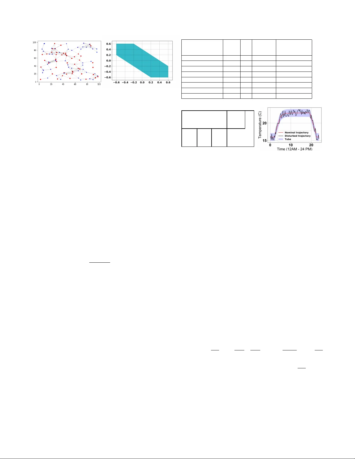
Compositional Synthesis of Decentralized Rob ust Set-In variance Contr ollers f or Large-scale Linear Systems Kasra Ghasemi, Sadra Sadraddini, and Calin Belta Abstract — Ensuring constraint satisfaction in large-scale sys- tems with hard constraints is vital in many safety critical sys- tems. The challenge is to design controllers that are efficiently synthesized offline, easily implementable online, and provide formal correctness guarantees. In this paper , we provide a method to compute correct-by-construction controllers for a network of coupled linear systems with additiv e bounded distur - bances such that i) the design of the controllers is fully composi- tional - we use an optimization-based appr oach that iteratively computes subsystem-level assume-guarantee contracts in the form of robust control inv ariant sets; and ii) the controllers are decentralized hence online implementation requires only the local state inf ormation. W e present illustrative examples, including a case study on a system with 1000 dimensions. I . I N T R O D U C T I O N Hard constraints on state and control exist in many sys- tems, where the controller should keep the state within a certain safe region using the admissible control inputs, no matter ho w the disturbances hit the system. Examples include collision av oidance in autonomous driving [1], capacity bounds in in ventory management [2], safety thresholds in anesthesia [3], and temperature bounds in heating, ventila- tion, and air conditioning (HV A C) systems [4]. It can be shown that the infinite-time constraint satisfaction problem is equiv alent to finding rob ust control in v ariant (RCI) sets [5], [6] in the state-space of the system. Existence of an RCI set guarantees existence of a control policy that keeps the state in the set for all times and for all allo wable disturbances. Giv en an RCI set, extracting the set-in variance controller is straightforward. RCI sets are commonly used to guarantee recursiv e feasibility in model predictiv e controllers (MPC) [6] (as the terminal constraint of the MPC opti- mization problem), or act as the set bounding the trajectory tracking error in tube MPC [7]–[12]. W e focus on two major shortcomings in computing and using RCI sets for large-scale systems. First, their computa- tion is e xpensiv e. Even though techniques for computing RCI sets for linear systems can be mapped to conv ex optimization problems [13], [14], the y are still computationally expensiv e for very lar ge problems [15]. Second, e ven when an RCI set is av ailable for a large-scale system, the controller is essen- tially centralized as it requires the global state kno wledge. This work was partially supported by the NSF under grants CPS- 1446151 and IIS-1723995 K. Ghasemi and C. Belta are with the Division of System Engineering, Boston Univ ersity , Boston, MA 02215, USA kasra0gh@bu.edu , cbelta@bu.edu S. Sadraddini is with the Computer Science and Artificial Intelli- gence Laboratory , Massachusetts Institute of T echnology , Cambridge, Mas- sachusetts 02139, USA sadra@mit.edu W e consider lar ge-scale linear systems with set-v alued ad- ditiv e disturbances and provide a fully compositional method to design decentralized set-inv ariance controllers. The nov- elty of the method lies in the fact that the coupling terms between subsystems are treated as set-valued disturbances, and the method iterati vely shrinks these coupling effects such that the obtained RCI sets are small, hence subsystems would operate closely to their nominal points or trajectories. The RCI sets are parameterized as zonotopes and act as assume- guarantee contracts between subsystems. W e use zonotope order reduction methods [16], [17] to limit the complexity growth of zonotopes o ver the iterations, which terminates when the obtained RCI sets conv erge. Related w ork The efficient computation of formally cor- rect controllers for large-scale systems is an acti ve area of research. Designing assume guarantee contracts for mono- tone dynamical systems was studied in [18], [19]. For safety specifications, assume guarantee contracts become closely related to RCI sets [20]. A close work to this paper is [21], where the authors formulated the problem of finding separable, decentralized RCI sets for linear systems with con- stant linear feedback gains using linear matrix inequalities (LMIs). While this method yields decentralized RCI sets and controllers, it is not compositional and the underlying LMI is solved for the whole system. W e applied our method to an example in [21] and compared the results. The authors in [22] formulated a similar problem and provided a solution similar to the one in this paper in the respect that they also treated the coupling terms as disturbances. Ho wev er , the ke y difference is that they considered coupling terms to be fixed - each subsystem was assumed to be able to take state and controls from the whole set of its admissible v alues. This assumption leads to very strong couplings and large RCI sets or ev en infeasibility . In reality , the coupling terms can be made smaller by restricting the state and controls of each subsystem to tak e v alues from smaller sets in their admissible sets. The question remains how to choose these sets in a “correct” and compositional way . This paper follows this line of idea as we iterati vely shrink the coupling effects to obtain smaller RCI sets. I I . N O T A T I O N A N D P R E L I M I NA R I E S The n -dimensional Euclidean space is denoted by R n . W e use N to denote the set of positive integers and define N q := { x ∈ N , x ≤ q } , q ∈ N . The Minkowski sum of two sets A ⊂ R n and B ⊂ R n is defined as A ⊕ B := { a + b | a ∈ A , b ∈ B } . The diagonal matrix obtained from the elements of a v ector h ∈ R n is denoted by diag( h ) ∈ R n × n . The m by n zero matrix is denoted by 0 m × n and identity matrix of size n is shown by I n . Giv en A ∈ R n × m , the 1-norm of matrix A is denoted by || A || 1 and is equal to P n i =1 P m j =1 | a ij | , where a ij is the element of matrix A in i th ro w and j th column. The element-wise absolute value of A is denoted by | A | . Giv en a set X ⊂ R n and A ∈ R m × n , we define A X := { Ax | x ∈ X } . Giv en two matrices A 1 , A 2 with the same number of rows, the matrix obtained from their horizontal concatenation is denoted by [ A 1 , A 2 ] . A zonotope Z ( c, H ) ⊂ R n is defined as: Z ( c, H ) := { c } ⊕ H B p , (1) where H ∈ R n × p . The columns of H are called generator s , c ∈ R n is its center , and B p := { x ∈ R p ||| x || ∞ ≤ 1 } . The zonotope order is defined as ( p n ) . The Minko wski sum of two zonotopes in R n can be written as: Z ( c 1 , H 1 ) ⊕ Z ( c 2 , H 2 ) = Z ( c 1 + c 2 , [ H 1 , H 2 ]) . (2) Consider a discrete-time linear system in the form: x ( t + 1) = Ax ( t ) + B u ( t ) + d ( t ) , (3) where x ∈ X , u ∈ U , and d ∈ D . The sets X, D ⊂ R n and U ⊂ R m define constraints for the state, disturbance, and control, respecti vely . The matrices A ∈ R n × n and B ∈ R n × m are constant and t ∈ N denotes the discrete time. Definition 1 (RCI set): An RCI set for system (3) is a set Ω ⊆ X for which there exists at least one controller that keeps the state of the system in that set for the next time step, for all allo wable disturbances: ∀ x ( t ) ∈ Ω , ∃ u ( t ) ∈ U, ∀ d ( t ) ∈ D ⇒ x ( t + 1) ∈ Ω . (4) I I I . P R O B L E M F O R M U L AT I O N In this section, we formalize the problem of set-in variance controller design for a network of dynamically coupled discrete-time linear systems that hav e the following form: x i ( t + 1) = A ii x i ( t ) + B ii u i ( t ) + X j 6 = i A ij x j ( t )+ X j 6 = i B ij u j ( t ) + d i ( t ) , (5) where x i ( t ) ∈ X i , X i ⊂ R n i , u i ( t ) ∈ U i , U i ⊂ R m i , and d i ( t ) ∈ D i , D i ⊂ R n i are the state, control input, and disturbance for subsystem i , respecti vely; A ii ∈ R n i × n i and B ii ∈ R n i × m i characterize the internal dynamics of subsystem i ; A ij ∈ R n i × n j and B ij ∈ R n i × m j characterize the coupling effects of subsystem j on subsystem i ; and i ∈ I , where I is the index set for subsystems. Pr oblem 1: Gi ven system (5), find sets Ω i and Θ i for all i ∈ I such that Ω i ⊆ X i , Θ i ⊆ U i , and ∀ x i ( t ) ∈ Ω i , ∃ u i ( t ) ∈ Θ i , ∀ x j ( t ) ∈ Ω j , ∀ u j ( t ) ∈ Θ j ( j 6 = i ) , ∀ d i ( t ) ∈ D i ⇒ x i ( t + 1) ∈ Ω i . (6) Throughout the paper , we assume that the matrix pairs ( A ii , B ii ) are controllable for all i ∈ I and the sets X i , U i , and D i are Z (0 , G x i ) , Z (0 , G u i ) , and Z (0 , G d i ) , respecti vely , where matrices G x i ∈ R n i × p x i , G u i ∈ R m i × p u i , and G d i ∈ R n i × p d i are given. Note that this assumption is not restricti ve in most common problems, since zonotopes are flexible objects that approximate most symmetric sets. Also, as it will become clear later in the paper, by under-approximating X i and U i and over -approximating D i , our solution to Problem 1 remains correct b ut becomes conserv ative. I V . S I N G L E R C I S E T C O M P U TA T I O N In this section, we provide a method to find an RCI set for a single system. The extracted controller is centralized and its implementation requires a con vex program - it can be shown that the controller can be explicitly represented as a piecewise affine function of the state, although we seldom find it useful to compute it. The follo wing method provides a bound on this extracted controller . The bound is named action set and is denoted by Θ . The RCI set computation method presented here is closely related to the one in [13]. Theor em 1: Let system (3) with constraints on the state and input control and D = Z (0 , G d ) , where G d ∈ R n × p . If ∃ k ∈ N , and matrices T ∈ R n × k and M ∈ R m × k such that the following relation holds: [ AT + B M , G d ] = [0 n × p , T ] (7) Z (0 , T ) ⊆ X (8) Z (0 , M ) ⊆ U, (9) then Ω = Z (0 , T ) is an RCI set. Pr oof: Note that the structure of matrices T and M is not unique and the value of k can be changed to deri ve different T and M . This enables iterations ov er different k . Substituting x = T b and u = M b where b ∈ B k in (3): x ( t + 1) = A ( T b ) + B ( M b ) + d ∈ ( AT + B M ) B k ⊕ G d B p = [ AT + B M , G d ] B ( k + p ) If Z (0 , T ) is an RCI set, x ( t + 1) should be in the set T B k and it can happen if the follo wing relation is satisfied: [ AT + B M , G d ] B ( k + p ) = T B ( k ) . (10) W e can augment the right hand side of (10) by adding p zero vector to the left of the matrix T to equate the dimensions of left hand matrices on both sides and reach: [ AT + B M , G d ] B ( k + p ) = [0 n × p , T ] B ( k + p ) . (11) If T and M satisfy the condition below , it implies that (11) is satisfied and Z (0 , T ) is the RCI set: [ AT + B M , G d ] = [0 n × p , T ] . (12) State and control input constraints force (8) and (9). Constraints (8) and (9) can be added, together with other constraints, to an optimization problem for the calculation of the RCI set. W e refer the readers to [23] where the authors presented a set of linear constraints for the zonotope containment problem. The objectiv e is to minimize || T || 1 , means minimizing all the elements of matrix T . It is a suitable linear heuristic to make the volume of RCI set Z (0 , T ) small. Other heuristics may also be employed. Thus, we find the RCI set by the following linear program (LP): argmin T ,M || T || 1 subject to [ AT + B M , G d ] = [0 n × p , T ] Z (0 , M ) ⊆ Z (0 , G u ) Z (0 , T ) ⊆ Z (0 , G x ) . (13) The final algorithm to find the RCI set ( Ω ) and the action set ( Θ = Z (0 , M ) ) is sho wn in Algorithm 1. Algorithm 1 Single RCI Require: A, B , G x , G u , G d 1: Initializing: k = 1 2: while False infeasibility do 3: T , M ← Solving Optimization Problem (13) 4: k ← k + 1 5: end whilereturn T , M Remark 1: Both methods in Theorem 1 and [13] are able to deriv e the same RCI sets albeit they are different in formulations and the choice of variables. First, the authors in [13], considered the matrices T ∈ R n × pk and M ∈ R m × pk in the form of [ T 1 , · · · , T k ] and [ M 1 , · · · , M k ] , where each T q ∈ R n × p and M q ∈ R m × p ( q ∈ N k ) , respectively . This implies that the number of columns in T is a multiplication of p , whereas this is not necessarily the case in our formulation. Second, the RCI set in [13] is in the form of Mink owski sum of mapped disturbance sets, L k q =1 T q D . V . I T E R A T I V E C O M P O S I T I O NA L R C I S E T S Y N T H E S I S Now , we present the main contribution of this paper . The main idea is to treat state and control couplings acting on a subsystem as disturbances. It is irrational to characterize such disturbance as caused by the whole admissible set of the states and controls of other subsystems. Instead, the other subsystems only operate in a limited set of states and using a limited set of control inputs. So, couplings are smaller and essentially depend on the whole system behavior . Achieving it needs a circular method and we start this circularity by initializing by some arbitrary sets of admissible states and controls and shrinking these sets using an iterativ e measure. A natural candidate for initial sets are (scalar multiplications of) the whole set of admissible values. The obtained RCI sets and its corresponding set of control inputs are then used as new constraints and couplings, which can be used to reiterate the computation of RCI sets. This procedure continues and all of the RCI sets will be recomputed for each subsystem individually . The resulting RCI sets and their corresponding admissible control sets shrink by construction. Thus, the successiv e iterations lead to con vergence. This method is effecti vely constructing assume-guarantee contracts in the form of RCI sets, where we declare assumptions on states and control inputs of coupled subsystems j and in return guarantee that the state and the control input of the subsystem i remain inside certain sets. A. State and Contr ol Input Coupling as Disturbance In order to address the aforementioned problem in a com- positional manner where each subsystem is solv ed indepen- dently , the couplings between the subsystems are re garded as disturbances. W e initiate the method with x i ∈ Z (0 , G x i ) and u i ∈ Z (0 , G u i ) for all i . Therefore, for subsystem i the disturbance set can be seen as: M j 6 = i A ij Z (0 , G x j ) ⊕ M j 6 = i B ij Z (0 , G u j ) ⊕ Z (0 , G d i ) . (14) Since zonotopes are closed under Minko wski sum, we can rewrite the abo ve expression as: Z (0 , [ A i 1 G x 1 , · · · , A ij G x j , B i 1 G u 1 , · · · , B ij G u j , G d i ] | {z } G extend i ) , (15) which brings the system in (5) to the follo wing form: x i ( t + 1) = A ii x i ( t ) + B ii u i ( t ) + d extend i , (16) where d extend i ∈ Z (0 , G extend i ) . By using Algorithm 1, the RCI set and action set can be computed. In order to hav e shrinking RCI sets, the last tw o constraints in (13) are modified to reflect the new bounds for the state and control inputs, so that the ne w RCI and action sets become subsets of the ones in the last iteration. B. Zonotope Order Reduction Zonotope order reduction methods help us to over - approximate a zonotope Z ( c, H ) by a zonotope with fe wer generators (smaller order). This technique is useful in recur- siv e methods that increase zonotope order, as operations with high order zonotopes are computationally expensiv e. There are several methods for zonotope order reduction [16], [17]. Boxing method [24], [25] over -approximates the zonotope by a box that has the following upper and lo wer bounds: c − p X i =1 | h i | ≤ Z ( c, H ) ≤ c + p X i =1 | h i | , (17) where H ∈ R n × p and h i is its generator . These bounds correspond to a box that is represented by reduce ( H ) . W e dropped c , because it is always zero in our case. So, reduce ( H ) := diag( X i | h i | ) . (18) Since the order of disturbance in (16) is large and gets ev en larger with the number of iterations, we use the zonotope order reduction method to improve computational complexity . So, the disturbance set can be replaced by Z (0 , reduce ( G extend i )) . Note that zonotope order reduction methods gi ve an over -approximation of the input zonotope, therefore, a tighter over -approximation of the disturbance set results in a less conservati ve solution. In this paper , we used the boxing method for zonotope order reduction. The iterativ e procedure is shown in Algorithm 2. Algorithm 2 Compositional decentralized RCI Algorithm Require: A ii , A ij , B ii , B ij , G x i , G u i , G d i , ∀ i, j ∈ I 1: Initializing: T i ← G x i , M i ← G u i 2: while all T i and all M i Con vergence do 3: for i ∈ I do 4: G extend i ← (15) 5: G new i ← reduce( G extend i ) 6: T i , M i ← Single RCI ( A ii , B ii , T i , M i , G new i ) 7: end for 8: end whilereturn Z (0 , T i ) , Z (0 , M i ) , ∀ i ∈ I C. Computational Complexity For polynomial-time interior -point LP solvers, the worst case complexity is O ( β 3 . 5 ) , where β is the number of vari- ables and constraints [26]. Considering system (5) and using the boxing method, the number of v ariables and constraints for each single LP in Algorithm 2 is: O ([ n 2 i + n i + m i + (10 n i + 6 m i ) k i ] 3 . 5 ) , (19) where k i is the number of columns in the RCI generator , typically observ ed to be at the same order of the contollabil- ity index of ( A ii , B ii ) . The total number of LPs to be solved is |I | times the number of iterations in Algorithm 2. V I . C A S E S T U D I E S In this section, we consider three case studies. In the first case, we compare our method to [21]. In the second one, we demonstrate the scalabilty of our approach on a large system. Finally , we utilize our method to control an HV A C system to show its applicability in engineering problems. (a) subsystem 1 (b) subsystem 2 (c) subsystem 3 Fig. 1: The RCI sets obtained for each subsystem in case study 1 using our approach. Fig. 2: The RCI sets presented in [21]. Subsystems 1 to 3 are shown from left to right. The RCI sets are in red (the blue areas are the possible states in the next time step). A comparison with Fig. 1 sho ws that our approach results in smaller RCI sets. A. Case study 1 This example is adopted from [21], where the authors considered the following dynamics for each subsystem: x + i = α i R ( θ ) x i ( t ) + u i ( t ) + X i 6 = j β ij x j + d i ( t ) , (20) where R ( θ ) is the counter -clockwise rotation matrix in R 2 , x i ( t ) , u i ( t ) , d i ( t ) ∈ R 2 are the state, control input, and disturbance. The control input and disturbance are bounded: || u i || ∞ ≤ 0 . 65 and || d i || ∞ ≤ 0 . 4 . Similar to [21], we consider three subsystems. W e use α i = 0 . 8 and β ij can take two v alues: 0 . 1 if | i − j | = 1 and 0 otherwise. The results of our method are illustrated in Fig. 1, while the results of [21] are sho wn in Fig. 2. The adv antages of our method against [21] are as follows: i) we obtain smaller RCI sets, ii) it is faster since it is compositional, and iii) it does not assume any specific shape for the input controllers - in [21], the authors assume the controllers to be linear . They reported 11 seconds of computation time whereas our method took 0.25 second on a MacBook Pro 2.6 GHz Intel Core i7. B. Case study 2 Here we test our approach on a large scale system. Inspired by [27], we generate a random lar ge system. In [27], the authors initially scatter random points in a square field and (a) (b) Fig. 3: Case study 2: (a) an e xample of a random system. The threshold is 15 and if tw o points are connected with an edge, they are neighbors. (b) An RCI set for one of the subsystems when the state dimension in the aggregated system is 100, λ = 100 , and R = 10 . assign each potint to a subsystem. If the Euclidean distance between any two points is less than a user-defined threshold ( R ), they are considered as neighbors. In order to generate more asymmetry , we distribute two classes of subsystems where each class has its o wn A ii . As illustrated in Fig. 3a, we distribute equal numbers of red and blue subsystems in the field. The dynamics for each subsystem is: x + i = A ii x i ( t ) + B ii u i ( t ) + d i ( t ) + X j 6 = i A ij x j ( t ) , (21) where A ii s are  1 1 1 2  and  1 1 0 1  for red and blue sub- systems, respectiv ely . F or all subsystems, B ii is  0 1  . If subsystems i and j are not neighbors, A ij = 0 . Otherwise: A ij = λ dist( i, j )  1 0 0 1  , (22) where λ is a constant and dist( i, j ) is Euclidean distance between points i and j in Fig. 3a. The following constraints are imposed on (21): x i ( t ) ∈ Z (0 , 10 I 2 ) , u i ( t ) ∈ Z (0 , 10 I 1 ) , d i ( t ) ∈ Z (0 , 0 . 2 I 2 ) . (23) The ex ecution time for finding RCI sets in different condi- tions are reported in T able I. Since the size of the field is fixed, as the number of subsystems increase, the couplings get stronger . For v ery large couplings, the disturbance be- comes v ery large such that it leads to infeasiblity in LPs. Thus, we alter λ and R to adjust the disturbances to maintain feasibility . Finally , as a sample, one of the RCI sets is illustrated in Fig. 3b. T ABLE I: Case study 2 State dimension of aggregated system λ R Number of iterations T otal execution time (Seconds) 100 0.01 1 3 0.36 100 0.01 10 3 0.95 100 0.001 1 3 0.36 100 0.001 10 3 0.95 1000 0.01 1 5 6.64 1000 0.01 10 5 225 1000 0.001 1 3 3.93 1000 0.001 10 3 137.22 room 6 Hallway room 5 Conference room room 1 Carpentry room room 2 Casting room room 3 Robotics Lab (a) room 4 Offices (b) Fig. 4: Case study 3: (a) The plan of EPIC building at Boston Univ ersity . (b) nominal trajectory , tube, and disturbed trajectory for subsystem (room) 6. The disturbed trajectory remains inside the tube for all time. The other subsystems hav e similar trajectories. C. Case study 3 As the third example, we consider the control of a HV AC system. W e require that the temperature in a building follows a desired trajectory so that we can sa ve energy during of f- hours and also maintain the desired temperature in office hours. W e model the HV A C system in the EPIC b uilding at Boston university . There are 6 separate spaces on the ground floor . The floor plan is shown in Fig. 4a . W e borrow the model from [28] and [29], which is the follo wing: T + i = A ii T i ( t ) + X j ∈N i A ij T j ( t ) + B i u i ( t ) + E i d i ( t ) , (24) where T i , the state of subsystem i is the temperature of room i , and u i , the control input is the rate of ener gy HV A C system releases in its surroundings; d i is the disturbance that can be the result of transferring heat to the outside en vironment, human bodies, or other unkno wn factors; N i is a set of rooms neighbouring room i . The matrices are: A ii = 1 − ∆ τ c i ( X j ∈N i 1 R i,j + 1 R o,i ) , A ij = ∆ τ R i,j c i , B i = ∆ τ c i , E i = ∆ τ c i , (25) where ∆ τ is the time step assumed to be 15 minutes. c i = 1 . 375 × 10 3 K J K is the thermal capacitance of the air in room i . R i,j = 14 K W K and R o,i = 50 K W K are the thermal resistance between room i and j and the thermal resistance between room i and the outside environment, respectively . The bounds on each u i ( t ) and d i ( t ) are: 0 ≤ u i ( t ) ≤ 9 , − 1 . 6 ≤ d i ( t ) ≤ 1 . 6 . (26) W e use tube MPC [11],[12], which takes advantage of the superposition principle of linear systems and di vides the system into two. One is nominal, which tracks the trajectory , while the other one keeps the state of the system inside a tube around the nominal trajectory . The cross section of the tube at each time step is the RCI set. The results for room 6 are shown in Fig. 4b . V I I . C O N C L U S I O N S A N D F U T U R E W O R K W e presented a compositional method to derive minimal approximation of decentralized rob ust control in variant sets for discrete-time linear time-in v ariant systems. Our approach uses iterative linear programs, which makes it very fast and applicable to large systems by breaking them into subsystems. Our method does not rely on linear controllers and it is correct-by-construction. In future work, we will in vestigate using different meth- ods for zonotope or der reduction to get tighter ov er- approximation of disturbances hence reducing conservatism. In addition, we will consider extending our method to deal with nonlinear and hybrid dynamics, with a particular focus on piecewise affine models. R E F E R E N C E S [1] A. Al Alam, A. Gattami, and K. H. Johansson, “ An experimental study on the fuel reduction potential of heavy duty vehicle platooning, ” in 13th International IEEE Conference on Intelligent T ransportation Systems . IEEE, 2010, pp. 306–311. [2] F . Borrelli, C. Del V ecchio, and A. Parisio, “Robust inv ariant sets for constrained storage systems, ” A utomatica , 2009. [3] M. Y ousefi, K. v an Heusden, N. W est, I. M. Mitchell, J. M. Ansermino, and G. A. Dumont, “ A formalized safety system for closed-loop anesthesia with pharmacokinetic and pharmacodynamic constraints, ” Contr ol Engineering Practice , v ol. 84, pp. 23–31, 2019. [4] A. Afram and F . Janabi-Sharifi, “Theory and applications of hvac control systems–a revie w of model predictiv e control (mpc), ” Building and Envir onment , vol. 72, pp. 343–355, 2014. [5] F . Blanchini, “Set in variance in control The paper provides a surve y of the literature on in variant sets and their applications, ” T ech. Rep., 1999. [6] E. C. Kerrig an, “Robust constraint satisfaction: Inv ariant sets and predictiv e control, ” Ph.D. dissertation, University of Cambridge, 2001. [7] S. V . Rakovic and D. Q. Mayne, “Set Robust Control Inv ariance for Linear Discrete T ime Systems, ” T ech. Rep. [8] D. Q. Mayne, E. C. K errigan, E. V an W yk, and P . Falugi, “T ube-based robust nonlinear model predicti ve control, ” International Journal of Robust and Nonlinear Contr ol , vol. 21, no. 11, pp. 1341–1353, 2011. [9] S. Y u, C. Maier , H. Chen, and F . Allg ¨ ower , “Tube mpc scheme based on rob ust control inv ariant set with application to lipschitz nonlinear systems, ” Systems & Control Letter s , vol. 62, no. 2, pp. 194–200, 2013. [10] J. B. Rawlings and D. Q. Mayne, Model pr edictive contr ol: Theory and design . Nob Hill Pub . Madison, W isconsin, 2009. [11] S. V . Rakovic and D. Q. Mayne, “ A simple tube controller for efficient robust model predictive control of constrained linear discrete time systems subject to bounded disturbances , ” T ech. Rep. [12] D. Q. Mayne, “Model predicti ve control: Recent developments and future promise, ” 2014. [13] S. V . Rak ovic, E. C. Kerrigan, D. Q. Mayne, and K. I. K ouramas, “Optimized robust control inv ariance for linear discrete-time systems: Theoretical foundations, ” Automatica , vol. 43, no. 5, pp. 831–841, 2007. [14] S. V . Rako vic and M. Baric, “Parameterized rob ust control in variant sets for linear systems: Theoretical advances and computational re- marks, ” IEEE T ransactions on A utomatic Contr ol , v ol. 55, no. 7, pp. 1599–1614, 2010. [15] S. Sadraddini, S. Sivaranjani, V . Gupta, and C. Belta, “Prov ably safe cruise control of vehicular platoons, ” IEEE Control Systems Letters , vol. 1, no. 2, pp. 262–267, 2017. [16] A. K. K opetzki, B. Schurmann, and M. Althoff, “Methods for order reduction of zonotopes, ” 2017 IEEE 56th Annual Conference on Decision and Contr ol, CDC 2017 , vol. 2018-Janua, no. Cdc, pp. 5626– 5633, 2018. [17] X. Y ang and J. K. Scott, “A comparison of zonotope order reduction techniques, ” Automatica , 2018. [18] E. S. Kim, M. Arcak, and S. A. Seshia, “Compositional controller syn- thesis for vehicular traf fic networks, ” in 2015 54th IEEE Conference on Decision and Contr ol (CDC) . IEEE, 2015, pp. 6165–6171. [19] ——, “Directed specifications and assumption mining for monotone dynamical systems, ” in Proceedings of the 19th International Confer- ence on Hybrid Systems: Computation and Contr ol . A CM, 2016, pp. 21–30. [20] S. Sadraddini, J. Rudan, and C. Belta, “Formal synthesis of distributed optimal traffic control policies, ” in 2017 ACM/IEEE 8th International Confer ence on Cyber-Physical Systems (ICCPS) . IEEE, 2017, pp. 15–24. [21] P . Nilsson and N. Ozay , “Synthesis of separable controlled in variant sets for modular local control design, ” Proceedings of the American Contr ol Conference , vol. 2016-July , pp. 5656–5663, 2016. [22] S. Scialanga and K. Ampountolas, “Rob ust constrained interpolating control of interconnected systems, ” in 2018 IEEE Confer ence on Decision and Contr ol (CDC) . IEEE, 2018, pp. 7016–7021. [23] S. Sadraddini and R. T edrake, “Linear encodings for polytope con- tainment problems, ” arXiv preprint , 2019. [24] W . Kiihn, “Rigorously Computed Orbits of Dynamical Systems with- out the Wrapping Effect, ” T ech. Rep., 1998. [25] C. Combastel, “ A state bounding observer based on zonotopes. in proc. of the european control conference, ” p. 25892594, 2003. [26] N. Karmarkar, “A˜New Polynomial-T ime Algorithm for Linear Pro- gramming, ” T ech. Rep., 1984. [27] N. Motee and A. Jadbabaie, “Optimal Control of Spatially Distributed Systems, ” vol. 53, no. 7, pp. 1616–1629, 2008. [28] Y . Long, S. Liu, L. Xie, and K. H. Johansson, “A hierarchical distributed MPC for HV A C systems, ” Proceedings of the American Contr ol Conference , vol. 2016-July , pp. 2385–2390, 2016. [29] Z. W ang, G. Hu, and C. J. Spanos, “Distributed model predictiv e control of bilinear HV A C systems using a con vexification method, ” 2017 Asian Contr ol Confer ence, ASCC 2017 , vol. 2018-Janua, no. 3, pp. 1608–1613, 2018.