Shapley Interpretation and Activation in Neural Networks

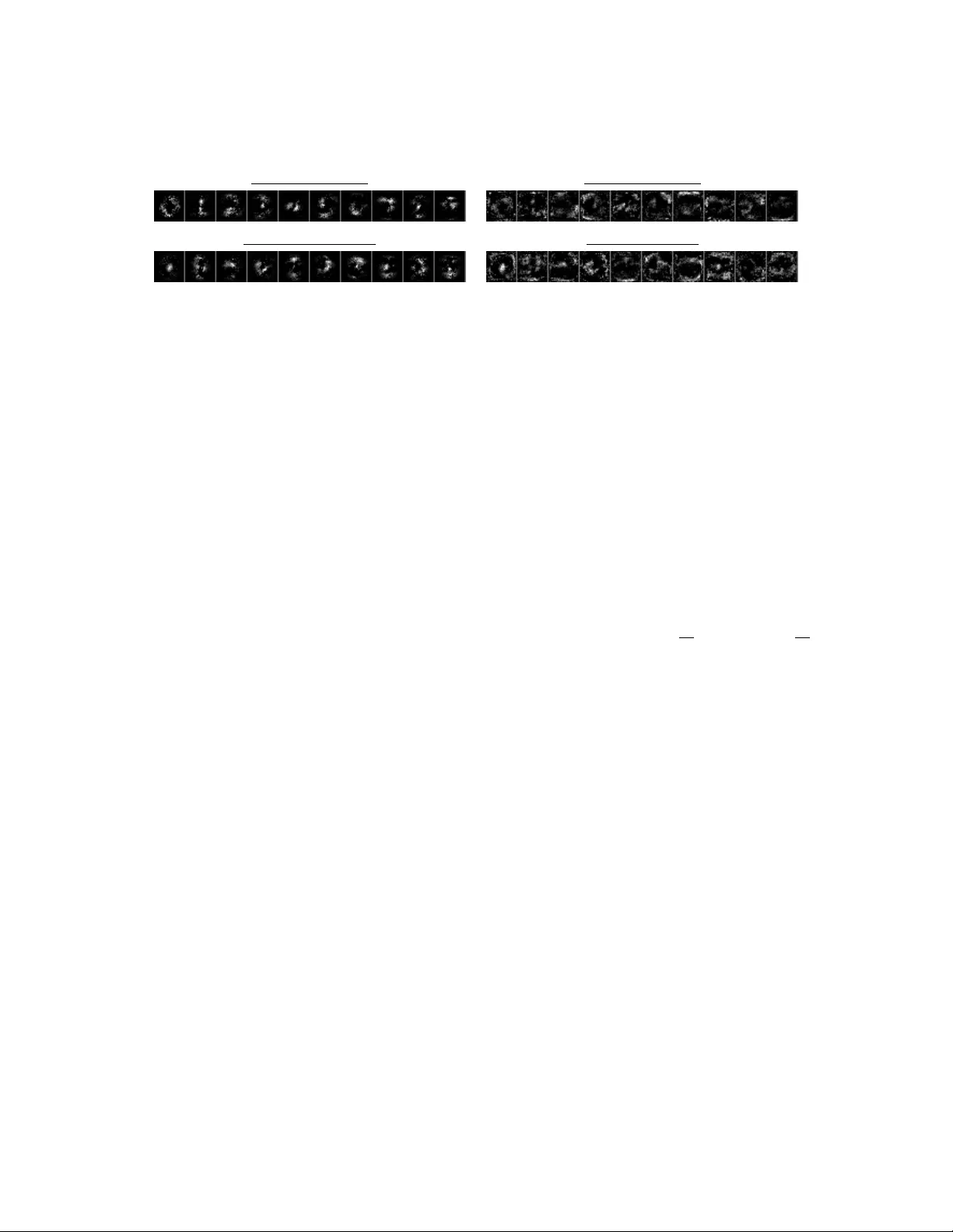
Shapley Interpret a tion and A ctiv a tion in Neural Netw orks Y adong Li and Xin Cui ∗ Septem b er 18, 2019 Abstract W e prop ose a nov el Shapley v alue approach to help address neural net works’ in terpretability and “v anishing gradien t” problems. Our method is based on an accurate analytical appro ximation to the Shapley v alue of a neuron with ReLU activ ation. This analytical appro ximation admits a linear propagation of relev ance across neural netw ork lay ers, resulting in a simple, fast and sensible in terpretation of neural net works’ decision making pro cess. W e then deriv ed a globally con tinuous and non-v anishing Shapley gradient, which can replace the con ven tional gradient in training neural netw ork la yers with ReLU activ ation, and leading to b etter training p erformance. W e further deriv ed a Shapley Activ ation (SA) function, whic h is a close approximation to ReLU but features the Shapley gradient. The SA is easy to implement in existing mac hine learning framew orks. Numerical tests show that SA consistently outp erforms ReLU in training conv ergence, accuracy and stability . 1 In tro duction Deep neural netw ork has achiev ed phenomenal success during the past decade. How ever, many challenges remain, among which interpretabilit y and the “v anishing gradient” are tw o of the most w ell-known and critical problems [1, 2]. It is difficult to interpret how a neural netw ork arrives at its output, esp ecially for deep netw orks with man y lay ers and an enormous n umber of parameters. Often times, users view a neural netw ork as a “black b o x” that magically works. Lack of interpretabilit y is often one of the top concerns [ 3 – 12 ] among users who ha ve to make real world decisions based on neural netw orks’ outputs. When a neural netw ork grows deep and large, many of its neurons inevitably b ecome dormant and stopp ed con tributing to the final output, causing the problem of “v anishing gradien t”. As a result, individual training data ma y only up date a small fraction of the neurons, th us prolonging the training pro cess. The v anishing gradien t may also cause an optimizer to stop prematurely . Therefore, large neural net works usually require m ultiple rep etitions of training runs, to increase the c hance of con verging to a go od solution. There are several p opular tec hniques for mitigating the problem of v anishing gradient [ 13 – 21 ]. One of them is the ReLU activ ation function [ 22 ] and its v ariants, such as leaky ReLU [ 23 ], noisy ReLU [ 24 ] and SeLU [ 25 ]. The ReLU family of activ ation functions are known for preserving gradients b etter o ver deep net works than other t yp es of activ ation functions. Preserving gradien t is also the flagship features in man y p opular neural netw ork architectures, such as ResNet [ 26 ]. Batch normalization [ 27 ] is a recent breakthrough that is prov en effectiv e for preserving gradient in deep netw orks. Despite these mitigations, the v anishing gradien t remains a c hallenge and con tinues to impose a practical limit on the size of a neural netw ork, b ey ond whic h the training becomes infeasible. In this pap er, we prop ose a Shapley v alue [ 28 ] approach for b etter interpreting a neural netw orks’ prediction and improving its training by preserving gradient. Shapley v alue is a well established metho d in the co operative game theory , and it forms a solid theoretical foundation to analyze and address b oth ∗ Barclays, the views express in this article is the authors’ own, they do not necessarily represen t the views of Barclays. W e thank Mohammad Jahangiri, Antonio Martini and Ariye Shater for man y helpful comments and discussions, whic h made this paper significantly b etter. All remaining errors are authors’ o wn. 1 T able 1: Shapley V alue Example with Three Inputs and ReLU Activ ation P ermutation s = P i ∈ S w i x i + b max( s, 0) Incremen tal Contribution ~ w = (1 , 2 , 3) , b = − 1 x 1 = -1 x 2 = 2 x 3 = -1 x 1 , x 2 , x 3 -2, 2, -1 0, 2, 0 0 2 -2 x 1 , x 3 , x 2 -2, -5, -1 0, 0, 0 0 0 0 x 2 , x 1 , x 3 3, 2, -1 3, 2, 0 -1 3 -2 x 2 , x 3 , x 1 3, 0, -1 3, 0, 0 0 3 -3 x 3 , x 1 , x 2 -4, -5, -1 0, 0, 0 0 0 0 x 3 , x 2 , x 1 -4, 0, -1 0, 0, 0 0 0 0 Av erage α 1 = − 1 6 α 2 = 4 3 α 3 = − 7 6 problems. Due to the great success and ubiquity of the ReLU activ ation function, we focus our efforts in finding a solution that can be viewed as a v ariant or appro ximation to the ReLU activ ation. 2 Metho dology In a typical neural net work, a neuron with n inputs can b e written as: y = f ( P n i =1 w i x i + b ), where f ( · ) is a nonlinear activ ation function, ~ x are the input to the neuron and ~ w , b are the internal parameters of the neuron. 2.1 Shapley V alue In terpretation Shapley v alue w as originally dev elop ed for fairly distributing shared gain or loss of a team among its team mem b ers. It has since b een widely used in many different fields, suc h as the allo cation of shared sale pro ceeds of pac k age deals among participating service pro viders. If w e are interested in the con tribution (a.k.a. relev ance) of a giv en input x k to the output y of a neuron, Shapley v alue is the only correct answer in theory [ 28 ]. Shapley v alue of an input x k is defined to b e the a verage of its incremen tal contributions to the output y o ver all p ossible p erm utations of x i s. W e use α k to denote the Shapley v alue of a neuron’s input x k , and Shapley v alue is conserv ativ e by construction: y = P n i =1 α i . T able 1 is an example of computing Shapley v alue of a neuron with 3 inputs. The column “ s = P n i =1 ( w i x i + b )” and “ max ( s, 0)” are the inputs and outputs of the ReLU when one, t wo or three inputs are activ ated in the order sp ecified in the column “P ermutation”. In this example, there are 6 p ossible p erm utations for 3 inputs, th us the Shapley v alue for any of the inputs is the av erage of its incremen tal con tributions ov er all six possible p erm utations. It is imp ortan t to observe that the Shapley v alue of all 3 inputs are nonzero, even though the ReLU is curren tly deactiv ated with an ov erall output of 0. The reason for non-zero Shapley v alues is that the neuron could b e activ ated by tw o combinations of inputs ( x 2 ) or ( x 1 , x 2 ) in this example. There is some similarity b et ween the computation of Shapley v alue and the random drop out neural net work [ 29 ], in the sense that a random p ortion of the inputs are remo ved. How ever, it is worth p oin ting out their difference: a random drop out neural net work turns off inputs randomly with an indep enden t probabilit y p , whic h leads to muc h higher c hance of ha ving roughly (1 − p ) n activ e inputs. In con trast, random permutation works in tw o steps: first a single uniform random in teger ˜ h b et w een 0 and n is dra wn; then a random ordering of the n inputs is draw and only the first ˜ h inputs in the permutation are kept on. Random permutation therefore gives equal probability in activ ating any num b er of inputs betw een 0 and n , yielding better chance of activ ating the neuron than random drop outs. F or a generic activ ation function f ( · ), Shapley v alue can only b e ev aluated n umerically , for example using Mon te Carlo sim ulation. Suc h a n umerical implementation is computationally exp ensiv e and not conduciv e 2 to analysis. Recen tly , an accurate analytical appro ximation to the Shapley v alue of the gain/loss function in the form of max ( P i a i , P i b i ) was discov ered and v erified in [ 30 ], the same approac h can be adapted to ReLU activ ation function of y = max( P n i =1 w i x i + b, 0), resulting in an analytical appro ximation of: µ = 1 2 n X i =1 w i x i σ 2 = 1 6 n X i =1 ( w i x i ) 2 + 1 12 n X i =1 w i x i ! 2 (1) α k ≈ Φ( µ + b σ )  w k x k + b n  where Φ( · ) is the standard normal distribution function, and α k is the Shapley v alue of the k-th input. The relev ance of a neuron’s output y is defined to b e its contribution to the final output of the en tire neural net work, which is t ypically a prediction or probability (e.g. in classification problems). If w e denote relev ance of a neuron’s output as r ( y ), a simple method to propagate the relev ance to the neuron’s inputs x k is to tak e adv antage of the linearity of Shapley v alue and multiply a factor r ( y ) y to both side of y = P n i =1 α i ; and w e arriv e at the follo wing propagation form ula after some rearrangement: r ( x k ← y ) = α k P n i =1 α i r ( y ) ≈ w k x k + b n P n i =1 w i x i + b r ( y ) (2) where r ( x k ← y ) is the relev ance propagation from the neuron’s output y to input x k . T otal relev ance is conserv ed b et ween lay ers as r ( x k ) is the sum of r ( x k ← y ) from all the connected neurons in the follo wing la yer. Since the Φ( · ) factor cancels, the lay er-wise relev ance propagation (LRP) [31, 32] form ula is iden tical for linear and linear + ReLU la yers. If r ( y ) is initialized to b e the Shapley v alue of the neuron’s output y , then the r ( x k ) retains the interpretation of b eing the (approximated) Shapley v alue of neuron’s input x k after applying the LRP in (2) . A  · sign ( P n i =1 α i ) term with a small  > 0 can be added to the denominator of (2) to preven t it from v anishing, similar to the  -v ariant formula of [31, 32]. The output lay er of a neural net work is often a nonlinear function, such as the softmax for classification. Before w e can start the LRP via (2) , the relev ance of the output lay er has to be initialized to its Shapley v alue, whic h requires numerical ev aluation (such as Mon te Carlo) for most output functions, with few notable exceptions such as Linear and Linear+ReLU output la yers. The Shapley v alue of a Linear+ReLU output la yer is given by (1). An implicit assumption b ehind the LRP formula (2) is that the neuron’s activ ation are indep enden t from eac h other 1 , whic h generally does not hold across neural netw ork la yers. Therefore the Shapley v alues computed from LRP (2) is only a crude approximation for deep neural net works. A Monte Carlo simulation is required to compute the exact Shapley v alues of a neural netw ork’s input. Ho wev er, the LRP (2) has the adv antages of b eing v ery fast and producing the (appro ximated) relev ance of all hidden lay ers as w ell as the input lay er in one shot; while a MC approac h would require a separate sim ulation for eac h neural net work la yer. In practice, a crude appro ximation like (2) ma y often b e go od enough to give users the in tuition and confidence in using neural net work’s output. The LRP form ula (2) is similar to the native LRP algorithms giv en in [ 31 , 32 ], but it replaces w k x k b y ( w k x k + b n ). The b enefit of such a replacemen t is rather in tuitive by considering the limiting case of b  w i x i for all i , in which case individual w i x i no longer makes m uch difference to the output, thus all inputs’ relev ance propagation should b e appro ximately equal. By including the b n , (2) pro duces more sensible results for this limiting case than the known LRP form ulae in the literature. The approximation (1) offers a straigh t forw ard explanation on why the same propagation formula applies to b oth Linear and Linear+ReLU lay ers, which is a common feature in existing LRP algorithms. More generic appro ximations to Shapley v alues ha ve been developed in [ 8 , 33 ] for interpreting neural netw orks, in comparison the analytical approximation in (1) is faster and more con venien t for the ReLU la yers. 1 An example of the effect of correlation is to consider tw o lay ered neurons that can never activ ate together, then there should be no relev ance propagation through them, but formula (2) do es. 3 2.2 Shapley Gradien t As shown in T able 1, Shapley v alues are non-zeros for a neuron with ReLU as long as at least one of the input com binations can activ ate the neuron, it is muc h more lik ely than the neuron b eing active, which requires a m uch stronger condition of s = P n i =1 ( w i x i + b ) > 0. This observ ation motiv ated the follo wing approac h to prev ent the neuron’s gradients from v anishing: we use ∂ α k ∂ x k to replace the true gradient of ∂ y ∂ x k during the bac k propagation stage of the training. The result of this replacemen t is similar to a training pro cedure using random p erm utations, as men tioned earlier, random p erm utation is quite different from t ypical random drop outs. In mathematical terms, this alternativ e gradient is an appro ximation of: ∂ y ∂ ~ x = ∂ y ∂ ~ α ∂ ~ α ∂ ~ x ≈ ∂ y ∂ ~ α  ∂ ~ α ∂ ~ x ◦ I  =  ∂ α i ∂ x i  (3) ∂ ~ α ∂ ~ x is the full Jacobian matrix and ∂ ~ α ∂ ~ x ◦ I is a matrix with only the diagonal elements of ∂ ~ α ∂ ~ x , the ◦ is elemen t wise matrix pro duct. The last step is b ecause y = P n i =1 α i b y construction, th us ∂ y ∂ ~ α is a vector of 1s. Similar appro ximations are also applied to ~ w and b for back propagation: ∂ y ∂ x k ≈ ∂ α k ∂ x k = Φ( µ + b σ ) w k + g k w k  1 2 σ − ( µ + b )( w k x k + µ ) 6 σ 3  ∂ y ∂ w k ≈ ∂ α k ∂ w k = Φ( µ + b σ ) x k + g k x k  1 2 σ − ( µ + b )( w k x k + µ ) 6 σ 3  (4) ∂ y ∂ b ≈ n X k =1 ∂ α i ∂ b = Φ( µ + b σ ) + 1 σ n X k =1 g k where g k = φ ( µ + b σ )  w k x k + b n  , and φ ( · ) is standard normal distribution density function. The last terms of the first tw o equations in (4) are the contribution to the gradient from the Φ( µ + b σ ) factor, which is usually small in most practical situations and th us can b e safely ignored. W e subsequently refer to (4) as the Shapley gradien ts. The training process using Shapley gradients is similar to that of t ypical neural net works, except that (4) are used during bac k propagation stage for an y la yers with ReLU activ ation; the feed forw ard calculation of the neural netw ork remains unc hanged with the ReLU activ ation. W e subsequen tly use the term “Shapley Linear Unit” (ShapLU) to refer to the training scheme of mixing Shapley gradien t in the bac kward propagation with ReLU activ ation in the feed forward stage. Ev en though Shapley gradient is inconsisten t with the ReLU forward function, it is arguably a better c hoice for training neural net works; as it is more robust to descent to wards the av erage direction of the steep est descent of all possible p erm utations of a neuron’s inputs. The main adv antage of Shapley gradient is that it is globally con tinuous and nev er v anishes. Even when a neuron is deep in the off state with s = P n i =1 w i x i  0, significan t gradient could still flo w through when σ in (1) is large. F or example, when a single w i x i signal b ecome very strong in either p ositiv e or negative direction, the resulting increase in σ w ould open the gradient flow. This is a very nice prop ert y as it is exactly the righ t time to up date a neuron’s parameters when an y input signal is wa y out of line comparing to its p eers. W e call this property “attention to exception”. Figure 1 is a numerical illustration of this prop ert y , where we v ary one w k x k signal to a neuron and keep other inputs unchanged. The vertical axis is the Φ( µ + b σ ) factor, whic h con trols the rate of gradient flow from the output to the input of a neuron in (1). 2.3 Shapley Activ ation It requires some additional efforts to implement ShapLU in most mac hine learning framew orks, because a customized gradien t function has to b e used instead of automatic differentiation. T o ease the implementation of Shapley gradient, we set out to construct an activ ation function whose gradien t matc hes the Shapley gradien t, but main tains full consistency betw een the forw ard calculation and bac kward gradien t. The downside of suc h an activ ation function is that it can only b e an approximation to ReLU in the forward calculation. 4 Figure 1: Atten tion to Exceptions Figure 2: Shapley Activ ation (SA) Observ e that in (1) , the cross dep endency b et ween α i on x j , w j when i 6 = j is only through the factor Φ  µ + b σ  , whic h is a v ery smo oth function. The cross sensitivities ∂ α i ∂ x j are usually small in practical settings th us can be safely ignored. Therefore, w e can construct an (implied) activ ation function as the sum of all Shapley v alue α i s in (1), which is a close approximation to ReLU: max n X i =1 w i x i + b, 0 ! ≈ Φ  µ + b σ  n X i =1 w i x i + b ! (5) Giv en the cross sensitivities are usually small, the gradient of (5) closely matc hes the Shapley gradient in (4) . W e subsequently call (5) the Shapley Activ ation (SA), which is m uch easier to implement in existing machine learning framew orks via automatic differentiation. Unlik e typical activ ation functions that only dep ends on the aggregation of s = P n i =1 w i x i + b , the activ ation function defined in (5) dep ends on ~ x, b, ~ w , thus having a muc h more sophisticated activ ation profile. T ypical activ ation functions can b e plotted on a 2-D c hart, but not so for (5) . In Figure 2, we instead show a 2-D scatter plots of 1000 samples of (5) against s for b = 0 , n = 5 and w i x i b eing indep enden t uniform random v ariables b et ween -1 and 1. Figure 2 b ears some resem blance to leaky ReLU or noisy ReLU, ho wev er the resemblance is only superficial. Both leaky ReLU and noisy ReLU are only functions of s , and they can hav e discon tinuities in gradien t; while the gradient of (5) is globally contin uous, whic h is important for improving training con vergence. (5) is also deterministic, the apparent noise in Figure 2 is from the pro jection of high dimensional inputs to a single scalar s . (5) preserv es the unique “attention to exception” prop ert y and allo ws significant gradient flo w even if the neuron is deeply in the off state. 3 Numerical Results 3.1 T raining using Shapley gradien t Though ShapLU and SA are close appro ximations to eac h other conceptually , they migh t exhibit differen t con vergence b eha viors when used in practice. Our first test is to train a fully connected neural netw ork to classify hand written digits using the MNIST data set [ 34 ]. W e implemented ShapLU and SA in Julia using Flux.jl [ 35 ], which is a flexible machine learning framew ork that allo ws customized gradient function to b e inconsisten t from the forward calculation. In our ShapLU implementation, we neglected the last terms in the first tw o equations of (4) for simplicity and faster execution. The baseline configuration for numerical testing is a fully connected neural netw ork of 784 input (28x28 gra y scale image pixels) with t wo hidden la yers of 100 and 50 neurons, and a output la yer with 10 neurons and a softmax classifier. Both hidden lay ers use ReLU activ ation, and a cross en tropy loss function is used for training. 5 Figure 3: MNIST Accuracy - MLP Figure 4: CIF AR-10 Accuracy - MLP W e compared the conv ergence of training this neural netw ork using 4 e po c hs of 1,000 unique images with a batch size of 10 and random re-ordering of batc hes b et ween ep ochs. The en tire training is rep eated 10 times with different initialization to obtain the mean and standard deviation of the training accuracy . Sto c hastic gradient descent (SGD) [ 36 – 38 ] optimizer with v arious learning rates(LR) w ere tested, as well as an adaptive AD AM optimizer [ 38 , 39 ] with lr = 0 . 001 , β 1 = 0 . 9 , β 2 = 0 . 999. In this test, the absolute classification accuracy is not the main concern, our fo cus is instead to compare the relative p erformance b et w een ReLU, ShapLU and SA (5) under iden tical settings. First and foremost, it is remark able that ShapLU training actually con verges. Figure 3 sho ws the training accuracy con vergence using ADAM optimizer, where the standard deviations are shown as color shades. T o our best knowledge, ShapLU is the first neural net work training sc heme where the bac k propagation uses “inconsisten t” gradient from the forward calculation. When suc h consistency is brok en, training usually fails. Ho wev er, ShapLU outperformed ReLU in conv ergence using ADAM optimizer or SGD with large learning rate (LR); and they hav e similar con vergence when smaller LR is used with SGD. This result matc hes our exp ectation that the con tinuous and non-v anishing Shapley gradien t would lead to smo other and more stable sto c hastic descen t. ShapLU’s contin uous gradien t works particularly well with ADAM optimizer, resulting in visible impro vemen ts o ver ReLU in con vergence sp eed during the initial phase of training, as shown in Figure 3. The SA performed similarly to ShapLU in this MNIST test, whic h is not surprising as they are close appro ximations. The terminal v alidation accuracy are similar betw een all three metho ds, they all con verge to ab out 86% at the end of four ep o c hs, as measured using 10,000 test MNIST images that does not include the 1,000 training images. W e then tested the SA on CIF AR-10 image classification data set [ 40 ] using Keras custom la yer with T ensorFlo w bac kend. There are 50,000 training images and 10,000 test images with input shap e of (32, 32, 3). The test neural net work starts with a input lay er of 3072 neurons (32x32x3), then includes three hidden la yers of 1024, 512 and 512 neurons, and terminate with a classification lay er of 10 neurons. F or eac h hidden la yer, there is an activ ation function of either ReLU or SA, follow ed by a drop out la yer with p = 0 . 2. A default glorot uniform metho d was used to initialize the k ernel and bias. With nearly 4 million parameters, this MLP is not a trivial neural netw ork. W e trained this neural net work using different optimizers with a batc h size of 128, to compare the performance b et ween ReLU and SA. Figure 4 is the training accuracy using Adam optimizer with lr = 0 . 001 , β 1 = 0 . 9 , β 2 = 0 . 999, where the color shado ws show standard deviations computed from 20 rep etitions of identical training runs. Figure 4 shows that SA results in a significant improv ement in training accuracy , con vergence and stability (i.e, smaller std dev) ov er those of ReLU. T able 2 is a summary of v alidation accuracy at the end of training using different optimizers and learning rates [ 36 – 39 , 41 ], where the standard deviation is computed from 8 rep etition of iden tical training runs. T able 2 sho ws that the Sharpley activ ation consistently outp erforms ReLU in v alidation accuracy in almost ev ery optimizer configuration, and many by wide margins. The SA tends to p erform b etter with higher learning rates and it sho ws m uch less v ariations in v alidation accuracy b et w een optimizer t yp es and learning rates, which could b e explained b y its con tinuous and non-v anishing Shapley gradien t. This example also sho ws that the SA w orks w ell in conjunction with dropout lay ers. The 6 T able 2: CIF AR-10 V alidation Accuracy - MLP Optimizer (lr) Shapley Activ ation (SA) ReLU SGD (0.1000) 0 . 5736 ± 0 . 0053 0 . 5586 ± 0 . 0087 SGD (0.0500) 0 . 5703 ± 0 . 0047 0 . 5619 ± 0 . 0045 SGD (0.0100) 0 . 5662 ± 0 . 0055 0 . 5572 ± 0 . 0084 SGD (0.0050) 0 . 5451 ± 0 . 0067 0 . 5460 ± 0 . 0109 Adam (0.00200) 0 . 5327 ± 0 . 0042 0 . 4559 ± 0 . 0082 Adam (0.00100) 0 . 5578 ± 0 . 0055 0 . 5102 ± 0 . 0040 Adam (0.00050) 0 . 5761 ± 0 . 0026 0 . 5389 ± 0 . 0069 Adam (0.00010) 0 . 5857 ± 0 . 0046 0 . 5692 ± 0 . 0030 RMSprop (0.00100) 0 . 5369 ± 0 . 0200 0 . 4891 ± 0 . 0129 RMSprop (0.00050) 0 . 5579 ± 0 . 0081 0 . 5209 ± 0 . 0161 RMSprop (0.00010) 0 . 5743 ± 0 . 0074 0 . 5589 ± 0 . 0235 RMSprop (0.00005) 0 . 5773 ± 0 . 0035 0 . 5718 ± 0 . 0059 Figure 5: CIF AR-10 Accuracy - ResNet-20 SA function is very efficient, we observed only a 20% increase in CIF AR-10 training time for the same n umber of epo c hs by switching from ReLU to SA. In addition, w e implemen ted a conv olution la yer using Shapley Activ ation (SA) in Keras and T ensorFlow and compared the con vergence of ReLU and SA using ResNet-20 v2 [ 42 ], whic h is a state-of-the-art deep neural net work configuration with 20 lay ers of CNN and ResNet. W e used the exact same configuration as [ 43 ] for this test, except that we mov ed the batch normalization after the ReLU activ ation. The reason for this change is to ensure a fair comparison with SA b ecause w e chose to apply batch normalization after the SA in order not to undermine its “atten tion to exception” property . In our testing, moving batc h normalization after ReLU activ ation results in a small impro vemen ts in training and v alidation accuracy compared to the original set up in [43]. Figure 5 is the training accuracy and its standard deviation (in color shadows around the line) of ResNet-20 from 8 identical training runs using the CIF AR-10 data set, showing SA has a small but consisten t and statistically significan t edge in training accuracy o ver ReLU during the entire training pro cess. The jumps in training accuracy at 80 and 120 ep och are due to scheduled reductions in learning rate. The righ t panel in Figure 5 is a zoomed view of the training accuracy at later stage of the training. In this test, the terminal v alidation accuracy of SA and ReLU are b oth around 92.5% and are not significan tly different, presumably b ecause the v ariations from the selection of v alidation data set is greater than an y real difference in v alidation accuracy b et ween the ReLU and SA. Nonetheless, because of the faster con vergence and b etter training accuracy , ResNet-20 with SA could be trained using few er epo c hs to reach a similar or higher le v el of training 7 Figure 6: Interpretation b y Shapley V alue Pixels for Accept Pixels for Rejection Figure 7: Interpretation b y Sensitivit y Pixels for Accept Pixels for Reject accuracy than ReLU. This example shows that even a state-of-the-art conv olution neural net work that is highly tuned for ReLU can further improv e its training conv ergence and accuracy by switching from ReLU to SA, without an y additional tuning. W e do exp ect SA p erformance to impro ve further with careful tuning of its training parameters. This example also sho ws that SA can b e used successfully in conjunction with batc h normalization, and leads to o verall b etter results. These preliminary results v alidate the theory and b enefits of Shapley gradien ts. The results from our preliminary test suggest that SA p erforms generally better than ReLU, and b y a significant margin in certain large MLP cases. W e also believe that the b enefit of SA should carry ov er to other t yp es of neural net work arc hitectures and applications, and more studies are needed to quan tify its b enefits in differen t netw ork configurations. 3.2 In terpretation using Shapley v alue Figure 6 is an example of interpreting a neural net work’s output b y recursiv ely applying LRP formula (2) . The neural netw ork in this example has the same configuration as the previous MNIST MLP test, but is fully trained with MNIST data set. The Shapley v alues of the output softmax lay er are computed using a 1000 path Monte Carlo simulation. The gray scale images are the av erage ov er 1,000 MNIST images, of input pixel’s p ositiv e or negativ e Shapley v alues p er unit gray scale (i.e., max ( α k x k , 0 . ) or − min ( α k x k , 0)). Giv en the final output of this neural net work is probability , the brigh tness in the top panel in Figure 6 is therefore proportional to the increase in probabilit y for a given digit if the pixel’s brigh tness in the input image increases by 1. The b ottom panel sho ws the same for decrease in probability . Thus bright pixels in the top panel of Figure 6 are relev ant pixels that increases the likelihoo d of a given image b eing classified to certain digit; those under b ottom panel are those imp ortan t pixels that decrease such likelihoo d. W e also sho w the result of a sensitivity based in terpretation in Figure 7 with iden tical setup for comparison. The pixels brightness of Figure 7 corresp ond to the av erage magnitude of the p ositiv e (for Approv e) or negativ e (for Reject) gradient to individual pixels of the input image. It is eviden t that the Shapley v alue based interpretation is far sup erior and m uch more intuitiv e. Despite b eing a crude approximation, the in terpretation results like Figure 6 is sufficien t to give user the m uch needed comfort and confidence in using neural net work results for real world applications. 4 Conclusion Based on an accurate analytical appro ximation to the Shapley v alue of ReLU, w e established a nov el and consisten t theoretical framework to help address t wo critical problems in neural netw orks: interpretabilit y and v anishing gradients. Preliminary n umerical tests confirmed impro vemen ts in b oth areas. The same analytical approac h can be applied to other activ ation functions than ReLU, if fast appro ximations to their Shapley v alues are kno wn. It is a new finding that the gradient used for sto c hastic descent does not hav e to b e consistent with a neural netw ork’s forward calculation. Better training conv ergence and accuracy could b e achiev ed by breaking suc h consistency , as shown in the example of ShapLU. F ollo wing this general direction, other inconsistent “training gradient” could b e form ulated to improv e the training and/or regulate the parameterization of neural net works. 8 In our opinion, the Shapley v alue based approach is promising and future research is needed to fully understand and quantify its effects for differen t net work architectures and applications. References [1] S. Ho c hreiter, Y. Beng jio, P . F rasconi, and J. Schmidh ub er. Gradien t flow in recurrent nets: the difficulty of learning long-term dep endencies. In A field guide to dynamic al r e curr ent neur al networks . IEEE Press, 2001. [2] G. Monta von, W Samek, and K-R Muller. Metho ds for interpreting and understanding deep neural net works. arXiv , 2017. [3] Da vid Baehrens, Timon Sc hro eter, Stefan Harmeling, Motoaki Ka wanabe, Katja Hansen, and Klaus- Rob ert M ˜ A ˇ zller. Ho w to explain individual classification decisions. Journal of Machine L e arning R ese ar ch , 11(Jun):1803–1831, 2010. [4] Alfredo V ellido, Jos´ e David Mart ´ ın-Guerrero, and Paulo JG Lisboa. Making machine learning models in terpretable. In ESANN , volume 12, pages 163–172. Citeseer, 2012. [5] Leila Arras, F ranzisk a Horn, Gr´ egoire Mon tav on, Klaus-Robert M ¨ uller, and W o jciec h Samek. Explaining predictions of non-linear classifiers in nlp. arXiv pr eprint arXiv:1606.07298 , 2016. [6] Marco T ulio Rib eiro, Sameer Singh, and Carlos Guestrin. Why should i trust you?: Explaining the predictions of any classifier. In Pr o c e e dings of the 22nd A CM SIGKDD international c onfer enc e on know le dge disc overy and data mining , pages 1135–1144. ACM, 2016. [7] Zachary C Lipton. The m ythos of model interpretabilit y . arXiv pr eprint arXiv:1606.03490 , 2016. [8] Scott M Lundberg and Su-In Lee. A unified approac h to interpreting mo del predictions. In A dvanc es in Neur al Information Pr o c essing Systems , pages 4765–4774, 2017. [9] Pieter-Jan Kindermans, Kristof T Sc h ¨ utt, Maximilian Alb er, Klaus-Rob ert M ¨ uller, Dumitru Erhan, Been Kim, and Sven D¨ ahne. Learning ho w to explain neural netw orks: P atternnet and patternattribution. arXiv pr eprint arXiv:1705.05598 , 2017. [10] Leila Arras, Gr´ egoire Mon tav on, Klaus-Robert M ¨ uller, and W o jciec h Samek. Explaining recurrent neural net work predictions in sentimen t analysis. arXiv pr eprint arXiv:1706.07206 , 2017. [11] W o jciec h Samek, Thomas Wiegand, and Klaus-Rob ert M ¨ uller. Explainable artificial intelligence: Understanding, visualizing and in terpreting deep learning mo dels. arXiv pr eprint arXiv:1708.08296 , 2017. [12] Quanshi Zhang, Ying Nian W u, and Song-Chun Zhu. Interpretable conv olutional neural net works. In Pr o c e e dings of the IEEE Confer enc e on Computer Vision and Pattern R e c o gnition , pages 8827–8836, 2018. [13] Y osh ua Bengio, P atrice Simard, Paolo F rasconi, et al. Learning long-term dependencies with gradien t descen t is difficult. IEEE tr ansactions on neur al networks , 5(2):157–166, 1994. [14] Sepp Hochreiter. The v anishing gradien t problem during learning recurrent neural nets and problem solutions. International Journal of Unc ertainty, F uzziness and Know le dge-Base d Systems , 6(02):107–116, 1998. [15] Razv an Pascan u, T omas Mikolo v, and Y oshua Bengio. Understanding the explo ding gradien t problem. CoRR, abs/1211.5063 , 2, 2012. [16] Razv an Pascan u, T omas Mik olov, and Y osh ua Bengio. On the difficult y of training recurrent neural net works. In International c onfer enc e on machine le arning , pages 1310–1318, 2013. 9 [17] Rafal Jozefo wicz, W o jciech Zaremba, and Ilya Sutskev er. An empirical exploration of recurren t net work arc hitectures. In International Confer enc e on Machine L e arning , pages 2342–2350, 2015. [18] Djork-Arn ´ e Clevert, Thomas Un terthiner, and Sepp Ho c hreiter. F ast and accurate deep netw ork learning b y exp onen tial linear units (elus). arXiv pr eprint arXiv:1511.07289 , 2015. [19] Y uh uang Hu, Adrian Hub er, Jithendar Anum ula, and Shih-Chii Liu. Overcoming the v anishing gradient problem in plain recurrent netw orks. arXiv pr eprint arXiv:1801.06105 , 2018. [20] Sh umin Kong and Masahiro T ak atsuk a. Hexpo: A v anishing-pro of activ ation function. In 2017 International Joint Confer enc e on Neur al Networks (IJCNN) , pages 2562–2567. IEEE, 2017. [21] Boris Hanin. Which neural net architectures give rise to exploding and v anishing gradients? In A dvanc es in Neur al Information Pr o c essing Systems , pages 582–591, 2018. [22] R. Hahnloser, R. Sarp eshk ar, M.A. Mahow ald, R.J. Douglas, and H.S. Seung. Digital selection and analogue amplification co exist in a cortex-inspired silicon circuit. Natur e , 2000. [23] A. L. Maas and A. Y. Ng A. Y. Hann un. Rectifier nonlinearities impro ve neural netw ork acoustic models. Pr o c e e dings of the 30th International Confer enc e on Machine L e arning , 2013. [24] N. Vinod and G. E. Hinton. Rectified linear units impro ve restricted b oltzmann machines. Pr o c e e dings of the 30th International Confer enc e on Machine L e arning , 2010. [25] G. Klam bauer, T. Unterthiner, A Mayr, and S. Hochreiter. Self-normalizing neural netw orks. arXiv , 2017. [26] K. He, X. Zhang, S. Ren, and J Sun. Deep residual learning for image recognition. arXiv , 2015. [27] S. Ioffe and C. Szegedy . Batch normalization: accelerating deep net work training by reducing in ternal co v ariate shift. arXiv , 2015. [28] L Shapley . A v alue for n-person games. Annals of Mathematic al Studies , 1953. [29] S. Nitish, G. Hinton, A. Kritzevsky , I Sutskev er, and R. Salakutdinov. Drop out: A simple w ay to preven t neural net works from ov erfitting. Journal of Machine L e arning R ese ar ch , 2014. [30] Y. Li, D. Offengenden, and J. Burgy . Reduced form capital optimization. arXiv , 2019. [31] S. Bac h, A. Binder, G. Monta v on, F Klauschen, K-R M ¨ uller, and W o jciech Samek. On pixel-wise explanations for non-linear classifier decisions b y la yer-wise relev ance propagation. PLOS ONE , 2015. [32] A. Binder, S. Bach, G. Monta von, K-R M ¨ uller, and W o jciec h Samek. La yer-wise relev ance prop ogation for deep neural netw ork arc hitectures. arXiv , 2016. [33] M. Ancona, C. Oztireli, and M. Gross. Explaining deep neural net works with a p olynomial time algorithm for shapley v alue appro ximation. arXiv , 2019. [34] Y ann LeCun. The mnist database of handwritten digits. http://yann. le cun. c om/exdb/mnist/ , 1998. [35] Mik e Innes. Flux: Elegan t mac hine learning with julia. Journal of Op en Sour c e Softwar e , 2018. doi: 10.21105/joss.00602. [36] Herb ert Robbins and Sutton Monro. A stochastic approximation metho d. The annals of mathematic al statistics , pages 400–407, 1951. [37] Jac k Kiefer, Jacob W olfo witz, et al. Sto c hastic estimation of the maximum of a regression function. The Annals of Mathematic al Statistics , 23(3):462–466, 1952. [38] L ´ eon Bottou, F rank E Curtis, and Jorge No cedal. Optimization metho ds for large-scale machine learning. Siam R eview , 60(2):223–311, 2018. 10 [39] Diederik P Kingma and Jimmy Ba. Adam: A metho d for sto c hastic optimization. arXiv pr eprint arXiv:1412.6980 , 2014. [40] Alex Krizhevsky , Geoffrey Hinton, et al. Learning m ultiple la yers of features from tin y images. T ec hnical rep ort, Citeseer, 2009. [41] Tijmen Tieleman and Geoffrey Hin ton. Lecture 6.5-rmsprop: Divide the gradient by a running a verage of its recent magnitude. COURSERA: Neur al networks for machine le arning , 4(2):26–31, 2012. [42] K. He, X Zhang, S Ren, and J Sun. Identit y mappings in deep residual net works. Eur op e an c onfer enc e on c omputer vision , 2016. [43] Keras team. Keras examples. https://github.com/keras- team/keras/blob/master/examples/ cifar10_resnet.py , 2019. 11