Decision Set Optimization and Energy-Efficient MIMO Communications

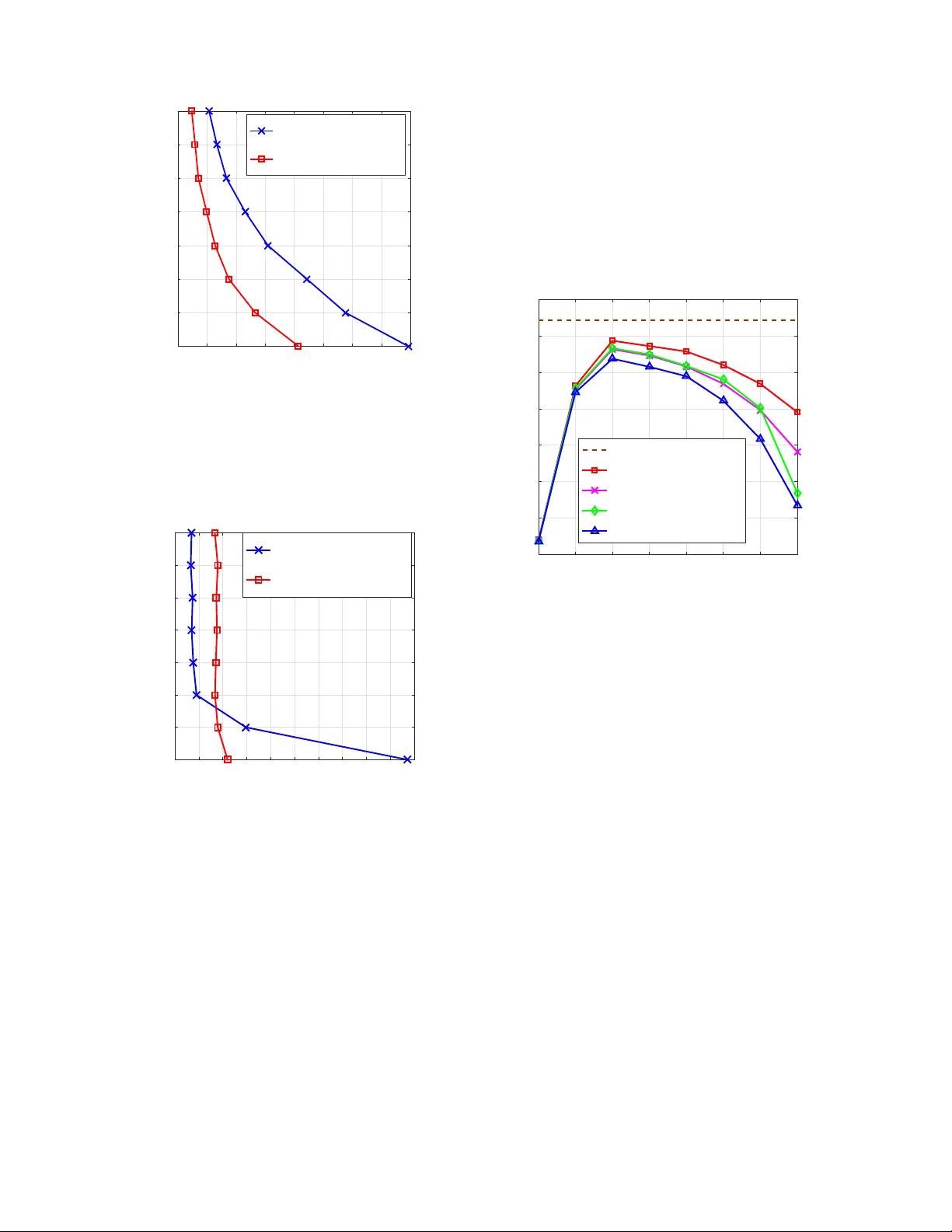
Decision Set Optimization and Ener gy-Ef ficient MIMO Communications Hang Zou ∗ , Chao Zhang ∗ , Samson Lasaulce ∗ , Lucas Saludjian † and Patrick P anciatici † ∗ LSS, CNRS-CentraleSupelec-Univ . Paris Sud, Gif-sur -Yvette, France Email: { hang.zou chao.zhang samson.lasaulce } @l2s.centralesupelec.fr † R TE, France Abstract —Assuming that the number of possible deci- sions for a transmitter (e.g ., the number of possible beam- forming vectors) has to be finite and is given, this paper in vestigates f or the first time the problem of determining the best decision set when energy-efficiency maximization is pursued. W e pr opose a framework to find a good (finite) decision set which induces a minimal performance loss w .r .t. to the continuous case. W e exploit this framework for a scenario of energy-efficient MIMO communications in which transmit power and beamforming vectors ha ve to be adapted jointly to the channel given under finite-rate feedback. T o determine a good decision set we propose an algorithm which combines the approach of In vasive W eed Optimization (IW O) and an Evolutionary Algorithm (EA). W e provide a numerical analysis which illustrates the benefits of our point of view . In particular , given a performance loss level, the feedback rate can by reduced by 2 when the transmit decision set has been designed properly by using our algorithm. The impact on energy- efficiency is also seen to be significant. Index T erms —Energy-Efficiency , Evolutionary Algo- rithms, Po wer Control, Quantization, Resource Allocation The literature of wireless communications comprises a large number of works on resource allocation problems at the transmitter side. The transmitter may hav e to choose e.g., its transmission power , its precoding matrix, or its modulation coding scheme (MCS). Almost always the corresponding decision set is taken for granted, as a data of the problem. In the present work, we show this might be questionable and that the choice of optimization set itself may be optimized. In fact, many practical reasons for operating with a finite decision set at the transmitter may be gi ven: computational complexity lim- itations at the transmitter , finite feedback-rate limitations, implementability requirements, robustness needs, stan- dardization requirements, etc. The motiv ation retained in this paper is the presence of a finite-rate feedback (FRF) mechanism. One of reasons for this is that the design of feedback mechanisms, protocols, or channels attracts a lot of attention of the community . The benefit from designing carefully the feedback system is of particular interest for 5G communications for which high data rates are pursued while managing very ef ficiently the av ailable energy resources. When inspecting the literature of feedback mecha- nisms, it is seen that some successful analog feedback mechanisms have been proposed (see e.g., [6], [7]) but more and more attention has been giv en to digital feedback techniques, a.k.a., limited-rate feedback (LRF) or FRF [3], [8]. Although the problem of resource allocation at the transmitter under FRF is quite well- known, the problem of designing the transmitter decision set under FRF has been left largely unexplored. The closest works to the one reported in this paper seem to be those concerning the maximization of capacity of MIMO communications. In particular, in [1] [3], the authors study the problem of designing the transmit codebook in presence of FRF . In [1], it is shown that the best beamforming vectors can be obtained ov er a Grassmannian manifold and the capacity loss induced by limited feedback can be upper bounded in a tight manner . In [3], a fundamental performance analysis is conducted to assess the loss in terms of sum-capacity of a MIMO broadcast channel in presence of FRF . A new Lloyd-Max-type algorithm is proposed by treating the beamforming vector selection problem as a vector quantization (VQ) problem for capacity maximization under FRF in [8]. The ergodic secrecy capacity of a wiretap channel is inv estigated under FRF in [9], as an application to secure communications. Although other works on the design of the codebook for capacity optimization might be cited, few papers (see [4]) hav e addressed the problem of designing a codebook for channel state information (CSI) feedback to hav e an energy-ef ficient MIMO communication. It appears that almost all papers of the authors’ knowledge assume a giv en set or space for the possible transmit vectors used to maximize energy-ef ficiency [14]. Motiv ated by this observation, one of the objectives of this paper is to propose a methodology to determine a good decision set which can be applied to maximize MIMO energy- efficienc y but also to maximize more general utility functions. The rest of the paper is organized as follows. The system model and the problem of finding a good de- cision set for energy-ef ficient MIMO communications is introduced in Sec. I. T o effecti vely determine the optimal decision set for this scenario, we propose in Sec. III an algorithm which combines the approach of In vasi ve W eed Optimization (IWO) and an e volutionary algorithm; this algorithm may be applied to more general utility functions. In Sec. IV, we provide a numerical perform analysis which strongly supports our frame work and shows the benefits e.g., in terms of feedback rate from designing the transmission decision set carefully . I . P R O B L E M F O R M U L A T I O N The considered communication scenario comprises a multi-antenna transmitter which has to adapt the transmit power p ∈ [0 , P max ] and its unit beamforming vector ω ∈ C N t × 1 ( k ω k = 1 ) to the realization of the channel transfer matrix H ∈ C N r × N t , N t and N r being respectiv ely the number of transmit antennas and receive antennas. W e assume that e very entry of H is circularly symmetric complex Gaussian distributed according to C N (0 , 1) . The action or decision of the transmitter is thus gi ven by the pair x = ( p, ω ) . The objectiv e of the transmitter is to maximize its energy-ef ficiency by adapting its decision to the channel. A very common measure of energy-ef ficiency is giv en by the ratio of a benefit function (e.g., the packet success rate or a measure of the transmission rate) to a cost po wer (e.g., an increasing function of the radiated power). The assumed utility function has the following form: u i ( x ; H ) : = V i ( x ; H ) C ( x ) (1) where V i ( x ; H ) is the transmission benefit obtained from choosing decision x over a channel matrix H and C ( x ) the transmission cost of using decision x ; i stands for the considered case index, the two cases being defined just next. Indeed, for the benefit function , we will use one of the following functions: • Case I benefit function (capacity function): V I ( p, ω ; H ) = log  1 + p k H ω k 2 σ 2  (see e.g., [17] [14]). • Case II benefit function (pac ket success rate) : V II ( p, ω ; H ) = R 0 exp  − cσ 2 p k H ω k 2  introduced in [17], where c > 0 is a constant related to the spectral efficiency of the system and R 0 the raw transmission rate. A well-admitted transmission cost function is as follo ws [19]: C ( x ) = C ( p, ω ) = p + P 0 (2) where P 0 represents a static cost such as the circuit power or the computation power . Giv en the fact that the utility consists of the ratio of a concav e function to an af fine function, it is well kno wn that the resulting utility in Cases I and II is a pseudo- concav e (PC) function [15]. Moreover , another common point between the two above functions is that the beam- forming vector only influences the energy-ef ficiency through the equiv alent channel gain g = k H ω k 2 and that the functions are monotonically increasing w .r .t. g for a fixed transmit po wer . In the presence of a FRF link to acquire the parameter g , which corresponds to the channel gain in our problem, the conv entional approach consists in quantizing the parameter g and then to report to the transmitter the quantized v alue of g through the feedback channel. Then, the transmitter maximizes the utility u based on the noisy value of g . Note that, with this approach, the decision set may be continuous. W ith the proposed approach described in Sec. III, the receiv er directly reports the decision index to the transmitter and the index rate is chosen to meet the feedback channel requirements such as the finite-rate feedback constraint. Let respecti vely denote by M 1 and M 2 the cardinali- ties of the power level set and the beamforming vector set. These sets are denoted by: P = { p 1 , . . . , p M 1 } and Ω = { ω 1 , . . . , ω M 2 } . W e define the required amount of feedback information to take a decision by B i = log 2 M i , which expresses in bit per decision. In 5G networks, one desirable scenario will be to be able to maximize energy-ef ficiency under some QoS constraints e.g., for URLLC [10], [11]. Obviously , the choice of the transmission decision set can have an impact on the QoS. This is the reason why we should introduce a transmission reliability constraint for the forward communication link (transmitter → receiv er) and a delay constraint for the rev erse of feedback com- munication link (receiv er → transmitter). If the data rate from the transmitter to the receiv er has to exceed the minimum rate r 0 , this induces a constraint on the benefit function V i . Equally , if the maximum delay to transfer the channel state information from the receiver to the transmitter is t 0 , the sum information-rate therefore has to meet the constraint B 1 + B 2 ≤ Rt 0 , R being the av ailable feedback channel rate. Having introduced these notations and made these observations, the decision set OP writes in the case of energy-efficient power control and beamforming as: max B 1 ,B 2 , P ,Ω E H " V i  b p ? P ( H ) , b ω ? Ω ( H ) ; H  b p ? P ( H ) + P 0 # s.t. − E H  V II  b p ? P ( H ) , b ω ? Ω ( H ) ; H  + r 0 ≤ 0 B 1 + B 2 − Rt 0 ≤ 0 (3) where b ω ? Ω ( H ) ∈ arg max ω ∈ Ω k H ω k 2 (4) and b p ? P ( H ) ∈ arg max p ∈P V i  p, b ω ? Ω ( H ) ; H  p + P 0 . (5) I I . A U X I L I A RY R E S U LT S The purpose of this section is twofold. First, we show how to simplify the OP under consideration and thus allow it to be solved more easily by the algorithm proposed in Sec. III. Second, we provide the solution of the OP in the limiting case where the number of decisions is infinite, which corresponds to the ideal situation where continuous decisions can be taken (based on perfect CSI feedback typically). A. Simplification of the original optimization problem Solving OP in (3) with usual numerical techniques may be difficult. The main reasons are as follows: 1) The OP in (3) is a mixed-inte ger OP . 2) W e are searching the optimal decision set instead of the optimal decision pair , which is more inv olv- ing computational speaking. 3) The quantities b ω ? Ω ( H ) and b p ? P ( H ) are defined in arg max -form which is difficult to ev aluate explicitly . Therefore, to circumvent the abov e difficulties we pro- pose to use sev eral ke y ingredients which allows one to still solve this non-tri vial problem. First, it can be noticed that at optimality all the budget of feedback information should be used that is, at optimality we hav e that B 1 + B 2 = Rt 0 . Second, we can split (3) into some sub-OPs OP ( B 1 , B 2 ) for ( B 1 , B 2 ) fixed. Third, in practice, Monte-Carlo simulations can be used to approximate the average utility . Indeed, assume a sequence of N channel realizations H = { H ` } N ` =1 has been generated, we then only need to solve OP ( B 1 , B 2 ) for ev ery possible configuration ( B 1 , B 2 ) . Denote ∆[ M ] the set of all subsets with cardinality M of a uni versal set, the optimal solution is obviously the configuration that yields the best performance among all sub-OPs OP ( B 1 , B 2 ) , ( P , Ω ) ∈ ∆[ M 1 ] × ∆[ M 2 ] , defined as: max ( P ,Ω ) 1 N N X ` =1 ( V i  b p ? P ( H ` ) , b ω ? Ω ( H ` ) ; H `  b p ? P ( H ` ) + P 0 ) s.t. 1 N N X ` =1  V II  b p ? P ( H ` ) , b ω ? Ω ( H ` ) ; H `  − r 0 ≥ 0 . (6) B. Solution for the limiting case of continuous decisions If the number of feedback bits B 1 and B 2 tend to infinity , obviously the OP defined in (3) boils down to a simple continuous OP . The optimal solution of the continuous OP for Utility functions I and II is giv en by the following proposition 1: Proposition 1. The pair of beamforming vector and power level maximizing the Case I and Case II utility function for channel r ealization H is given by: ( ω ? ( H ) = v ( H ) p ? i ( H ) = min { p i ( λ max ) , P max } (7) wher e v ( H ) is the dominant right vector correspond- ing to the larg est singular value of matrix H and λ max = k H v k 2 , p I ( λ max ) is the unique solution of the following equation: log  1 + λ max p σ 2  − p + P 0 p + σ 2 λ max = 0 (8) and p II ( λ max ) = cσ 2 2 λ max 1 + r 1 + 4 λ max P 0 cσ 2 ! (9) Pr oof: see Appendix A. It is worth mentioning that the optimal solution in continuous decision set is exactly the one corresponding to the situation where transmitter has perfect CSI (CSIT). I I I . P R O P O S E D A L G O R I T H M As already explained, to our knowledge, the problem of determining the optimal decision set has not been tackled in the related wireless literature and the one on energy-ef ficient communications in particular . Therefore, we had to determine a numerical technique to be able to effecti vely compute the optimal decision set. A natural way of doing so is to resort to learning. Unfortunately , there doesn’t seem to exist a ”plug-and-play” learning technique which is directly applicable to our problem. For instance, existing reinforcement learning techniques are not suited to find a decision set in a high dimensional continuous set under acceptable complexity . A Lloyd- Max-type algorithm could be used for solving OP in (6). Howe ver it is well kno wn that finding explicit regions for Lloyd-Max-type algorithm is time-consuming. There we propose here one possible way of solving the problem. More advanced techniques may be found or designed, constituting possible extensions of this paper . Here, our goal was to find a suitable candidate which proves the potential of our new approach over the con ventional approach (which consists in quantizing the parameter information such as the channel state information). IWO-DE algorithm is firstly proposed in [23] by combining IWO [21] and DE [22] which are essentially two evolutionary algorithms. Evolutionary algorithms hav e been widely used in many areas with its benefits such as simple computation, robustness and etc (see [18]). W e modified the IWO-DE algorithm to adapt our QoS constraint and our search space which is mainly the (2 N t − 1) -dimensional unit sphere. It appears that OP in (6) is e xtremely suitable to be solved by ev olutionary algorithms because the constraint acts as a selection action, i.e., all gener- ated solutions violate the constraint will be easily re- mov ed. W e modified the IWO-DE algorithm to inte- grate the QoS constraint and deal with our specific search space. T o giv e more focus on the importance of beamforming and for simplicity , we will assume a set of transmit power levels which are equally spaced: P = n 0 , 1 M 1 − 1 P max , 2 M 1 − 1 P max , . . . , M 1 − 1 M 1 − 1 P max o . The fitness function can be naturally constructed from (6): U i ( Ω ) : = 1 N N X ` =1 ( V i  b p ? P ( H ` ) , b ω ? Ω ( H ` ) ; H `  b p ? P ( H ` ) + P 0 ) . (10) T o make the computation tasks more conv enient, we introduce the matrix Ω = [ ω 1 , . . . , ω M 2 ] , which is constructed from the set Ω = { ω 1 , . . . , ω M 2 } . The algorithm we propose comprises the following steps: • Initialization: randomly choose W beamforming sets in the search space: Ω (0) 1 , . . . , Ω (0) W as the primitiv e population. W is called the population size. Ω ( t ) k denotes the k -th indi vidual of the t -th generation. • Reproduction : every individual reproduces its off- spring according to their fitness. The number of offspring for k -th individual at ( t + 1) -th generation S ( t +1) k is giv en by: S ( t +1) k = υ  Ω ( t ) k  [ S M − S m ] + S m (11) where υ  Ω ( t ) k  = U  Ω ( t ) k  − min i U  Ω ( t ) i  max i U  Ω ( t ) i  − min i U  Ω ( t ) i  , (12) S M and S m are respectiv ely the maximum and minimum numbers of offspring that an individual is allowed to reproduce. • Spatial Dispersion: for k -th indi vidual, its off- spring obeys a complex Gaussian distribution O ( t ) k ∼ N  Ω ( t ) k , µ ( t ) + µ ( t ) i  . Then ev ery column vector being essentially a beamforming vector will be normalized. In what follows, a normalization procedure will be performed once there is a pos- sibility that new produced beamforming vector di- ver ges from the unit sphere. Every individual repro- duces its offspring in the feasible set till it achieves the number giv en by (11). µ ( t ) is the standard deriv ation for ev ery entry of Ω ( t ) k controlling the div ergence of the dispersion. The ev olution of µ ( t ) through the generations is giv en by: µ ( t ) =  T − t T  γ  µ ini − µ end  + µ end (13) where γ is called the nonlinear index and µ ini and µ end stands for the initial and final standard deriv ation, respectiv ely . In general, we should hav e µ ini  µ end in order to av oid dropping into a local maximum and µ end → 0 to increase the accuracy near the potential global optimum. • Competitive Exclusion: sort all the of fspring to- gether with their parental indi viduals in ascending order according to their fitness. Then select the W first offspring as the original material for next generation: Φ ( t ) 1 , . . . , Φ ( t ) W s.t. U  Φ ( t ) 1  ≥ · · · ≥ U  Φ ( t ) k  ≥ U  Φ ( t ) W  . • Mutation: there are many dif ferent strategies for creating mutations. For example, for the k -th po- tential individual, we create its possible mutant by: Ψ ( t ) k = Ψ ( t ) idx 1 + F 0  Ψ ( t ) idx 2 − Ψ ( t ) idx 3  , where F 0 is called the scaling factor . And we further choose idx 1 = 1 (the best one), idx 2 = r and (2 , W ) and idx 3 = rand (2 , W ) with idx 2 6 = idx 3 and idx 2 , idx 3 6 = k . • Crossov er: for the l -th component of the k -th individual at next generation ω ( t +1) k,l , we let ω ( t +1) k,l = ( ψ ( t ) k,l , y l ≤ C r or l = L r φ ( t ) k,l , otherwise where ω ( t +1) k,l , ψ ( t ) k,l and φ ( t ) k,l is the l -th component of Ω ( t +1) k , Ψ ( t ) k and Φ ( t ) k , respectiv ely , y l is a random variable uniformly distributed ov er [0 , 1] , C r is called the crossover probability and L r is a randomly chosen index so that the mutant decision set can’t be identical to the original one. • Selection Operation: only mutant decision in- creases the fitness ( U  Ω ( t +1) k  > U  Φ ( t ) k  ) will be conserved. Otherwise, Ω ( t +1) k = Φ ( t ) k . If the initial population is well selected, the population of beamforming sets will conv erge to the optimal direction set Ω ? for a sufficiently large number of generations. I V . N U M E R I C A L R E S U LT S One of the main objectiv es of this section is to show that the proposed approach may bring some significant improv ements when compared to the conv entional ap- proach. The con ventional approach consists in quantizing the channel state and reporting the corresponding infor- mation to the transmitter . In most real systems and exist- ing standards, uniform quantization is implemented. The av erage av ailable amount of feedback information is thus B 2 N t per channel use. Here, we consider a more advanced quantizer namely , the Lloyd-Max (LM) quantizer in [24]. Essentially , the LM quantizer consists in determining the quantization cells and representativ es in an iterativ e manner to minimize the distortion E  k g − b g k 2  , b g being the quantized channel. This quantized information is then used by the transmitter to maximize its utility function u i ( x ; g ) . W e will refer to this algorithm as the “best con ventional appr oach in SO T A” . Moreov er , the random vector quantization (R VQ) scheme should be taken as reference as well which is proved to be near-optimal for moderate information feedback of capacity maximization problem in [2]. For the simulation setting, we will consider a typical scenario defined by: N t = 4 ; N r = 1 ; r 0 = 3 × 10 5 bps , t 0 = 0 . 01 s ; R 0 = 10 6 bps ; c = 0 . 1 ; P 0 = 0 . 5 mW ; P max = 1 mW ; σ 2 = 1 mW . Similarly , for the the IWO-DE algorithm, a typical setting (in coherence with related evolutionary algorithms) will be assumed as in T able I. T ABLE I P A R A M ET E R S E T TI N G F O R I W O- D E Parameters V alue Population size W 10 number of generations T 400 max number of offspring S M 20 min number of offspring S m 10 Non-linear index γ 2.5 Initial standard deriv ation µ ini 1 N t Final standard deriv ation µ end 1 200 N t Scaling factor F 0 0.9 Crossover probability C r 0.9 In order to clarify the impact of the po wer and beam- forming separately , we consider two following different situations: 1) When the influence of B i is assessed, B j ( j 6 = i ) is fixed. 2) W e fix the total number of quantization bits B = B 1 + B 2 . W e introduce a key quantity which is the Relative Optimality Loss: σ (%) = U CSIT − U FRF U CSIT × 100% (14) where U CSIT is the maximum utility achiev ed by the transmitter when the perfect knowledge of CSI g is av ailable at the transmitter and U FRF is the maximum utility achieved by the transmitter in presence of fi- nite rate feedback (FRF). The latter may assume the con ventional approach (relying on the LM quantizer or uniform quantizer) , the proposed approach (relying on the decision set optimization) and R VQ. A. Separate quantization over beamforming or power levels First of all, we fix B 1 = 4 bits and analyze the influence of B 2 to the relativ e optimality loss. T o compare our approach with the con ventional approach, Fig. 1 illustrates the required amount of information for beamforming quantization to achiev e a giv en relativ e optimality loss of case I utility function. F or a gi ven same optimality loss, remarkably , one can observe that with our approach one can reduce by a factor 2 the amount of beamforming bits with respect to the LM quantizer and R VQ. In addition, if the number of bits allocated to beamforming quantization is quite small, the relati ve optimality loss remains acceptable for the proposed approach while it is large for other existing solutions. Moreov er , to explore the impact of utility function on beamforming quantization. Fig. 2 compares the required B 2 to achiev e a given optimality loss between the utility Relative Optimality Loss (%) 0 5 10 15 20 25 30 35 40 45 Required amout of info (bits/decision) 1 2 3 4 5 6 7 8 Uniform quantizer RVQ in [4] Llyod-Max quantizer Proposed algorithm Fig. 1. The benefits from using our algorithm is very apparent on this figure. For example, for an optimality loss of 5% between the perfect CSI case and the finite-rate feedback case, the amount of information needed to perform beamforming can be reduced by around 2 by moving from the best state-of-the-art approach to the proposed approach. Here, Case II and B 1 = 4 bits/decision are assumed. functions in case I and the utility function in case II. By implementing the proposed quantization scheme, the minimum number of bits for EE of case II is larger than the EE of case I for achieving the same performance which may suggests that the EE of case II (packet transmission success rate) is slightly sensitiv e to the quality of quantization than EE of case I (capacity) and thus worth more feedback bits and better beamforming code book design techniques. T o see the influence of the po wer level quantization, we fix the bits of beamforming quantization as B 2 = 6 and vary the bits for power level feedback from 1 to 8 . Fig. 3 shows the ev olution of required amount of information for po wer quantization as function of relati ve optimality loss. For EE of case I , dif ferent from EE of case II, increasing the number of bits for power quantization have less important impact on performance of the system. This improv ement is always modest while the improvement is firstly sharp when few bits are av ailable but then becomes modest with enough number of bits provided for EE of case II. Thus if the bits for beamforming quantization are sufficient ev en one bit feedback information about power provides acceptable performance for EE of case I. Up to now , W e can conclude that EE of case II is sensiti ve to both the quality of beamforming quantization and power quantization combing the observation in Fig. 1 and Fig. 2. W e need to further find the optimal bits allocation policy for EE of case II in Section IV -B. Relative Optimality Loss (%) 0 5 10 15 20 25 30 35 40 Required amount of info (bits/decision) 1 2 3 4 5 6 7 8 Case II utility function Case I utility function Fig. 2. Here, the influence of the utility function on the obtained results is assessed. It is clearly seen that some utilities require more feedback than others. Here, it is seen that considering the pack et success rate for the benefit function (Case II) requires more feedback resources than using the capacity function (Case I). Remarkably , it is possible to quantify this extra amount of resources. Here, it is assumed that B 1 = 4 bits/decision. Relative Optimality Loss (%) 0 5 10 15 20 25 30 35 40 45 50 Required amount of info (bits/decision) 1 2 3 4 5 6 7 8 Case II utility function Case I utility function Fig. 3. The impact of B 2 on the preceding observ ation is assessed. Here, with B 2 = 6 bits/decision, the curves are much steeper , indicating that the choice of the number of feedback rate is more critical in this regime as soon as small optimality losses are desired. B. Joint Quantization According to the precedent observations, finding a proper allocation polic y between B 1 and B 2 is necessary . In order to determine the optimal allocation of bits for EE of case II , we assume that the total quantization bits are fix ed so that the transmitter merely seeds the essential information back to the receiv er . W e fix the total number of bits for quantization as B = 8 (e xactly one byte). Fig. 4 sho ws the ev olution of energy efficiency of case II as function of quantization bits used for beamforming. T o achiev e the best performance, among 8 total quantization bits, we should allocate 3 bits for beamforming quan- tization and 5 bits for power quantization. Moreover , for all methods, sufficient number of bits should be conserved to beamforming quantization by observing the sharp decay of av erage utility for 1 ≤ B 2 ≤ 3 . Finally , ev en no information provided for po wer le vel ( B 2 = 8 ), the energy efficiency achie ved by our proposed approach and R VQ is acceptable which shows the importance of quantizing directly on the decision itself instead of quantizing the CSI in the con ventional approach. Required amount of info (bits/decision) 1 2 3 4 5 6 7 8 Energy Efficiency (Mbps/J) 0.6 0.7 0.8 0.9 1 1.1 1.2 1.3 Perfect CSIT Proposed algorithm RVQ in [4] Llyod-Max quantizer Uniform quantizer Fig. 4. Here, the gain brought by our approach are measured in terms of EE for case II. The con ventional approach is sensitiv e to the available amount of feedback information for beamforming when power level quantization is rough while the proposed approach offers good performance for a large range of feedback rates. V . C O N C L U S I O N S This paper treats for the first time the problem of finding jointly set of power lev el and beamforming vectors for energy-ef ficient communications. While the problem is relativ ely easy to solve when decisions can be continuous, the problem needs to be formulated properly when the decision set is imposed to be finite. W e pre- cisely propose this new formulation of the problem. The problem of determining an optimal decision set appears. Whereas the latter problem may be difficult in general, we show that it can be solved for the wireless application of interest. For this, we propose a new algorithm, which is referred to the IWO-DE algorithm. It allows us to search for optimal sets of beamforming vectors over the ( 2 N t − 1 )-dimensional unit sphere. When applied to energy-ef ficient communications, our approach is shown to outperform the best state-of-the-art techniques such as Lloyd-Max algorithm and R VQ. Ob viously , our approach needs to be explored and developed further . In particular , when the system dimensions increase, complexity issues need to be considered. When there is interference, the proposed framework needs to be extended. In the pres- ence of interactions between the decision-makers, other issues such as Braess paradoxes may arise and make the problem ev en more challenging. A C K N O W L E D G M E N T This work has been funded by the R TE- CentraleSupelec Chair on “The Digital Transformation of Electricity Networks”. A P P E N D I X A For a fixed power p , maximizing the utility I is equiv alent to maximize the equiv alent channel gain g = k H w k 2 . Thus the optimal beamforming v ector is giv en by the right dominant vector v which is the right vector corresponding to the largest singular value √ λ max of H . Thus the maximum of equi valent channel gain is giv en by G max = k H v k 2 = λ max , then ∂ u ∂ p = − ln  1 + λ max p σ 2  + p + P 0 p + σ 2 λ max ( p + P 0 ) 2 Define f ( p ) = − ln  1 + λ max p σ 2  + p + P 0 p + σ 2 λ max , one has: f 0 ( p ) = − 1 p + σ 2 λ max − σ 2 λ max − P 0  p + σ 2 λ max  2 • If σ 2 λ max ≥ P 0 then f 0 ( p ) < 0 for ∀ p > 0 mean- ing f ( p ) is a monotonically decreasing function. Furthermore, we hav e f (0) = λ max P 0 σ 2 > 0 and f (+ ∞ ) = −∞ < 0 , there exists an unique solution p I ( λ max ) of the Eq. 9 by mean-value theorem. • If σ 2 λ max < P 0 then f 0 ( p ) > 0 for 0 < p < P 0 − σ 2 λ max and f 0 ( p ) > 0 for 0 < p < P 0 − σ 2 λ max . There- fore max f ( p ) = f  P 0 − σ 2 λ max  > f (0) > 0 . W ith the same argument, there exists an unique so- lution p I ( λ max ) of the Eq. 9 in  P 0 − σ 2 λ max , + ∞  . Moreov er we have f ( p ) > 0 for 0 < p < p I ( λ max ) and f ( p ) < 0 for p > p I ( λ max ) . Finally the optimal po wer p ? ( H ) for channel realization H is giv en by: p ? ( H ) = min { p I ( λ max ) , P max } The proof for Case II utility function can be obtained by using similar arguments abo ve. R E F E R E N C E S [1] D. Love, R. Heath, and T . Strohmer, “Grassmannian beamform- ing for multiple-input multiple-output wireless system”, IEEE T rans. Inform. Theory , vol. 49, no. 10, pp. 2735-2747, Oct. 2003. [2] C. K. Au-yeung and D. Love , “On the performance of random vector quantization limited feedback beamforming in a MISO system”, IEEE T rans. on Signal Processing , vol. 6, pp. 458-462, Feb . 2007. [3] N. Jindal, “MIMO Broadcast Channels With Finite-Rate Feed- back, T rans. Inform. Theory , vol. 52, no. 11, Nov . 2006. [4] O. Amin, E. Bedeer , M. H. Ahmed and O. A. Dobre, “ A Novel Energy Efficient Scheme With a Finite-Rate Feedback Channel”, IEEE Communications Letters , VOL. 3, NO. 5, October 2014. [5] H. Zou, C. Zhang, S. Lasaulce, L. Saludjian and P . Panciatici, “Decision-Oriented Communications: Application to Energy- Efficient Resource Allocation”, In pr oceedings of WINCOM 2018 (in vited paper), Marrakesh, Morocco. [6] G. Caire, N. Jindal and M. Kobayashi, “ Achie vable rates of MIMO downlink beamforming with non-perfect CSI: a com- parison between quantized and analog feedback”, 2006 F ortieth Asilomar Conference on Signals, Systems and Computers , Pacific Grove, CA, USA. [7] T .L. Marzetta, B.M. Hochwald, “Fast Transfer of Channel State Information in Wireless Systems”, IEEE T ransactions on Signal Pr ocessing , VOL. 54, June 2004. [8] J.C. Roh, B.D. Rao, “Transmit Beamforming in Multiple- Antenna Systems With Finite Rate Feedback: A VQ-Based Approach”, IEEE T rans. Inf. Theory , VOL. 52, NO.3, 2006. [9] A. Hyadi, Z. Rezki and M. Alouini, “Secure Multiple-Antenna Block-Fading W iretap Channels W ith Limited CSI Feedback”, IEEE T rans. on Wir eless Commun. , VOL. 16, NO. 20, 2017. [10] X. He, H. Xing, Y . Chen and A. Nallanathan, “Energy-Efficient Mobile-Edge Computation Offloading for Applications with Shared Data”, In pr oceedings of Globecom 2018 , Abu Dhabi, U AE. [11] Y . W ang, M. Zhou, Z. T ian and W . T an y , “Beamforming and Artificial Noise Design for Energy Efficient Cloud RAN with CSI Uncertainty”, In proceedings of Globecom 2018 , Abu Dhabi, U AE. [12] R. Radner, “T eam decision problems”, The Annals of Mathemat- ical Statistics , 33(3):857-881, 1962. [13] S. Liu, L. Xie and D.E. Que vedo, “Event-Triggered Quantized Communication-Based Distributed Con vex Optimization”, IEEE T rans. on Contr . of Network Systems , VOL. 5, NO. 1, 2018. [14] A. Zappone, E. Bj ¨ ornson, L. Sanguinetti and E. Jorswieck, “Globally optimal energy-ef ficient power control and receiver design in wireless networks”, IEEE T rans. on Signal Pr ocessing , 2017. [15] A. Zappone and E. Jorswieck, “Energy efficienc y in wireless networks via fractional programming theory”, F oundations and T r ends in Communications and Information Theory , V OL. 11, NO. 3-4, 2015. [16] A. Zappone, Z. Chong and E. Jorswieck, “Energy-A ware Com- petitiv e Power Control in Relay-Assisted Interference W ire- less Networks”, IEEE Tr ansactions on W ir eless Communication , vol.12, 2013. [17] E. V . Belmega and S. Lasaulce, “Energy-Efficient Precoding for Multiple-Antenna T erminals” IEEE T ransactions on Signal Pr ocessing , vol. 59, no. 1, January 2011. [18] David B. Fogel, “The Advantages of Evolutionary Computation”, In Pr oceeding of Biocomputing and emer gent computation , page 1-11, 1997. [19] F . Richter , A. J. Fehske, and G. Fettweis, “Energy Efficiency Aspects of Base Station Deployment Strategies for Cellular Networks, IEEE Proceedings of VTC , Fall’2009. [20] K. Arulkumaran, M.P . Deisenroth, M. Brundage and A.A. Bharath, “Deep Reinforcement Learning: A brief Survey”, Deep Learning for V isual Understanding , 13 november 2017. [21] A. Mehrabian and C. Lucas, “ A novel numerical optimization algorithm inspired from weed colonization”, Ecol. Inform. , vol. 1, no. 4, pp. 355366, Dec. 2006. [22] R. Storn and K. Price, “Differential Evolution: A Simple and Efficient Heuristic for Global Optimization over Continuous Spaces”, Journal of Global Optimization , 11: 341-359, 1997. [23] X. Cai, Z. Hu, and Z. Fan, “ A novel memetic algorithm based on in vasi ve weed optimization and differential ev olution for constrained optimization, Soft Computing , vol. 17, no. 10, pp. 1893-1910, Oct. 2013. [24] S. Lloyd, “Least squares quantization in PCM”, IEEE Tr ansac- tions on Information Theory , 28(2), 129-137, 1982.